Ch 3 Python Example Code¶

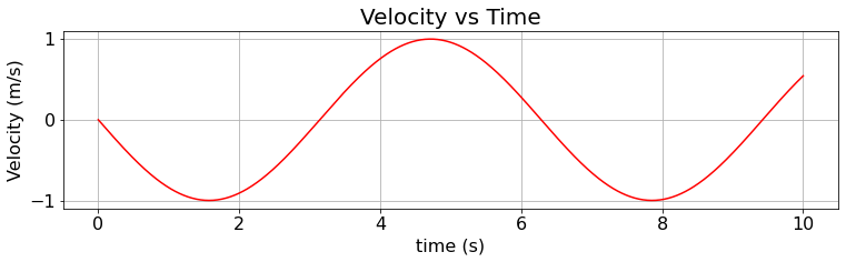
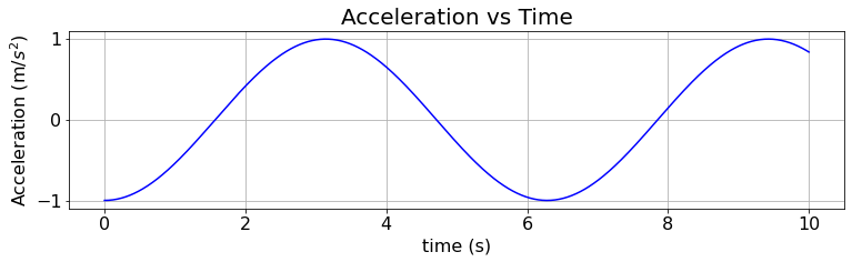
Example Code for use with additional problems added to Chapter 3, specifically plots for Simple Harmonic Motion for displacement, velocity, and acceleration.

We will assume a phase shift of zero for all exercises and start with a basic solution equation of $x = x_0\cos{\omega_0t}$ .

import matplotlib.pyplot as plt              # for ease of use
import numpy as np                           # for the needed math functions

plt.rcParams['figure.figsize'] = 12.5,10     # default plot size

# the example code is for a basic spring-mass system
# the spring is ideal and the surface is frictionless

# define the basic constants of the system
x0 = 1     # amplitude or initial displacement
k = 1      # spring constant
m = 1      # mass of the block
Omega0 = (k / m)**(0.5)

# Define Displacement function
def Displacement(t):
    return x0 * np.cos(Omega0 * t)

# define the Velocity function
def Velocity(t):
    return -Omega0 * x0 * np.sin(Omega0 * t)

# define the Acceleration function
def Acceleration(t):
    return -Omega0**2 * x0 * np.cos(Omega0 * t)

t = np.linspace(0, 10, 1000)                     # define t for smooth curve

# Display as three separate plots

plt.figure()                                    # set up the plot

plt.rcParams.update({'font.size': 16})

plt.subplot(3, 1, 1) # Displacement first
plt.plot(t, Displacement(t), color = "g")
plt.title("Displacement vs Time", fontsize = 20)
plt.xlabel("time (s)", fontsize = 16)
plt.ylabel("Displacement (m)", fontsize = 16)
plt.grid()
plt.show()

plt.subplot(3, 1, 2) # Velocity second
plt.plot(t, Velocity(t), color = "r")
plt.title("Velocity vs Time", fontsize = 20)
plt.xlabel("time (s)", fontsize = 16)
plt.ylabel("Velocity (m/s)", fontsize = 16)
plt.grid()
plt.show()

plt.subplot(3, 1, 3) # Acceleration third
plt.plot(t, Acceleration(t), color = "b")
plt.title("Acceleration vs Time", fontsize = 20)
plt.xlabel("time (s)", fontsize = 16)
plt.ylabel("Acceleration (m/$s^2$)", fontsize = 16)
plt.grid()
plt.show()

plt.subplots_adjust(left=0.1, bottom=0.1, right=0.9,
                    top=0.9, wspace=0.4, hspace=0.4)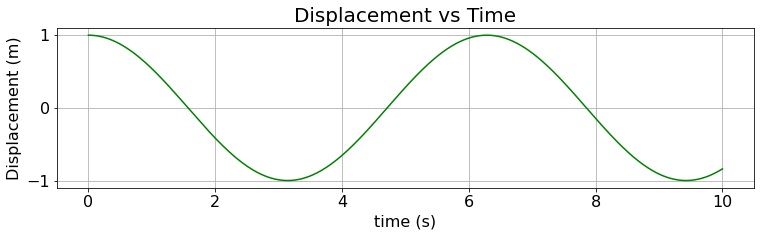

<Figure size 900x720 with 0 Axes>

# Expansion Question
# simple modifications to the example code

# A mass sits on a frictionless surface with a spring
# attached to each side as in the diagram. The springs
# have spring constants of $k_1$ and 3$k_1$ respectively.
# Find the differential equation of motion,
# and plot the equations for displacement,
# velocity, and acceleration.


# basic constants of the system can be set as desired
x0 = 1     # amplitude or initial displacement
k = 1      # spring constant
m = 1      # mass of the block

# Expansion question.

# A physical pendulum consisting of a simple rod of uniform
# density swinging from one end has an angular frequency of
# sqrt(3g/L). Assume you would like to create a number of
# versions of this pendulum for various uses, all with the
# same mass (of 1 kg) but having different lengths. Find
# the period for lengths between 10 cm and 1m and plot the
# results.

# Expansion question

# Refer to the pendulum-spring system of Sample
# Problem 3-2. Given its angular frequency of:
# sqrt((k \ m) + (g \ L)), find the equations for 
# displacement, velocity and acceleration.
# Plot these equations.