2. Newtonian Motion - Second-Year Dynamics

In this chapter, we will look at the universal laws of motion with emphasis on review of Newton’s Laws (mainly the second law) and free-body diagrams.

2.1 Universality of the Laws of Motion:¶

Classical mechanics describes how objects move. While this chapter is called Newtonian Motion after Sir Isaac Newton, it is important to recognize that Newton was not the first person to develop theories about the motion of objects. Physics is universal. Historically, physicists from all over the world also sought laws of motion hundreds to thousands of years before Newton.

2.2 Newton’s Three Laws of Motion:¶

Newton’s three laws of motion are a mathematical description connecting motion to forces. These laws apply to all objects of any size (above the atomic level), any shape, and any internal structure (solid or even liquid). The three laws are:

The law of inertia: A body moves with constant velocity unless acted on by a force.
The equation of motion: The change of momentum of a body equals the net force acting on it.
The law of action and reaction: For every force acting on a body, there is an equal and opposite reactive force.

The first law corresponds to the conservation of momentum. The idea here, is that an object with no forces acting on it will be at rest or moving at a constant velocity. It is important to note that the first law requires that you define an appropriate inertial frame (a frame of reference). Your inertial frame can be static (at rest) or in motion (with constant velocity, no acceleration). If your reference frame is accelerating, we call that a non-inertial frame and the physics is a bit different. We will discuss non-inertial frames in Chapters 4 and 5.

The second law corresponds to the rate of change of momentum, $\vec{p}$ . The net force acting on a system is:

\sum \vec{F} = \frac{\mathrm{d}\vec{p}}{\mathrm{d}t}

(1)

where the momentum is $\vec{p} = m\vec{v}$ . If your system has constant mass, then the second law can be written as:

\sum \vec{F} = m\vec{a} = m\ddot{\vec{r}}

(2)

See Chapter 1 for a review of vector notation.

The second law connects kinematics (changes in momentum or the acceleration of an object) to a dynamical force. In the case of a constant mass, Equation (2.1) has the more familiar form of Equation (2.2). However, there can be physics problems where the mass of the system is also allowed to change (e.g., if you are in a rocket that is using fuel). In these cases, you cannot use the more familiar $\vec{F} = m\vec{a}$ equation. We will discuss variable mass problems in Chapter 6.

Finally, the third law says that forces come in pairs. For two objects that are exerting forces on each other, those forces will be equal in magnitude and opposite in sign. That is,

\vec{F}_{12}= -\vec{F}_{21}

(3)

For example, when you stand on the ground, you push downward on the surface due to gravity. But you don’t fall into the surface, because the ground pushes back up on you in an equal and opposite force, typically called the normal force.

2.3 Static Systems¶

Static systems are systems that are not in motion. In this case, the sum of all forces $(\sum \vec{F}$ ) and the sum of all momenta $(\sum \vec{p}$ ) are both zero. Let’s look at a problem for a static system.

Sample Problem 2-1

Figure 2.1 shows two masses connected to each other by an ideal pulley. If this system is at rest, what is the magnitude of the force of friction?

Figure 2.1:Two masses are attached to an ideal string that runs along ideal pulley at the edge of an incline of angle $\theta$ . One mass sits on the incline and the other hangs off the edge of the incline. The incline has a coefficient of friction, $\mu$ . The system is at rest.

Solution

First, we find all the forces acting on the system. Since there are two masses, they will each have gravity $M_{1}g$ and $M_{2}g. M_{1}$ is sitting on the incline, so it is pushing down on the incline due to gravity and the incline is pushing up on $M_{1}$ via the normal force $N$ . Since $M_{2}$ is hanging, it does not have a normal force. Both masses are attached by a string so that means there is a tension $T$ for both. Since the string and pulley are ideal, they have no mass or friction. But there is a coefficient of friction acting on $M_{1}$ from the incline and the friction force is $f = \mu N$ , where $N$ is the normal force.

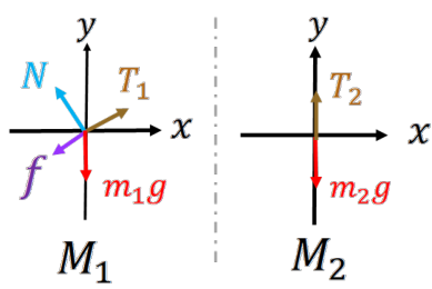
With the forces, let’s draw the free-body diagram. For simplicity, we’ll split up $M_{1}$ and $M_{2}$ into two different panels. The left panel in Figure 2.2 shows the free-body diagram for $M_{1}$ on the incline and the right panel is the free-body diagram for $M_{2}$ .

Figure shows free body diagrams for the two masses with standard 2D Cartesian axes. — Figure 2.2:Free-body diagram showing gravity $(mg)$ , tension $(T)$ , friction $(f)$ , and the normal force $(N)$ associated with Figure 2.1. Left panel is for $M_{1}$ , right panel is for $M_{2}$ .

Figure 2.2 shows the directions for all the forces, where gravity points down, the normal force is perpendicular to the incline, tension is along the string, and friction is parallel to the surface. Note that we need to assume a direction for friction. The actual direction of friction will depend on the relative masses for $M_{1}$ and $M_{2}$ (we do not know if $M_{1}$ wants to slide up or down the incline at this time). So we will make a guess for the direction of friction for now. If we guessed wrong, we will just get a negative force.

To find the net force on the system, we sum all forces for both masses. Since the string is ideal, it does not stretch or deform, which means that the tension on both sides of the pulley must be the same and $T_{1}= T_{2}$ .

For $M_{2}$ , there are only two forces, $T_{2}$ and $M_{2}g$ . Since both masses are at rest, the sum of all forces on $M_{2}$ must equal zero (Second Law). So we get $T_{2}= M_{2}g$ .

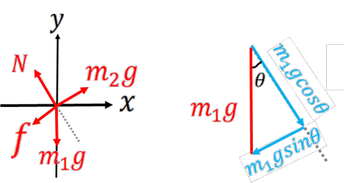
Combining $T_{1}= T_{2}$ and $T_{2}= M_{2}g$ , we can revisit the free-body diagram of $M_{1}$ . Figure 2.3 is an updated free-body diagram of $M_{1}$ only.

Figure 2.3 from the source textbook — Figure 2.3:Left: Free-body diagram of $M_{1}$ with $T_{1}= T_{2}= M_{2}g$ . Right: Vector diagram for the gravitational force on $M_{1}$ .

Continued

With Figure 2.3, we can solve for the normal force $N$ and friction $f$ . We break up the gravitational force into the component that is parallel to the incline and perpendicular to the incline. We can get these from trigonometry (see the right panel of Figure 2.3):

F_{g,//}= -M_{1}g\sin \theta

(4)

F_{g,\perp}= -M_{1}g\cos \theta

(5)

Note that we have defined up the incline and outward from the incline as positive.

For the system to be at rest, the sum of all forces must be zero. Since the components parallel to the incline $(f,F_{g,//},T_{1})$ are orthogonal to the components perpendicular to the incline $(N,F_{g,\perp})$ , they must each add to zero. That is, the sum of all parallel components must be zero and the sum of all perpendicular components must be zero. The two groups of forces act independently. Adding the individual forces in each group:

\begin{aligned} 0 &= \sum F_{\perp} \\ 0 &= \sum F_{//} \end{aligned}

(6)

\begin{aligned} 0 &= N - M_{1}g\cos \theta \\ 0 &= M_{2}g - M_{1}g\sin \theta - f \end{aligned}

(7)

\begin{aligned} N &= M_{1}g\cos \theta \\ f &= M_{2}g - M_{1}g\sin \theta \end{aligned}

(8)

Thus, we have our magnitude of $f$ . The true direction of $f$ will depend on $\theta, M_{1}$ , and $M_{2}$ . If $M_{2}g > M_{1}g\sin \theta$ , then $f$ is positive and our assumed direction for $f$ is correct. If $M_{2}g < M_{1}g\sin \theta$ , then $f$ will be negative, indicating that our assumed direction for $f$ was wrong. This case means that $M_{1}$ is so heavy that it will pull on $M_{2}$ (e.g., $M_{1}$ wants to move down the incline so friction is acting up the incline) .

If $M_{2}$ and $\theta$ are held constant, what is the maximum mass for $M_{1}$ before our assumed direction of friction from Figure 2.2 is wrong?
Recall that friction is defined by $f = \mu N$ , where $\mu$ is the coefficient of friction. If $M_{1}= M_{2}$ and the angle is $30^{\circ}$ , what is the value of $\mu$ ?

Figure 2.1 shows an ideal pulley system. When you have an ideal pulley system, it means that the pulley and rope extending over the pulley each have no mass and there is no friction between them. It also means that the rope will not deform (e.g., stretch) due to tension. So you can assume that the tension is the same everywhere in the rope.

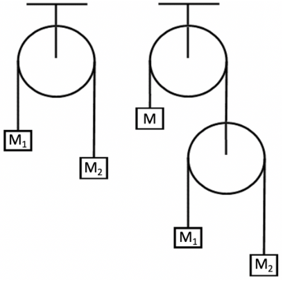
An Atwood machine is an ideal pulley system with masses attached by an ideal rope that hang from an ideal pulley. Figure 2.4 shows an example single Atwood machine (left image) and a double Atwood machine (right image). For the single Atwood machine, a single rope holds two masses, $M_{1}$ and $M_{2}$ , over an ideal pulley. The double Atwood machine has two ideal ropes: one connecting $M_{1}$ and $M_{2}$ and a second connecting $M$ to the lower pulley.

Figure shows simple examples of the single Atwood and double Atwood machines. — Figure 2.4:A single Atwood (left) and double Atwood (right) machine. The ropes and pulleys in each machine are ideal. The single Atwood machine has one rope (connecting $M_{1}$ and $M_{2})$ , whereas the double Atwood machine has lower rope connecting $M_{1}$ and $M_{2}$ and an upper rope connecting $M$ and the lower pulley.

Since ideal pulleys have no mass, they will have no net force acting on them (Newton’s second law). That condition makes them useful when equating forces to solve problems. Consider the free-body diagrams for the mass and pulley systems above. Whichever forces act on the pulleys will have to balance to zero.

2.4 Systems with Constant Acceleration¶

The simplest case for Newton’s laws is a system with constant acceleration and constant mass such that the net force is also constant $(\sum \vec{F} = m\vec{a}$ = constant).

Sample Problem 2-2

A person of height $r_{0}$ throws a ball at an angle of $\theta$ upwards from the ground with an initial speed of $v_{0}$ . What is the maximum height that the ball reaches? How far does the ball travel horizontally when it hits the ground?

Figure 2.5:Sketch of the ball’s trajectory. The ball starts at point A, rises up to a maximum at point B, and then hits the ground at point C a distance $x_{C}$ from the original starting point.

Solution

We will assume that the ball stays close to the ground such that we can approximate gravity as a constant force (we revisit gravity as a non-constant force in Chapter 10).

First, consider how the ball will move. Since the ball is given both a vertical and horizontal initial motion, this is a 2D problem. But the only source of acceleration is from gravity, which is constant and points downwards (gravity does not affect the horizontal motion).

Therefore, the ball will make an arc, with its vertical motion changing (due to the acceleration with gravity) and its horizontal motion held constant (we will ignore any air resistance). The motion along $x$ and $y$ are independent, so we can solve this problem by looking at each component separately.

What is the maximum height? This is point B in Figure 2.5. The maximum height depends only on the motion along the $y-$ axis, so we can ignore motion on the $x-$ axis. For the $y-$ axis motion, we have an acceleration of $a = -g$ , defining up as positive. Since $a = \frac{\mathrm{d}v}{\mathrm{d}t}$ , we can integrate to get the equation for velocity as a function of time. See also, Chapter 1 for more details.

$v_{y}= \int a$ d $t =\Rightarrow v_{y}$ is given by the integral of $a$ , which is a constant $v_{y}= -gt + C =\Rightarrow a = -g, C$ is the initial velocity along the $y-$ axis $v_{y}= -gt + v_{0}\sin \theta =\Rightarrow v_{0}\sin \theta$ is the initial velocity (see Figure 2.5)

For height, $y = \int v_{y}$ d $t$ . Integrating the velocity equation gives,

y = r_{0}+ v_{0}\sin \theta t - \frac{1}{2} gt^{2}=\Rightarrow r_{0}\mathrm{is} \mathrm{the} \mathrm{initial} \mathrm{height} \mathrm{of} \mathrm{the} \mathrm{ball}

(9)

To find the maximum height, $y_{B}$ , we need the time when the ball reaches the peak of motion, $t_{B}$ . At the peak, the vertical component of the velocity will be instantaneously zero.

0 = $-gt_{B}+ v_{0}\sin \theta =\Rightarrow$ at the peak of motion, $v_{y}$ = 0

t_{B}= \frac{v_{0}\sin \theta}{g}

(10)

\begin{aligned} y_{B} &= -\frac{1}{2}gt_{B}^{2}+(v_{0}\sin\theta)t_{B}+r_{0} \\ &= -\frac{1}{2}g\left(\frac{v_{0}\sin\theta}{g}\right)^{2} +(v_{0}\sin\theta)\left(\frac{v_{0}\sin\theta}{g}\right)+r_{0} \\ &= -\frac{1}{2}\left(\frac{v_{0}^{2}\sin^{2}\theta}{g}\right) +\left(\frac{v_{0}^{2}\sin^{2}\theta}{g}\right)+r_{0} \\ &= \frac{1}{2}\left(\frac{v_{0}^{2}\sin^{2}\theta}{g}\right)+r_{0} \end{aligned}

(11)

Note that this equation has the same form as the 1-D case (see Example 1-1), but with a $\sin \theta$ term. If $\theta = 90^{\circ}$ , then the ball is being thrown straight up and we recover the 1-D case exactly, as we should. So the 2-D equation is a more generic form of how the ball moves, whereas the 1-D situation is a specific case.

How far does the ball travel horizontally when it hits the ground? Unlike the vertical motion, the horizontal motion does not have an acceleration. So the horizontal component of the motion remains constant throughout the ball’s travels. The horizontal component of the motion is given by $v_{x}= v_{0}\cos \theta$ . Assuming that the ball starts at $x$ = 0, we want to calculate the position it has traveled after time $t_{C}$ . That distance is simply given by $x_{C}= v_{x}t_{C}$ , because the ball starts at $x$ = 0 (definition) and $a_{x}$ = 0. That means we need to know how long the ball was in the air to know how far it traveled horizontally.

Continued

To get the length of time that the ball was in the air, we need to solve for the time when $y$ = 0 because the ball has hit the ground (see Example 1-1). The height at point C is given by,

y_{C}= - \frac{1}{2} gt^{2}_{C}+ (v_{0}\sin \theta)t_{C}+ r_{0}= 0

(12)

which is a quadratic equation with a solution of:

t_{C}=\frac{v_{0}\sin\theta\pm\sqrt{v_{0}^{2}\sin^{2}\theta+2gr_{0}}}{g}

(13)

There are two solutions, one that gives a positive time and one that gives a negative time. Only the positive case is correct given the motion of the ball as defined by the problem (see Example 1-1 for more information on why we reject the negative case). Thus, the time necessary to hit the ground is:

t_{C}=\frac{v_{0}\sin\theta+\sqrt{v_{0}^{2}\sin^{2}\theta+2gr_{0}}}{g}

(14)

And the horizontal distance traveled by the ball in that time is:

x_{C}=v_{x}t_{C} =v_{0}\cos\theta\left[ \frac{v_{0}\sin\theta+\sqrt{v_{0}^{2}\sin^{2}\theta+2gr_{0}}}{g} \right]

(15)

Note, if $\theta = 90^{\circ}$ (ball is thrown straight up), then we get $x_{C}$ = 0 as expected. For $\theta = 90^{\circ}$ , there is no horizontal motion, and we recover the 1-D case where the ball travels only with vertical motion.

Give the maximum height and horizontal distance in the $\theta = 0^{\circ}$ case. Describe the trajectory of the motion.
What is the direction and magnitude of the velocity vector at point B and point C in Figure 2.5?
How would the maximum height and the horizontal distance change if you were to throw the ball from the surface of the Moon (with 1/6th the force of gravity) compared to Earth?

From Projectiles to Orbits

Refer to the trajectories shown in the adjacent figure. With a low initial velocity, a projectile will arc and hit the ground a short distance away (case A). As you increase the velocity, the projectile arcs more and hits further away such that the curvature of the Earth becomes a factor (cases B and C). At high enough speeds, the Earth curves under the projectile at the same rate that its trajectory curves. Basically, gravity changes the direction of motion as the Earth’s surface curves away. When this happens, the projectile is in a circular orbit (case D) or elliptical orbit (cases E and F).

How fast do you need to go? The Earth’s surface curves down $\sim 5$ m every $\sim 8$ km. At an acceleration of 9.8 m $\mathrm{s}^{-2}$ , an object will drop 5 m in $\sim 1$ s. So the projectile must travel about 8 km in 1 s to maintain a constant height over the Earth. A speed of 8 km/s is about 29,000 km/h, which is also about the speed of low-Earth orbit satellites and the International Space Station. So low-Earth orbit satellites are falling back to Earth at the same rate as the Earth curves.

2.5 Systems with Varying Acceleration¶

Now consider cases where the acceleration is not constant. As a result, the force will also vary with time, $F = F(t)$ . We will consider how these forces affect the motion of a system.

2.5.1 Exponential Force¶

Consider a force that is changing exponentially with time. You can get exponential forces in some cases of drag and damping (e.g., in the critical case). Let us assume there is one force and it has a form of $F = m\alpha e^{-\beta t}$ , where $\alpha$ and $\beta$ are positive constants, and $m$ is the mass of the system. Note that this is our net force such that $F = ma = m\alpha e^{-\beta t}$ , so $a = \alpha e^{-\beta t}$ . For the equation to be dimensionally consistent with $a$ , the units of $\alpha$ are [m $\mathrm{s}^{-2}]$ and the units of $\beta$ are $[\mathrm{s}^{-1}]$ . Find the equations for $x(t)$ and $v(t)$ assuming that the system has $v = v_{0}$ and $x$ = 0 at $t$ = 0**.**

To solve this problem, we use $\frac{\mathrm{d}v}{\mathrm{d}t}=a$ and $\frac{\mathrm{d}x}{\mathrm{d}t}=v$ . Starting with $a$ :

\begin{aligned} \frac{\mathrm{d}v}{\mathrm{d}t} &= a \\ \frac{\mathrm{d}v}{\mathrm{d}t} &= \alpha e^{-\beta t}=\Rightarrow \mathrm{sub} \mathrm{in} \mathrm{our} \mathrm{equation} \mathrm{for} a \\ \mathrm{d}v &= \alpha e^{-\beta t}\mathrm{d}t \\ \int \mathrm{d}v &= \int \alpha e^{-\beta t}\mathrm{d}t \\ v &= - \frac{\alpha}{\beta} e^{-\beta t}+ C =\Rightarrow \mathrm{where} C \mathrm{is} \mathrm{a} \mathrm{constant} \mathrm{of} \mathrm{integration} \end{aligned}

(16)

We can solve for $C$ using the initial conditions that $v = v_{0}$ at $t$ = 0.

\begin{aligned} C &= v + \frac{\alpha}{\beta} e^{-\beta t} \\ C &= v_{0}+ \frac{\alpha}{\beta} =\Rightarrow \mathrm{set} v = v_{0}\mathrm{at} t = 0 \end{aligned}

(17)

Subbing $C$ into our velocity equation:

\begin{aligned} v &= - \frac{\alpha}{\beta} e^{-\beta t}+ v_{0}+ \frac{\alpha}{\beta} \\ v &= v_{0}+ \frac{\alpha}{\beta} \Big(1 - e^{-\beta t}\Big) \end{aligned}

(18)

Let’s look at some limits. First, what happens as $t \rightarrow$ 0**?** This is not the same as $t$ = 0. Basically, we want $t$ to be very small, but not quite zero yet. When $t \rightarrow$ 0, the exponential can be simplified by its Taylor series (see Chapter 1 and Appendix B). Using the approximation that $e^{x}\approx 1 + x$ for small values of $x$ , we get,

v = v_{0}+ \frac{\alpha}{\beta} \Big(1 - e^{-\beta t}\Big) \approx v_{0}+ \frac{\alpha}{\beta} [1 - (1 - \beta t)] \approx v_{0}+ \alpha t

(20)

This makes sense, because at early times (small $t)$ , the force is $F(t) = m\alpha e^{-\beta t}\approx m\alpha$ , which means that the force and the acceleration are close to being constant. If you have a constant acceleration, your velocity is just a linear function with time.

What happens as $t \rightarrow \infty$ (so $t$ is very big)? As $t$ becomes very large, the exponential term goes to zero. With this condition, we have

v = v_{0}+ \frac{\alpha}{\beta} \Big(1 - e^{-\beta t}\Big) \approx v_{0}+ \frac{\alpha}{\beta} = \mathrm{constant}

(21)

So at very large times, the velocity approaches a constant. This makes sense, because as $t$ becomes very large, the force and acceleration both approach zero, $F(t) = m\alpha e^{-\beta t}\approx 0$ . If you have no acceleration, then you have a constant velocity.

Finally, let’s solve for the position, $x$ using the definite integral:

\begin{aligned} \frac{\mathrm{d}x}{\mathrm{d}t} &= v \\ \frac{\mathrm{d}x}{\mathrm{d}t} &= v_{0}+ \frac{\alpha}{\beta} \Big(1 - e^{-\beta t}\Big) =\Rightarrow \mathrm{sub} \mathrm{in} \mathrm{our} \mathrm{equation} \mathrm{for} v \\ \mathrm{d}x &= v_{0}\mathrm{d}t + \frac{\alpha}{\beta} \Big(1 - e^{-\beta t}\Big)\mathrm{d}t \end{aligned}

(22)

\begin{aligned} \int_{0}^{X}\mathrm{d}x &= \int_{0}^{\tau}\left(v_{0}+\frac{\alpha}{\beta} -\frac{\alpha}{\beta}e^{-\beta t}\right)\mathrm{d}t \\ \left.x\right|_{0}^{X} &= \left.v_{0}t+\frac{\alpha}{\beta}t +\frac{\alpha}{\beta^{2}}e^{-\beta t}\right|_{0}^{\tau} \\ X &= v_{0}\tau+\frac{\alpha}{\beta}\tau +\frac{\alpha}{\beta^{2}}e^{-\beta\tau}-\frac{\alpha}{\beta^{2}} \\ x &= v_{0}t+\frac{\alpha}{\beta}t +\frac{\alpha}{\beta^{2}}e^{-\beta t}-\frac{\alpha}{\beta^{2}} \end{aligned}

(23)

In this above example, we use $X$ and $\tau$ to represent the position at some unknown time. They are just representative variables for position and time to avoid confusion and can be swapped out with the generic $x$ and $t$ at the end.

Let’s look at the limiting case of $x$ as $t \rightarrow$ 0**.** We will again use the Taylor series expansion for the exponential function. This time, however, we need three terms rather than just two terms. When $t$ is very small, $x(t)$ becomes:

x = v_{0}t + \frac{\alpha}{\beta} \Bigg(t + \frac{1}{\beta} e^{-\beta t}- \frac{1}{\beta} \Bigg) \approx v_{0}t + \frac{\alpha}{\beta} \Bigg(t + \frac{1}{\beta} \bigg[1 - \beta t + \frac{1}{2} \beta ^{2}t^{2}\bigg] - \frac{1}{\beta} \Bigg)

(24)

\begin{aligned} &= v_{0}t + \frac{\alpha}{\beta} \Bigg(t + \frac{1}{\beta} - t + \frac{1}{2} \beta t^{2}- \frac{1}{\beta} \Bigg) \\ &= v_{0}t + \frac{\alpha}{\beta} \bigg(\frac{1}{2} \beta t^{2}\bigg) \\ &= v_{0}t + \frac{1}{2} \alpha t^{2} \end{aligned}

(25)

So when $t$ is very small, our equation for position goes as $x \approx v_{0}t + \frac{1}{2} \alpha t^{2}$ , which is the equation you would get for constant acceleration. This also makes sense, because at very early times, the acceleration is roughly constant.

2.5.2 Force is Proportional to Velocity¶

Consider a force that is proportional to the velocity of the system. Examples of such forces are the magnetic force (magnitude is proportional to velocity, although in a vector cross product), viscous friction of a body in a fluid, and drag forces.

Consider a force, $F(v)$ acting on a particle with the magnitude of $F(v) = -m\alpha v$ , where $m$ is the mass of the particle, $\alpha$ is a positive constant, and $v$ is the velocity of the particle. Assume that the system moves only in 1-D (along $x)$ and that $v = v_{0}$ and $x$ = 0 at $t$ = 0. Find the equations for $x(t)$ and $v(t)$ for this particle.

Let’s start with $v(t)$ . Starting from the Second Law, we have $F = ma = -m\alpha v$ . Thus, we get that $a = -\alpha v$ or

\frac{\mathrm{d}v}{\mathrm{d}t} = -\alpha v

(26)

What we have now is a differential equation. The time derivative of $v$ depends on $v$ itself. This differential equation has a simple solution, fortunately. We must re-arrange the equation by moving the $v$ to the left side of the equation and the d $t$ to the right side of the

equation. We can now easily integrate both sides to solve this problem.

\begin{aligned} \frac{\mathrm{d}v}{v} &= -\alpha \mathrm{d}t =\Rightarrow \mathrm{using} \mathrm{prime} \mathrm{variables} \mathrm{because} \mathrm{we}\text{’}\mathrm{re} \mathrm{solving} \mathrm{for} v \mathrm{at} t \\ \int_{v_{0}}^{V} \frac{\mathrm{d}v}{v} &= -\alpha \int_{0}^{\tau} \mathrm{d}t =\Rightarrow v = v_{0}\mathrm{at} t = 0, V \mathrm{and} \tau \mathrm{are} \mathrm{dummy} \mathrm{variables} \\ \left[\ln v\right]_{v_{0}}^{V} &= -\alpha (\tau - 0) \end{aligned}

(27)

\begin{aligned} \ln V-\ln v_{0}&=-\alpha\tau \\ \ln\left(\frac{V}{v_{0}}\right)&=-\alpha\tau \\ \frac{V}{v_{0}}&=e^{-\alpha\tau} \\ v&=v_{0}e^{-\alpha t} \end{aligned}

(28)

What about $x$ ? Well, using our equation for $v$ and the condition of $x$ = 0 at $t$ = 0.

\begin{aligned} \frac{\mathrm{d}x}{\mathrm{d}t}&=v \\ \frac{\mathrm{d}x}{\mathrm{d}t}&=v_{0}e^{-\alpha t} \\ \mathrm{d}x&=v_{0}e^{-\alpha t}\,\mathrm{d}t \\ \int\mathrm{d}x&=\int v_{0}e^{-\alpha t}\,\mathrm{d}t \\ x&=-\frac{v_{0}}{\alpha}e^{-\alpha t}+C \\ x&=-\frac{v_{0}}{\alpha}e^{-\alpha t}+\frac{v_{0}}{\alpha} \\ x&=\frac{v_{0}}{\alpha}\left(1-e^{-\alpha t}\right) \end{aligned}

(29)

There are other ways that force can be proportional to velocity. Let’s look at an example of a viscous force.

Sample Problem 2-3

A metal block of mass $m$ slides on a horizontal surface that has a layer of heavy oil so that the block experiences a viscous force that varies as the $3/2$ power of the speed, that is, $F(v) = -bmv^{3/2}$ , here $b$ is a positive constant. Let the initial speed of the block be $v_{0}$ at $x$ = 0. What is the equation of maximum distance that the block will travel before it comes to rest in terms of $m, v_{0}$ , and $b$ ?

Figure 2.6:Block of mass $m$ slides forward in an oil slick, experiencing $F(v)$ , the viscous force $F_{v}$ . The gravitational force is $F_{g}$ and the normal force is $F_{N}$ .

Solution

Looking at the above diagram, and knowing intuitively that the metal block does not leave the horizontal surface, the vertical y-component forces can be ignored as $F_{g}= F_{N}$ (the gravitational force equals the normal force). So the only forces that matter are in the horizontal direction.

The block starts with a velocity $v_{0}$ and the viscous force acts to slow it down (the block has negative acceleration). When the block reaches its maximum displacement, then $v$ = 0 (e.g., if the block is still moving forward, then it has not reached its maximum distance yet).

If we apply Newton’s second law (Equation 2.1) to the viscous force given, then we obtain a differential equation of motion:

ma = F(v)

(30)

\begin{aligned} m \frac{\mathrm{d}v}{\mathrm{d}t} &= -bmv^{3/2} \\ \frac{\mathrm{d}v}{\mathrm{d}t} &= -bv^{3/2} \end{aligned}

(31)

Since we are trying to solve for the maximum distance (when $v$ = 0), we could solve the problem by getting $v(t)$ and then $x(t)$ using all the initial conditions, find the time when the velocity goes to zero, and then get $x$ at that time. But a faster way to solve this problem is to get $v(x)$ . We can do this using the chain rule, where

\frac{\mathrm{d}v}{\mathrm{d}t} = \frac{\mathrm{d}v}{\mathrm{d}x} \frac{\mathrm{d}x}{\mathrm{d}t} = v \frac{\mathrm{d}v}{\mathrm{d}x}.

(32)

Continued

A way to think of the chain rule for derivatives is to think in terms of finite changes in a function like $\Delta x$ . That is,

\begin{aligned} a &= \frac{\Delta v}{\Delta t} \\ a &= \frac{\Delta v}{\Delta t} \frac{\Delta x}{\Delta x} =\Rightarrow \mathrm{note} \mathrm{that} \frac{\Delta x}{\Delta x} = 1 \\ a &= \frac{\Delta v}{\Delta x} \frac{\Delta x}{\Delta t} =\Rightarrow \mathrm{rearrange} \mathrm{the} \mathrm{terms} \\ a &= \frac{\Delta v}{\Delta x} v =\Rightarrow \frac{\Delta x}{\Delta t} = v \\ \frac{\Delta v}{\Delta t} &= v \frac{\Delta v}{\Delta x} \\ \frac{\mathrm{d}v}{\mathrm{d}t} &= v \frac{\mathrm{d}v}{\mathrm{d}x} =\Rightarrow \mathrm{in} \mathrm{the} \mathrm{limit} \mathrm{where} \Delta t \rightarrow 0 \end{aligned}

(33)

The chain rule simplifies the math needed to solve the problem. Tricks like this are helpful to more efficiently tackle physics problems. It may not be intuitive to you yet, but the more you practice using this trick, the more you will be able to know when to apply it.

Using the chain rule, we can get the equation of motion in terms of $v(x)$ :

\begin{aligned} v \frac{\mathrm{d}v}{\mathrm{d}x} &= -bv^{3/2} \\ \frac{\mathrm{d}v}{\mathrm{d}x} &= -bv^{1/2}=\Rightarrow \mathrm{simplify} \\ v^{-1/2}\mathrm{d}v &= -b\mathrm{d}x =\Rightarrow \mathrm{rearrange} \end{aligned}

(34)

Now we can integrate both sides. In this case, we consider $v$ at different positions $x$ . At $t$ = 0 we are told that $x$ = 0 and $v = v_{0}$ in the problem. At our maximum distance, $x_{\max}$ , the block stops moving, so $v$ = 0. So we can solve this differential equation using these limits:

\begin{aligned} \int_{v_{0}}^{0} v^{-1/2}\mathrm{d}v &= \int_{0}^{x_{\max}} -b\mathrm{d}x \\ \left[2v^{1/2}\right]_{v_{0}}^{0} &= -b\left[x\right]_{0}^{x_{\max}} \\ 2(0 - v_{0}^{1/2}) &= -b(x_{\max}- 0) \end{aligned}

(35)

x_{\max}=\frac{2}{b}\sqrt{v_{0}}

(36)

You will get the same answer if you solve for $v(t), x(t)$ , and the time $t_{\max}$ when $v$ = 0 to then find the position $x(t_{\max})$ . Try it out and compare the time and number of steps.

2.6 Real-World Application¶

Drag is often considered a problem in design, but it has many constructive uses as well. One of the most obvious ways to see a drag force in action is by considering a parachute. In the case of a skydiver, the parachute opens behind/above them and creates a much larger surface area perpendicular into the motion, increasing the drag force to counter most of the acceleration due to Earth’s gravity, and lowering the diver’s terminal velocity enough to allow the parachutist to reach the ground with only a mild impact.

Parachutes are used for other purposes as well, like slowing a race car down quickly after it hits the finish line in a short-track race, increased resistance for a runner trying to build strength, and landing a space capsule for retrieval or planetary exploration.

For more information: For demonstrations of the drag force in action to slow down short track race cars, check out this video, courtesy of the National Hot Rod Association.

This video shows the descent of Perseverance using a parachute to slow from 450 m/s to only about 30 m/s before it deployed to the surface of Mars.

2.7 Summary¶

Key Takeaways

This section is about Newton’s three laws and their application to solve physics problems. The key laws covered in this section are the second law,

\sum \vec{F} = \frac{\mathrm{d}\vec{p}}{\mathrm{d}t}

(37)

and the third law,

\vec{F}_{12}= -\vec{F}_{21}

(38)

When a system has constant mass, the second law can be written as,

\sum \vec{F} = m\vec{a} = m \frac{\mathrm{d}\vec{v}}{\mathrm{d}t}

(39)

Newton’s laws can be used to solve for the equations of motion, by integrating the acceleration to get velocity and then integrating the velocity to get position. It is important to consider how the acceleration of the system (or net force) varies with time prior to applying the integration.

To help you solve the equations of motion:

draw a free-body diagram
ensure that you know how the system is moving
consider the initial conditions

before attempting any problems.

2.8 Practice Problems¶

See Appendix C for answers to the practice problems.

Practice Problem 2-3

For the following problems, plot the position, velocity, and acceleration for the first three seconds of motion. Example codes for python are provided in the online repository.

a) A ball with an initial velocity of 10 m $\mathrm{s}^{-1}$ and an acceleration of 9.8 m $\mathrm{s}^{-2}$ , both in the $+x$ direction. Assume the initial position is $x_{0}$ = 0.

b) A projectile launched upward with an initial velocity of 10 m $\mathrm{s}^{-1}$ at an angle of $45^{\circ}$ relative to the ground. Assume the only force acting on the projectile is gravity and that the projectile starts from the ground at $x_{0}$ = 0 and $y_{0}$ = 0.

c) A particle accelerates such that $a = 4e^{-2t}$ , where all quantities are unitless. Assume initial conditions of $v_{0}$ = 5 and $x_{0}$ = 3.

Practice Problem 2-8

See figure below. A spherical ball of mass $m$ and radius $R$ is dropped into a vat of liquid as shown in the figure. As the ball sinks to bottom of the vat, it experiences a viscous force of $\vec{F}_{v}= -\alpha \vec{v}$ , where $\alpha$ is a constant, and a buoyancy force of magnitude $F_{b}= \rho Vg$ , where $\rho$ is the density of the liquid (constant), $V$ is the volume of the ball (constant), and $g$ is the acceleration due to gravity.

a) Draw a free-body diagram for the ball.

b) Use your answer for part a) to find $\sum F$ and the differential equation of motion for the system.

c) Solve the differential equation of motion and get $v(t)$ , assuming that $v$ = 0 at

t = 0.

(43)

d) Consider the limit where $t \rightarrow \infty$ . What is the velocity at such long times? Does this make sense?

Figure 2.9:Figure for problem 2-8.

Practice Problem 2-9

Two blocks are sitting on top of each other on a frictionless surface. The top block has a mass $m_{1}$ and the bottom block has a mass $m_{2}$ . There is a coefficient of friction $\mu$ between the two blocks. At $t = 0, m_{1}$ is moving with a speed of $v_{0}$ relative to $m_{2}$ , and $m_{2}$ is at rest relative to the frictionless surface. After a certain time, $t = t_{r}, m_{1}$ will be at rest with respect to $m_{2}$ (e.g., the two boxes are traveling at the same velocity).

a) Draw the free-body diagram for both masses.

b) Find time $t = t_{r}$ when the two masses are traveling at the same velocity.

c) Find the velocity of $m_{1}$ and $m_{2}$ at $t = t_{r}$ .

Figure 2.10:Figure for Problem 2-9.