11. Orbits and Kepler’s Laws - Second-Year Dynamics

In this chapter, we will expand on orbits and their properties within a gravitational potential that was introduced in the last chapter. When one thinks of orbits, they likely picture the planets orbiting the Sun, the Moon orbiting the Earth, or communication satellites orbiting the Earth. The force behind orbits is gravity. As a reminder, gravity is a central force (Chapter 10) that follows an inverse-square law. The consequences for an inverse-square law central force is that bound orbits will be elliptical. In this chapter, we will look at elliptical orbits in more detail and how they apply to Kepler’s Laws.

11.1 Definition of an Ellipse¶

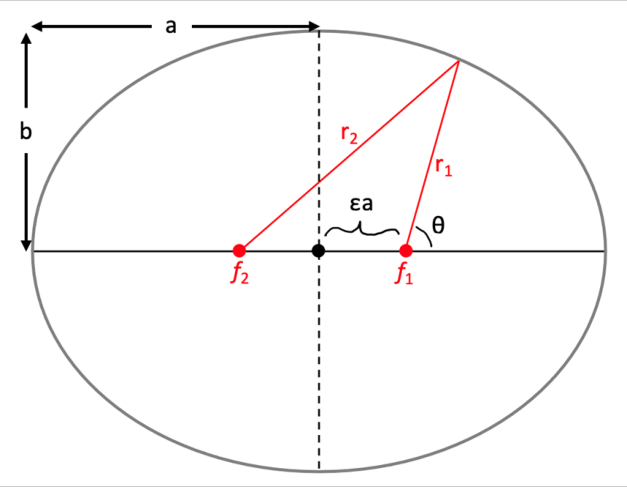
Figure 11.1 shows an example ellipse with several key properties labeled. An ellipse is essentially an elongated circle, where the longer of the two axes is the semi-major axis $(a)$ and the shorter of the two axes is the semi-minor axis $(b)$ . The degree to which the circle has been stretched is called the eccentricity (or ellipticity) and is denoted by the symbol $\varepsilon$ ,

\varepsilon=\sqrt{1-\frac{b^2}{a^2}}.

(1)

Figure 11.1 also shows two special points in red, which are called the foci (focus is the singular term). These two foci, denoted as $f_{1}$ and $f_{2}$ , are located on the semi-major axis, each at a distance $\varepsilon a$ from the center of the ellipse. The foci of an ellipse define the shape. An ellipse is defined by a locus (path) of points where the total distance from any point on

the locus to the two foci adds up to a constant. For example, Figure 11.1 shows a point on the ellipse that is a distance $r_{1}$ from $f_{1}$ and a distance $r_{2}$ from $f_{2}$ . The shape of the ellipse is defined such that the sum of those two distances $r_{1}+r_{2}$ = constant for every position on the locus. For an ellipse, $r_{1}+ r_{2}= 2a$ .

Figure 11.1 from the source textbook — Figure 11.1:Schematic of an ellipse. The center is shown by a black dot and the two foci are shown as red dots. The semi-major axis $(a)$ and semi-minor axis $(b)$ are also labeled. The two foci are each a distance $\varepsilon a$ from the center, where $\varepsilon$ is the eccentricity. The total distance between the two foci $(r_{1}$ and $r_{2})$ and any position on the ellipse sum to a constant, $r_{1}+ r_{2}$ = constant.

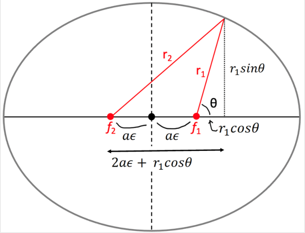
The distances $r_{1}$ and $r_{2}$ in Figure 11.1 can be measured relative to $a, \varepsilon$ , and a position angle, $\theta$ . Figure 11.2 shows how we can relate these properties through Pythagoras’ theorem. Using the right-angle triangle in Figure 11.2, we have

r_{2}^{2}= (r_{1}\sin \theta)^{2}+ (2a\varepsilon + r_{1}\cos \theta)^{2}

(2)

Expanding on this, we get

\begin{aligned} r_2^2&=r_1^2\sin^2\theta+4a^2\varepsilon^2+4a\varepsilon r_1\cos\theta+r_1^2\cos^2\theta\\ &=r_1^2(\sin^2\theta+\cos^2\theta)+4a\varepsilon(a\varepsilon+r_1\cos\theta). \end{aligned}

(3)

r_{2}^{2}= r_{1}^{2}+ 4a\varepsilon (a\varepsilon + r_{1}\cos \theta)

(4)

Finally, we can use the property that $r_{2}+ r_{1}= 2a$ for an ellipse.

\begin{aligned} (2a - r_{1})^{2}&= r_{1}^{2}+ 4a\varepsilon (a\varepsilon + r_{1}\cos \theta) \\ 4a^{2}- 4ar_{1}+ r_{1}^{2}&= r_{1}^{2}+ 4a\varepsilon (a\varepsilon + r_{1}\cos \theta) \\ -4ar_{1}&= 4a\varepsilon (a\varepsilon + r_{1}\cos \theta) - 4a^{2} \end{aligned}

(5)

r_{1}= -a\varepsilon ^{2}- r_{1}\varepsilon \cos \theta + a

(6)

r_{1}(1 + \varepsilon \cos \theta) = a(1 - \varepsilon ^{2})

(7)

r_{1}= \frac{a(1 - \varepsilon ^{2})}{1 + \varepsilon \cos \theta}

(8)

Figure shows the vector breakdown for a locus on an ellipse in terms following standard Cartesian coordinates. — Figure 11.2:This shows the position vectors $r_{1}$ and $r_{2}$ again for the two foci, where $r_{1}$ has been broken up into two components, $r_{1}\sin \theta$ and $r_{1}\cos \theta$ . This produces a right angle triangle with $r_{2}^{2} = (r_{1}\sin \theta)^{2}+ (2a\varepsilon + r_{1}\cos \theta)^{2}$ using the Pythagorean theorem.

Now we don’t need to use the subscript for $r$ . We can say that the distance to any point on the ellipse from a given focus is:

r = \frac{a(1 - \varepsilon ^{2})}{1 + \varepsilon \cos \theta}

(9)

For our elliptical orbit, $r$ is the distance from one of the foci to the ellipse as a function of the angle. We define $\theta$ = 0 along the semi-major axis (e.g., see Figure 11.1 for the definition of the angle). Since $-1 \le \cos \theta \le 1$ , the distance from the focus is smallest when $\theta = 0^{\circ}$ and largest when $\theta = 180^{\circ}$ .

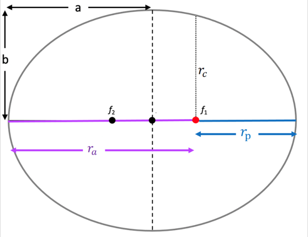
Figure 11.3 shows the definition of these closest and farthest points. This shortest distance from the focus is called the pericenter $(r_{p})$ and is shown in blue. The largest distance from the focus is called the apocenter $(r_{a})$ and it is shown in purple. The pericenter and apocenter distances are defined as:

r_{p}= a(1 - \varepsilon)

(10)

r_{a}= a(1 + \varepsilon)

(11)

Figure shows an ellipse representing an orbit with the apocenter and pericenter distances and the semi-major and semi-minor axes labeled. — Figure 11.3:The apocenter $r_{a}$ and pericenter $r_{p}$ for an ellipse. Also shown is $r_{c}$ the distance between the focus and locus at an angle that is perpendicular to the semi-major axis $(\theta = 90^{\circ})$ .

Pericenter and Apocenter

For an elliptical orbit, the pericenter and apocenter are special places where $\dot{r}$ = 0. These are otherwise known as turning points. You are moving from a case of increasing radius (pericenter to apocenter) to a case of decreasing radius (apocenter to pericenter). So at these specific points, $\dot{r}$ is instantaneously zero.

If it helps, consider simple harmonic motion as an analogy. For a pendulum that is oscillating, the maximum amplitude $\theta _{\max}$ occurs when $K$ = 0. At that point, the system starts moving back in the opposite direction. So the maximum displacement is $\theta _{\max}$ when the kinetic energy is zero. For an elliptical orbit, the apocenter and pericenter are the equivalent of our turning points and they represent the maximum and minimum distances of the orbit.

In general, we use the term perigee for the pericenter and apogee for the apocenter when talking about orbits around the Earth, and perihelion and aphelion for the pericenter and apocenter of orbits around the Sun.

11.2 Ellipses as Orbits¶

The previous section defines the ellipse as a geometric shape. Now we will put some physics into the elliptical orbit so we can relate the motion of an object in a gravitational field.

Gravity is a central force that follows an inverse-square law. In Chapter 10, we showed that the energy of a system under a central force has the form of

E = \frac{1}{2} m\dot{r}^{2}+ U_{eff}

(12)

where $U_{eff}$ is the effective potential. Since we are interested in orbits under gravity, we can define the effective potential as

U_{eff}= \frac{1}{2} \frac{L^{2}}{mr^{2}} - \frac{\gamma}{r}

(13)

where $L = mr^{2}\dot{\theta}$ is the angular momentum and $\gamma = GMm$ . For central forces like gravity, $L$ = constant.

Starting from these equations, we must solve for $r(\theta)$ to describe the orbit. The full derivation of this solution is given in Appendix B.1. It is a good exercise of your understanding if you can follow how we go from the two previous equations to the next equation.

Taking the equations for a central force, $r(\theta)$ is:

r(\theta)=\left(\frac{L^2}{m\gamma}\right) \frac{1}{1+\sqrt{1+\frac{2EL^2}{m\gamma^2}}\cos\theta}.

(14)

The above equation has the same form as a general ellipse (Equation 11.2). This indicates that our solution for a central force is an ellipse. Moreover, we can define $\varepsilon$ from the physics as

\varepsilon=\sqrt{1+\frac{2EL^2}{m\gamma^2}}.

(15)

Note that for the orbit to be a true ellipse, we need 0 $< \varepsilon < 1$ . This condition is only met if $E < 0$ , which was the same conclusion that we obtained in Chapter 10 when we looked at the energy and found that $r$ had two real solutions when $E < 0$ .

In Chapter 10.6, we showed that a circular orbit occurs when the energy of the system equals the local minimum of the effective potential. The radius of this circular orbit is

r_{c}= \frac{L^{2}}{m\gamma}

(16)

for the gravitational force. We can also prove this definition of $r_{c}$ using Newton’s laws for uniform circular motion.

\begin{aligned} \frac{\gamma}{r_{c}^{2}} &= \frac{mv^{2}}{r_{c}} =\Rightarrow \gamma r_{c}= mv^{2}r_{c}^{2} \\ r_{c}&= \frac{(mvr_{c})^{2}}{m\gamma} =\Rightarrow L = mvr_{c} \end{aligned}

(17)

r_{c}= \frac{L^{2}}{m\gamma}

(18)

So $r_{c}$ is the radius of a circular orbit with an angular momentum of $L = mvr_{c}$ .

Combining Equations 11.5 and 11.6 with the equation for $r(\theta)$ , we can describe a position on the orbit as,

r(\theta) = \frac{r_{c}}{1 + \varepsilon \cos \theta}

(19)

There are different kinds of orbits. For $\varepsilon < 1$ , the orbit is elliptical, with the special case of $\varepsilon$ = 0 for perfectly circular orbits. These are the only orbits we will deal with in great detail in this textbook.

For elliptical orbits, we define the pericenter and apocenter as the positions of closest and furthest distance from one of the foci. In terms of the physics of the system, we want to relate the pericenter and apocenter to $r_{c}$ , because $r_{c}$ contains our physics.

r = \frac{r_{c}}{1 + \varepsilon \cos \theta}

(20)

The pericenter is the closest position and it corresponds to $\theta$ = 0 and the apocenter is the furthest position when $\theta = 180^{\circ}$ . Putting these cases into $r$ , we get:

r_{p}= \frac{r_{c}}{1 + \varepsilon}

(21)

r_{a}= \frac{r_{c}}{1 - \varepsilon}

(22)

For $\varepsilon \ge 1$ , the orbit is unbound. These are hyperbolic orbits $(\varepsilon > 1)$ or parabolic orbits $(\varepsilon$ = 1). The above equations for the pericenter and apocenter show that this must be true. As $\varepsilon \rightarrow$ 1, the apocenter distance becomes $r_{a}\rightarrow \infty$ . That means that your furthest distance is moving so far away that the object is no longer bound to your gravitational field. If you are not bound to the gravitational field, then your system has too much energy to be contained by that field and it will just come in and go out.

a) First, let’s consider the initial energy of the satellite. Since the satellite starts in a circular orbit, we know that $\dot{r}$ = 0 for the full orbit (radius does not change) and the system energy equals the minimum of the effective potential. From Chapter 10.6, the radius and energy of a circular orbit are:

r_{c}= \frac{L^{2}}{m\gamma}

(23)

E_{\min}= - \frac{1}{2} \frac{m\gamma ^{2}}{L^{2}}

(24)

So our initial energy is $E_i=-m\gamma^2/(2L^2)$ .

Now, let’s consider what happens to the energy after the engines are fired briefly. We will first assume that the satellite moves a negligible amount, so its position vector, $r$ is unchanged during the energy boost from the engines. We are told that the energy is directed inward toward the Earth. In other words, the energy is applied along a radial direction. Any motion along the radial direction does not change the angular momentum, because $L = \vec{r} \times \vec{p}$ . The component of motion along a radial direction does not produce additional angular momentum. So $L$ is the same before and after the energy boost. Thus, the effective potential does not change.

But, the energy boost does induce a change in the radial momentum, which means that $\dot{r} \not =$ 0. If we have a radial velocity, then our energy after the boost, $E_{f}$ is

E_{f}= \frac{1}{2} m\dot{r}^{2}+ U_{eff}

(25)

Since the effective potential is unaltered by the engine boost, we can re-write $U_{eff}$ as $E_{i}$ , since $E_{i}= U_{eff}$ before the engines fired.

E_{f}= \frac{1}{2} m\dot{r}^{2}+ E_{i}

(26)

Thus, the total energy has increased because kinetic energy was added to the satellite. It does not matter if the rockets move the satellite toward the Earth $(\dot{r} < 0)$ or away from the Earth $(\dot{r} > 0)$ , the kinetic energy term is always positive so it will always add to the total energy. The final energy, $E_{f}$ , must be larger than our initial energy $E_{i}$ . The exact value larger depends on the radial velocity $\dot{r}$ given to the satellite by the engines. Since we are not given that quantity, all we can conclude is that the total energy of the satellite has increased due to the engines firing.

b) There are a couple of ways we can answer this question. First, we can sketch the energy diagram. Figure 11.4 shows a sketch of what the initial and final energies may

Continued

look like for this satellite. Note, we are assuming that the boost in energy is sufficiently small that the satellite remains bound to the Earth.

Figure 11.4:Change in energy for our perturbed satellite. The satellite starts in a circular orbit so that $E = E_{i}$ which is at the minimum of the effective potential. After the engines are fired, the energy increases so that $E = E_{f}$ .

Figure 11.4 shows the initial energy, $E_{i}$ at the minimum of $U_{eff}$ and the final energy $E_{f}$ which is somewhat larger. The increase in energy makes the satellite go into an elliptical orbit. We can see that the orbit is elliptical because we have two solutions for $r$ when the energy line hits the effective potential curve (denoted by $r_{1}$ and $r_{2}$ in the figure). These values of $r_{1}$ and $r_{2}$ are the perigee and apogee positions of the satellite (with the Earth at a focus). If the engines move the rocket inward initially, the rocket will begin moving toward its perigee position (from an initially circular orbit of $r_{c}$ ).

Alternatively, we could argue that the orbit is elliptical by looking at the equation for $\varepsilon$ in Equation 11.5. From this equation, $\varepsilon$ = 0 when $E = E_{\min}$ and $\varepsilon$ will increase if $E > E_{\min}$ . An orbit is circular if $\varepsilon$ = 0 and elliptical for 0 $< \varepsilon < 1$ .

11.3 Kepler’s Laws¶

Kepler introduced three laws to describe planetary motion. These were based on careful observations by astronomer Tycho Brahe. Kepler used the systematics of these observations to determine how planets move. About 80 years later, Newton was able to explain this planetary motion using the physics of gravity.

The three laws of planetary motion are:

Planets move on elliptical orbits with the Sun at one focus.
The vector from the Sun to a planet sweeps out equal areas in equal times.
The square of the period of a full orbit about the Sun is proportional to the cube of the semi-major axis.

For the first law, we have shown in this chapter (and in the last chapter) that bound orbits are elliptical in a gravitational potential (we consider circular orbits to be a special case of the elliptical orbit where $r_{p}= r_{a})$ . Gravity being a central force that follows an inverse-

square law will naturally give rise to elliptical orbits provided that the system is bound.

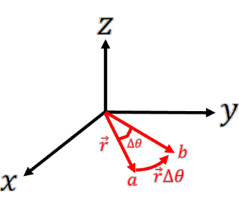
For the second law, the radius vector from the Sun sweeps equal areas in equal times because of the conservation of angular momentum. Recall also that for a central force, all motion takes place in a 2-D plane (see Chapter 10). Thus, we can use plane polar coordinates to describe the motion alone. Figure 11.5 shows the area swept out by the radius vector in time $\Delta t$ in polar coordinates.

Figure shows a standard set of 3d Cartesian axes with a vector sweeping out an area between two points. — Figure 11.5:Motion in the $xy$ plane from a central force. In time $\Delta t$ , the object moves from position $a$ to position $b$ and sweeps out an area defined by the triangle from the origin to $a$ and $b$ .

In time $\Delta t$ , a particle moves from position $a$ to position $b$ as shown in Figure 11.5. The area (from the origin) to those points is a triangle with

\begin{aligned} \Delta A &= \frac{1}{2} r(r\Delta \theta) = \frac{r^{2}\Delta \theta}{2} \\ \frac{\Delta A}{\Delta t} &= \frac{r^{2}}{2} \frac{\Delta \theta}{\Delta t} =\Rightarrow \mathrm{divide} \mathrm{both} \mathrm{sides} \mathrm{by} \Delta t \end{aligned}

(27)

Note that this assumes that you have small enough angles $\Delta \theta$ so that we can approximate the area as a triangle. This approximation is true for infinitesimally small times. Therefore, we can assume $\Delta t \rightarrow$ d $t, \Delta A \rightarrow$ d $A$ , and $\Delta \theta \rightarrow$ d $\theta$ .

\begin{aligned} \frac{\mathrm{d}A}{\mathrm{d}t} &= \frac{r^{2}}{2} \frac{\mathrm{d}\theta}{\mathrm{d}t} \\ \dot{A} &= \frac{r^{2}\dot{\theta}}{2} =\Rightarrow \mathrm{recall} L = mr^{2}\dot{\theta} \\ \dot{A} &= \frac{L}{2m} =\Rightarrow L = \mathrm{constant} \\ \dot{A} &= \mathrm{constant} \end{aligned}

(28)

Because we have a constant angular momentum, we naturally get Kepler’s second law that equal areas are swept out in equal time intervals (or $\dot{A}$ = constant).

For the third law, we have:

\frac{T^{2}}{a^{3}} = \mathrm{constant}

(29)

where $T$ is the period and $a$ is the semi-major axis. To show this is the case, we need to use the previous laws and our equations for the properties of an ellipse.

From the second law, $\dot{A}$ is a constant. So we know the speed by which we trace out an area in our ellipse. The total area of an ellipse is just $A_{tot}= \pi ab$ , where $a$ and $b$ are the semi-major and semi-minor axes. Thus, the period can be given as:

T = \frac{A}{\dot{A}} = \frac{\pi ab}{L/2m} = \frac{2\pi mab}{L}

(30)

We also can relate the semi-major and semi-minor axes to each other: $b=a\sqrt{1-\varepsilon^2}$ . Now we need to get $1-\varepsilon^2$ in terms of $a$ and the physics. From Equations (11.8) and (11.9)

\begin{aligned} r_{p}&= \frac{r_{c}}{1 + \varepsilon} \\ r_{a}&= \frac{r_{c}}{1 - \varepsilon} \end{aligned}

(31)

We also know that $r_{p}+ r_{a}= 2a$ for an ellipse. Therefore, we can add the above equations to give:

\begin{aligned} r_{p}+ r_{a}&= 2a \\ 2a &= \frac{r_{c}}{1 + \varepsilon} + \frac{r_{c}}{1 - \varepsilon} \\ 2a &= r_{c}\bigg(\frac{1 - \varepsilon}{1 - \varepsilon ^{2}} + \frac{1 + \varepsilon}{1 - \varepsilon ^{2}} \bigg) \\ 2a &= r_{c}\bigg(\frac{2}{1 - \varepsilon ^{2}} \bigg) \\ 1 - \varepsilon ^{2}&= \frac{r_{c}}{a} =\Rightarrow r_{c}= \frac{L^{2}}{m\gamma} \end{aligned}

(32)

1 - \varepsilon ^{2}= \frac{L^{2}}{am\gamma}

(33)

Thus, we can re-write the period equation as:

\begin{aligned} T&=\frac{2\pi mab}{L}\\ &=\frac{2\pi ma^2\sqrt{1-\varepsilon^2}}{L}\\ &=\frac{2\pi ma^2\sqrt{L^2/(am\gamma)}}{L},\\ T^2&=\frac{4\pi^2m^2a^4(L^2/(am\gamma))}{L^2} =\frac{4\pi^2ma^3}{\gamma}. \end{aligned}

(34)

T^{2}= \frac{4\pi ^{2}a^{3}}{GM} =\Rightarrow \mathrm{sub} \gamma = GMm

(35)

\frac{T^{2}}{a^{3}} = \frac{4\pi ^{2}}{GM} = \mathrm{constant}

(36)

11.4 Application of Kepler’s Laws¶

Here we will look at a few problems that apply Kepler’s Laws.

set $M = M_{sun}= 2.0 \times 10^{30}$ kg. Plugging in our numbers, we get:

[75\,\mathrm{years} \times (3.154 \times 10^{7}\,\mathrm{s/year})]^{2} = \frac{4\pi^{2}a^{3}}{(6.67\times10^{-11}\,\mathrm{m^{3}\,kg^{-1}\,s^{-2}})(2.0\times10^{30}\,\mathrm{kg})}.

(38)

5.6 \times 10^{18}\mathrm{s}^{2}= (2.97 \times 10^{-19}\mathrm{s}^{2}\mathrm{m}^{-3})a^{3}

(39)

a^{3}= 1.9 \times 10^{40}\mathrm{m}^{3}

(40)

a = 2.66 \times 10^{12}\mathrm{m}

(41)

a = 18 \mathrm{au}

(42)

Now this is a perfectly acceptable way to solve the problem, but it involves a lot of math and plugging big numbers into a calculator. It is easy to make a mistake with that. A better way to solve this problem is to use scaling relations.

From the third law, $T^2\propto a^3$ , or $T^2/a^3=$ constant. That means if we know $T$ and $a$ for one orbit, we can scale that solution to correspond to any other orbit around the same object. Consider two objects orbiting the Sun. The first object has a period $T_1$ and a semi-major axis $a_1$ ; the second object has a period $T_2$ and semi-major axis $a_2$ . Since

T^{2}\propto a^{3},

(43)

\bigg(\frac{T_{1}}{T_{2}} \bigg)^{2}= \bigg(\frac{a_{1}}{a_{2}} \bigg)^{3}

(44)

This is a scaling relation. It is a much simpler (and faster) way to solve the same problem. As long as you have a reference system, you can scale that reference system to any other orbit that goes around the same body. A convenient reference system is the Earth. We know that it takes 1 year for the Earth to orbit the Sun and the Earth by definition is 1 au from the Sun. So our scaling relation becomes:

\Bigg(\frac{T}{1 \mathrm{year}} \Bigg)^{2}= \bigg(\frac{a}{1 \mathrm{au}} \bigg)^{3}

(45)

With this scaling relation, let’s go back to our question about Halley’s comet. Halley’s comet has a period of 75 years.

\begin{aligned} \Bigg(\frac{75 \mathrm{years}}{1 \mathrm{year}} \Bigg)^{2}&= \bigg(\frac{a}{1 \mathrm{au}} \bigg)^{3} \\ \bigg(\frac{a}{1 \mathrm{au}} \bigg) &= 75^{2/3} \\ a &= 18 \mathrm{au} \end{aligned}

(46)

Look at how much faster it was to solve the same problem using a scaling relation. You get the same answer, but the math is much simpler. You can also make quick comparisons between systems using scaling relations, which makes these approaches to solving problems very efficient.

Continued

Note, the above scaling relation only applies to orbits around the Sun. If you change the source of the gravitational field, you need to change your reference orbit. This is because the constant of proportionality between $T^{2}$ and $a^{3}$ depends on the mass, $M$ , that is producing the gravitational field.

Scaling relations, like the one used in this question, can be extremely useful. In the astrophysics field, scaling relations are often used to describe trends observed between physical properties such as size, luminosity, mass, and colour of stars and galaxies. It can be very hard to determine these properties due to the large distances, gas clouds, and other factors in space. So, scaling relations such as the Faber-Jackson Relation (FJR) are used to determine these physical properties that are otherwise difficult to obtain or compare.

Sample Problem 11-3

Halley’s comet has an eccentricity of $\varepsilon = 0.967$ . What are the perihelion and aphe- lion distances and how fast is the comet traveling at those positions?

Solution

Perihelion and aphelion are the terms used for the pericenter and apocenter when the Sun is at the focus. From Equations (11.3) and (11.4) and the semi-major axis of 18 au for Halley’s comet from the last problem, we can easily solve for $r_{p}$ and $r_{a}$ .

r_{p}= a(1 - \varepsilon) = (18 \mathrm{au})(1- 0.967) = 0.6 \mathrm{au}

(47)

r_{a}= a(1 + \varepsilon) = (18 \mathrm{au})(1 + 0.967) = 35 \mathrm{au}

(48)

To get the speeds at perihelion and aphelion, let’s start with the angular momentum. At these positions, the radial vectors and velocity vectors are perpendicular $(\dot{r}$ is zero). Thus,

L = mv_{a}r_{a}= mv_{p}r_{p}

(49)

which is a constant. We can also relate $L$ to the equivalent radius for a circular orbit, $r_{c}$ , and we can relate $r_{c}$ to the perihelion and aphelion distances.

Continued

\begin{aligned} r_{c}&= \frac{L^{2}}{m\gamma} \\ r_{p}&= \frac{r_{c}}{1 + \varepsilon} \\ r_{a}&= \frac{r_{c}}{1 - \varepsilon} \end{aligned}

(50)

Plugging these in with the angular momentum equation,

\begin{aligned} mv_pr_p&=\sqrt{r_cm\gamma}=\sqrt{(1+\varepsilon)r_pm\gamma},\\ v_p&=\sqrt{\frac{(1+\varepsilon)\gamma}{r_pm}} =\sqrt{\frac{GM(1+\varepsilon)}{r_p}}. \end{aligned}

(51)

Follow the same procedure for the aphelion distance to get

v_a=\sqrt{\frac{GM(1-\varepsilon)}{r_a}}.

(52)

Since we are interested in speeds, we do not care about the negative signs with the square root.

If we plug in our values for $M, \varepsilon, r_{a}$ and $r_{p}$ into the above equations, we get:

v_{p}= 55 \mathrm{km} \mathrm{s}^{-1}

(53)

v_{a}= 0.9 \mathrm{km} \mathrm{s}^{-1}

(54)

As expected, we get $v_{p}> v_{a}$ .

Prove that $v_a=\sqrt{GM(1-\varepsilon)/r_a}$ .
Show that $v_{p}$ = 55 km $\mathrm{s}^{-1}$ and $v_{a}= 0.9$ km $\mathrm{s}^{-1}$ for Halley’s comet.

11.5 Real World Application¶

Preventing an asteroid strike on Earth may seem like a plot out of a movie, but there is ongoing research into how to do this properly. Rather than trying to blow up the asteroid, scientists have come up with different technique: alter the orbit through a kinetic impact. The basis of this plan is to slam a spacecraft into an asteroid head on so that it loses angular momentum and subsequently moves into a slightly different orbit.

The Double Asteroid Redirection Test (DART) spacecraft was launched to test this exact scenario. DART targeted a tiny asteroid called Dimorphos, which is in orbit around a larger asteroid, Didymos. The goal of this mission was to use the kinetic impact of DART to change the orbital parameters of Dimorphos.

On 26 September 2022, DART made impact on Dimorphos and successfully caused the moonlet to spiral inward into a new (smaller) orbit. Subsequent observations confirmed a new orbital period that decreased by 32 minutes (from an original length of almost 12 hours). The mission was a big success and showed that such techniques could be used to protect the Earth in future.

For more information: The DART Mission Website has lots of information and there is also video of the impact. The Jet Propulsion Lab some information on the science and engineering behind the mission.

11.6 Summary¶

Key Takeaways

This chapter expands on orbits from Chapter 10, describing and defining the geometric shapes and physics of elliptical orbits. Ellipses are elongated circles of semi-major axis $a$ , semi-minor axis $b$ , and eccentricity $\varepsilon$ . Mathematically, these shapes are defined as:

r = \frac{a(1 - \varepsilon ^{2})}{1 + \varepsilon \cos \theta}

(55)

\varepsilon=\sqrt{1-\frac{b^2}{a^2}}.

(56)

where $r$ is measured from one of the two foci of the ellipse. The closest point of an ellipse to the focus is called the pericenter and the furthest point is called the apocenter:

r_{p}= a(1 - \varepsilon)

(57)

r_{a}= a(1 + \varepsilon)

(58)

For a system with only gravity acting, we derived the orbit equation in terms of the the

Continued

angular momentum $L$ and total energy $E$ ,

r = \frac{L^{2}/(m\gamma)}{1 + \varepsilon \cos \theta}

(59)

\varepsilon=\sqrt{1+\frac{2EL^2}{m\gamma^2}}.

(60)

and we defined a radius, $r_{c}$ , which represents the radius of a circular orbit for a system of angular momentum $L$ and $E = E_{\min}$ .

r_{c}= \frac{L^{2}}{m\gamma}

(61)

Note that $E \ge U_{eff}$ for a gravitational field, because gravity is a central force. Thus, a key element to the shape of an orbit is the amount of energy in the system. If there is the minimum energy, the orbit is circular. As the energy increases, the orbit becomes elliptical and then unbound (parabolic or hyperbolic).

This chapter also discusses Kepler’s three laws of planetary motion. These laws apply to orbits because gravity is a central force with an inverse-square law. The most applicable law is the third law, where

\frac{T^{2}}{a^{3}} = \frac{4\pi ^{2}}{GM} = \mathrm{constant}

(62)

A useful technique when applying Kepler’s third law is to use scaling relations. If you know a solution for one case of $T$ and $a$ , you can scale to any other case of $T$ or $a$ for the same gravitational field.

11.7 Practice Problems¶

See Appendix C for answers to the practice problems.