B. Derivations and Approximations

B.1 Derivation of Elliptical Orbits¶

Starting from the energy equation for a central force (Chapter 10), we have

where $U_{eff}$ is the effective potential. Re-arranging the equation gives:

where $\dot{r} = \frac{\mathrm{d}r}{\mathrm{d}t}$. We want to get $r(\theta)$ to describe the orbit. To do this, we will use the ratio of $\dot{r}$ and $\dot{\theta}$ ,

So we need to get an equation for $\dot{\theta}$ .

For $\dot{\theta}$ , we can use the conservation of angular momentum. Recall that central forces conserve angular momentum by definition (see Chapter 10). The magnitude of angular momentum is:

with $L$ = constant.

We can then combine the $\dot{r}$ and $\dot{\theta}$ equations as follows:

Equation B.4 applies to any effective potential. Since we’re talking about orbits, the central force is gravity. That makes the effective potential:

where $\gamma = GMm$ for simplicity. Substituting Equation B.5 into Equation B.4 gives,

To solve Equation B.6, there is a substitution trick we can use to help simplify the problem. Instead of solving for $r$, we’re going to solve for $y = \frac{1}{r}$. The reason for this substitution is that

Thus, we can write Equation B.6 in terms of $y = \frac{1}{r}$ instead of $r$.

Already this looks simpler. We can simplify more, however, by “completing the square”,

Note that the first two terms on the righthand side of Equation 8 are present in the righthand side of Equation B.7. From Equation B.8, we can say that

And we can substitute Equation B.9 into Equation B.7 to give:

With Equation B.10, we have an equation with one $y$ term and two constant terms. To make the equation a bit simpler, we will introduce a couple more substitutions for the constants.

First, we will use $z = y - \dfrac{m\gamma}{L^{2}}$. Note that $\dfrac{\mathrm{d}z}{\mathrm{d}\theta} = \dfrac{\mathrm{d}y}{\mathrm{d}\theta}$ because $\dfrac{m\gamma}{L^{2}}$ is a constant.

Second, we will substitute for the sum of the remaining constants as $B^{2}$,

Substituting Equation B.12 into Equation B.11, we get:

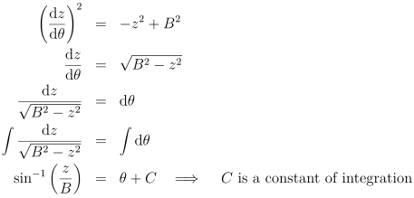
Now we have a fairly straightforward integral to solve. The solution to this problem is available in Appendix A.

We can select the initial conditions such that the initial angle is anything we want because the motion is periodic. For ellipses, it helps to have the angle in terms of cos instead of sin, so we can set $C = \frac{\pi}{2}$. Thus, we get the solution:

Now we need to put back all of those substitutions that we made!

3. From Equation B.13: $B = \dfrac{m\gamma}{L^{2}}\sqrt{1 + \dfrac{2EL^{2}}{m\gamma^{2}}}$

We now define the eccentricity of the orbit, $\varepsilon$ as:

Substitute Equation B.16 into Equation B.15:

Finally, let’s solve for $r$.

We now have an equation of $r(\theta)$ that defines our orbit. You will note that Equation B.18 has a similar structure to the equation for a generic ellipse (Equation 11.2), but with different constants out front.

If $\varepsilon$ = 0, then we have a circular orbit with a radius of

We define $r_{c}$ as the radius of a circular orbit for a given angular momentum, $L$. See also Chapter 11.2 for the derivation of $r_{c}$ using Newton’s laws.

So substituting in $r_{c}$, we recover Equation 11.7.

B.2 Approximations¶

Many times, mathematical functions can be simplified by using limits and making reasonable approximations. There are many ways to simplify a function. Here, we will look at a few of them.

B.2.1 Binomial Approximation¶

For simple power functions, such as $f(x)$ = (1 + $x)^{a}$, you can apply the binomial or linear expansion to approximate their value. The approximation works as follows:

where $x_{0}$ is the point about which you are measuring $x$. That is, you are expanding the series about the point where $x = x_{0}$.

At first glance, this approximation seems reasonable. The approximation states that the value of a function at position $x$ near position $x_{0}$ can be approximated by the value at position $x_{0}$ with a modification given by the slope at $x_{0}$ and the distance between $x_{0}$ and $x$. For values of $x \approx x_{0}$, this approximation should be reasonable.

For the function, $f(x)$ = (1 + $x)^{a}$ with $x_{0}$ = 0, the binomial approximation would be,

In this case, the value of $x$ must be close to zero for the approximation to be valid. If $x$ is not close to zero, then we need to shift $x_{0}$.

B.2.2 Taylor Series¶

For more general functions, you can approximate the function using its Taylor series,

where $x_{0}$ = 0 has the same meaning as before.

For example, the Taylor series expansion of $\sqrt{1 + x}$ (where $x_{0}$ = 0) is equal to:

If $x$ is small $(x$ is close to zero), then $x^{2}$ and $x^{3}$ are very small and don’t change the result much. For example, if $x = 0.1$, then $x^{3}= 0.001$ and $\frac{1}{16} x^{3}= 6.25\times 10^{-5}$. That term is much smaller than 1 and all subsequent terms will be even smaller, so they are negligible. That means, for small values of $x$, we can approximate $\sqrt{1 + x}$ as:

It is key that $x$ is small (for $x_{0}$ = 0). If $x$ is larger, then the higher order terms are more significant and cannot be considered negligible.

The Taylor series for the $\sin x$ and $\cos x$ (with $x_{0}$ = 0) are:

Note that $x$ must be in radians for the Taylor series approximation to hold. You cannot use $x$ in degree. If $x$ (in radians) is small, then the higher order terms again become negligible and $\sin x \approx x$ and $\cos x \approx 1 - \frac{x^{2}}{2}$ . There are several functions with well established Taylor series approximations based on the above definition. Appendix A.3 lists the expansions for many common equations.