3. Simple Harmonic Motion - Second-Year Dynamics

In this chapter, we will apply Newton’s Laws to cases of simple harmonic motion.

3.1 Force is Proportional to Position¶

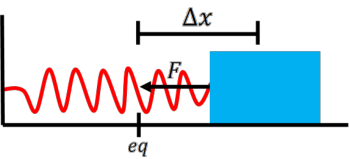
Let’s consider a force that is proportional to the position of the system. Examples of such forces are found in springs, pendulums, and torsion oscillators. Figure 3.1 shows a case of a spring and mass, where the force acting on the mass from the spring is $F = -kx$ , where $k$ is a positive constant. (Note this equation is also called Hooke’s Law.)

Figure shows a mass attached to a spring on a horizontal surface. — Figure 3.1:Example of the spring force acting on a mass.

A force in the form of $F = -kx$ is also called a restoring force, because the force seeks to return a system to a state of equilibrium $(x$ = 0). For example, in Figure 3.1, the spring is stretched from where it wants to be, $x_{0}$ . The spring force will try to return the mass back to its equilibrium state.

If the net force acting on the mass is the spring force, then we can use Newton’s second law, $\sum F = ma = -kx$ to get,

a = \frac{\mathrm{d}^{2}x}{\mathrm{d}t^{2}} = - \frac{k}{m} x

(1)

Equation 3.1 is a second-order differential equation, where the second time derivative of displacement is proportional to the displacement $(k$ and $m$ are constants). Thus, we need a function that when differentiated twice gives you the negative of that original function multiplied by a constant. This type of problem has a well known solution. Two familiar functions that meet these conditions are the cos and sin functions.

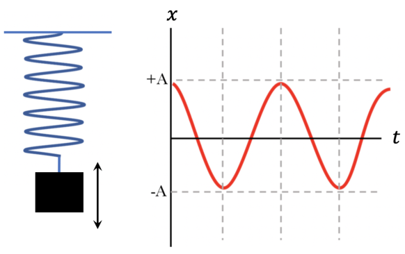
The solution of a $\cos t$ or $\sin t$ function should make sense. Picture a mass hanging from a spring. If you move the mass upward and let go, the mass will initially move downwards until it reaches a maximum drop at which point it will be pulled back upwards until it reaches its original position then it will move back downwards. Essentially, the mass will move down and up in a periodic manner. Figure 3.2 shows the up-down displacement of this mass as a function of time; note that the displacement looks like a cos (or sin) function.

Figure shows a cartoon of a mass hanging from a vertical spring next to a graph showing the periodic displacement of the mass over time. — Figure 3.2:Motion of a simple harmonic oscillator. The left panel shows that the mass will move up and down in periodic motion. The right panel shows a sketch of its displacement over time. The mass starts with a maximum displacement (e.g., maximum compression of the spring) and moves to the other end (e.g., maximum extension of the spring) and back again. This back-and-forth motion continues.

Therefore, the solution to the second-order differential equation (Eq 3.1) is met with:

x = A\cos (\omega _{0}t + \varphi)

(2)

where $A,\omega _{0}$ , and $\varphi$ are all constants.

$A$ is the amplitude of the motion, the maximum displacement from equilibrium.
$\omega _{0}$ is the angular frequency. This is not the same as angular velocity (recall that we used $\omega = \frac{\mathrm{d}\theta}{\mathrm{d}t})$ . Instead, $\omega _{0}$ is a fundamental property of the system itself. See details below for more details.
$\varphi$ is the phase constant (sets where you are in the motion at $t$ = 0).

Equation 3.2 is a generic solution to the second-order differential equation that works for any simple harmonic oscillator (not just a mass and spring). Note also that instead of cos, we can use $B\sin (\omega _{0}t + \varphi _{2})$ , where $B,\omega _{0}$ , and $\varphi _{2}$ are all constants. Indeed, the cos and sin forms of the equation are interchangeable if you just alter the value of the phase constant. In practice, the most general solution for simple harmonic motion would be a superposition of cos and sin functions. For this textbook, however, we will assume that the motion can be described via a single periodic function and we will use the cos function by default.

Now that we have $x(t)$ , we just need to differentiate once to get the velocity.

\begin{aligned} v&=\dot{x} \\ v&=\frac{\mathrm{d}}{\mathrm{d}t}\left[A\cos(\omega_{0}t+\varphi)\right] \end{aligned}

(3)

v = -\omega _{0}A\sin (\omega _{0}t + \varphi)

(4)

And we can differentiate again to get the acceleration.

\begin{aligned} a&=\dot{v} \\ a&=\frac{\mathrm{d}}{\mathrm{d}t}\left[-\omega_{0}A\sin(\omega_{0}t+\varphi)\right] \\ a&=-\omega_{0}^{2}\underbrace{\left[A\cos(\omega_{0}t+\varphi)\right]}_{x(t)} \end{aligned}

(5)

a = -\omega _{0}^{2}x

(6)

Thus, we find that $a = -\omega _{0}^{2}x$ , where $\omega _{0}$ is the angular frequency constant. Going back to our original definition of the force in Equation (3.1), we had $a = - \frac{k}{m} x$ for the force $F = -kx$ . Thus, the generic differential equation of motion solves Hooke’s Law if:

\omega_{0}=\sqrt{\frac{k}{m}}

(7)

Note that for other restoring forces, the solution for $\omega _{0}$ will be different.

3.2 Simple Harmonic Motion: Springs¶

3.2.1 Horizontal Springs¶

A spring is a coil of wire. When stretched or compressed, the spring will try to return to its equilibrium position via a restoring force of $F = -kx$ that acts against the spring’s displacement from equilibrium. The constant, $k$ , is the spring constant and it is a measure of the spring’s stiffness.

We just solved the differential equation of motion for a simple spring-mass system in the previous section. So we know that the solution to this motion is

x = A\cos (\omega _{0}t + \varphi)

(8)

where $\omega_{0}=\sqrt{\frac{k}{m}}$ . To get the values for $A$ and $\varphi$ , you need to be given information about the motion at a particular time. These are constants (similar to constants of integration) and require initial conditions to be solved.

The angular frequency, $\omega _{0}$ , is a fundamental property of the system itself (depends on the mass and spring constant) and it also relates to the period of motion. A cos function repeats every $2\pi$ radians, so a full period $T$ occurs when $\omega _{0}T = 2\pi$ or:

T=\frac{2\pi}{\omega_{0}}=2\pi\sqrt{\frac{m}{k}}

(9)

So the physical properties of the system itself (mass, spring constant) determine the period of motion. That is, the system itself sets the period of motion, not the force that is applied.

3.2.2 Vertical Springs¶

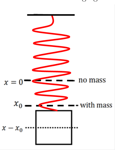
Consider the case of a vertical spring. If the spring is vertical, we have an additional force to consider: gravity. Figure 3.3 shows a spring hanging from the ceiling. Because there is a force pulling down on the spring, the spring has a different equilibrium point from the case when there is no mass hanging off it.

Figure compares the equilibrium positions for a vertical mass and spring. — Figure 3.3:Example of a vertical mass-spring system. Without the mass, the spring will have an equilibrium point at $x$ = 0. With the mass, gravity pulls down the spring until it reaches a new equilibrium point at $x = x_{0}$ , where $x_{0}< 0$ . If the mass is displaced from this new equilibrium point it will undergo simple harmonic motion.

In this case, gravity stretches the spring downward, but the spring also pulls upward to counteract gravity. At some point, the spring force will balance gravity, and the system is in a new equilibrium. To find the new equilibrium position $x_{0}$ and the equation of motion, we go back to Newton’s second law.

\sum F = ma

(10)

$F_{g}+ F_{s}= ma =\Rightarrow \sum F$ is gravity $(F_{g})$ and the spring force $(F_{s})$ $ma = -kx - mg =\Rightarrow F_{g}= -mg$ and $F_{s}= -kx$ by definition $(+\hat{x}$ is up)

If the system is static, it is in equilibrium. Here, $ma$ = 0 and $-kx - mg$ = 0, which means that the new equilibrium position is $x_{0}= - \frac{mg}{k}$ . Note that $x_{0}$ is negative because we defined $x$ = 0 to be at the original equilibrium point when there is no mass on the spring and we defined $x$ as positive pointing up.

For any other position, $x$ , the system will feel a net force and $a \not =$ 0:

ma = -kx - mg

(11)

\begin{aligned} m\frac{\mathrm{d}^{2}x}{\mathrm{d}t^{2}}&=-kx+kx_{0} \\ 0&=\frac{\mathrm{d}^{2}x}{\mathrm{d}t^{2}}+\frac{k}{m}x-\frac{k}{m}x_{0} \end{aligned}

(12)

Here we used $x_{0}=-\frac{mg}{k}$ , so $-mg=kx_{0}$ .

So we have an additional (constant) term in our differential equation of motion. Nevertheless, we can still solve this second order differential equation. The trick here is that,

\frac{\mathrm{d}^{2}}{\mathrm{d}t^{2}} (x - x_{0}) = \frac{\mathrm{d}^{2}x}{\mathrm{d}t^{2}}

(13)

if $x_{0}$ is a constant. The reason is that the derivative of a constant is always zero. So the constant does not factor into the differential at all. That means that the solution to this differential equation of motion is just what we had before, but with an offset. For example, substitute $X = x - x_{0}$ . Doing this gives us:

\begin{aligned} \frac{\mathrm{d}^{2}X}{\mathrm{d}t^{2}} &= \frac{\mathrm{d}^{2}x}{\mathrm{d}t^{2}} =\Rightarrow \mathrm{where} x_{0}\mathrm{is} \mathrm{a} \mathrm{constant} \\ \frac{\mathrm{d}^{2}X}{\mathrm{d}t^{2}} &= - \frac{k}{m} X =\Rightarrow \frac{\mathrm{d}^{2}x}{\mathrm{d}t^{2}} = - \frac{k}{m} (x - x_{0}) = - \frac{k}{m} X \\ X &= A\cos (\omega _{0}t + \varphi) \end{aligned}

(14)

which is the solution for a generic simple harmonic oscillator. But since $X = x - x_{0}$ , the equation for vertical displacement $x$ is then $x - x_{0}= A\cos (\omega _{0}t + \varphi)$ , where $x_{0}$ is our new equilibrium position. The equation of motion is,

x = A\cos (\omega _{0}t + \varphi) + x_{0}

(15)

3.3 Brief Aside on the Differential Equation of Motion¶

The Differential Equation of Motion is a convenient tool to solve cases of simple harmonic motion. If you can put your physics into this format,

0 = \frac{\mathrm{d}^{2}x}{\mathrm{d}t^{2}} + Cx

(16)

where $C$ is constant with time, then you can get the angular frequency, $\omega _{0}$ (and by default, the period $T$ and frequency $f)$ directly from the equation alone. In this form, where the differential has no coefficient, $\omega _{0}^{2}= C$ . Other constants do not matter (e.g., consider the vertical spring) to solving $\omega _{0}$ . Thus, you can read off the value of $\omega _{0}$ directly from the equation.

Quick Questions

After equating all forces, you obtain a differential equation of motion of the form:

A \frac{\mathrm{d}^{2}y}{\mathrm{d}t^{2}} + \frac{4R_{1}k}{R_{2}} y + M(R_{1}^{2}+ R_{2}^{2})g = 0

(17)

where all parameters are constants except $y$ . What is the angular frequency $(\omega _{0})$ of this system? Note, you do not need to solve the differential equation of motion.

A) $\displaystyle \omega_{0}=\frac{4R_{1}k}{R_{2}}$

B) $\displaystyle \omega_{0}=\sqrt{\frac{4R_{1}k}{AR_{2}}}$

C) $\displaystyle \omega_{0}=\sqrt{\frac{4R_{1}k}{R_{2}}+M(R_{1}^{2}+R_{2}^{2})g}$

D) $\displaystyle \omega_{0}=\frac{4R_{1}k}{AR_{2}}+\frac{M(R_{1}^{2}+R_{2}^{2})g}{A}$

3.4 Simple Harmonic Motion: Pendulum¶

3.4.1 Simple Pendulum¶

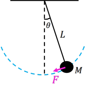
Now let’s consider a simple pendulum. A simple pendulum is a mass that hangs at the end of a string and is allowed to swing (see Figure 3.4).

Figure shows the restoring force for a simple pendulum displaced from equilibrium. — Figure 3.4:Example of a simple pendulum. The mass $m$ is in equilibrium when it is vertically downward and displaced from equilibrium when shifted an angle $\theta$ from the vertical axis. A restoring force $(F)$ moves the pendulum back to equilibrium.

A pendulum is a simple harmonic oscillator as well, because it has an equilibrium position (straight down) and a restoring force that is proportional to the displacement will seek to return the pendulum to that position.

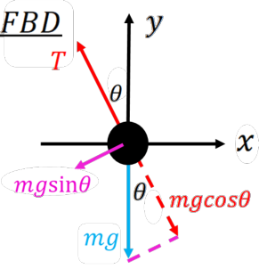
To solve for the force, let’s look at the free-body diagram of this system (Figure 3.5).

Figure shows a free-body diagram for a simple pendulum with standard Cartesian axes. — Figure 3.5:Free-body diagram of the simple pendulum from Figure 3.4. The labeled forces are tension $(T)$ in red, gravity $(mg)$ in blue, and the restoring force $(mg\sin \theta)$ in magenta. Shown in dotted-red is the component of gravity that balances tension $(mg\cos \theta)$ .

The restoring force is caused by a component of gravity that is perpendicular to the tension in the string. Because the mass-string system has an angular displacement $(\theta)$ from the equilibrium line, there is a component of gravity along the string and a component of gravity perpendicular to the string. It is the perpendicular component that is our restoring force (see magenta arrow in Figure 3.5). From trigonometry, the component parallel to the string can be written as $mg\cos \theta$ and the component perpendicular to the string is $mg\sin \theta$ . The $mg\cos \theta$ component is equal (and opposite) to the tension in the string. The $mg\sin \theta$ component is our restoring force and it will be driving our motion. So we have,

F = -mg\sin \theta

(18)

where the negative sign is present because this is a restoring force (it will act in the opposite direction to our angular displacement). Since $T$ and $mg\cos \theta$ cancel (equal and opposite forces because the string is not deforming), our net force is equal to this restoring force.

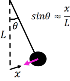
You’ll notice that this force equation does not depend on $x$ , but instead depends on the angular displacement. If we want to use $F = ma$ , we need to get the displacement in units of $x$ because $a = \ddot{x}$ . Using the small angle approximation (see Appendix B), we can write

\sin \theta = \frac{x}{L} :

(19)

Figure shows a simple pendulum and the small angle approximation. — Figure 3.6:Small angle approximation diagram for small values of $\theta$ , as this is approximately a right angle triangle where the $y-$ axis $(L)$ , and displacement $x$ meet.

The true path of the pendulum is an arc, so this assumption requires that $\theta$ isn’t too big so that there is very little difference between an arc and a straight line. See Appendix B for a review on applying small angle approximations.

So with the small angle assumption, we get

F = - \frac{mg}{L} x

(20)

where $m,g$ , and $L$ are all constants.

This equation has the exact same form as what we used for the spring $F = -kx$ , only with different constants. We can solve the equation of motion.

\sum F = ma

(21)

\begin{aligned} - \frac{mg}{L} x &= m \frac{\mathrm{d}^{2}x}{\mathrm{d}t^{2}} \\ - \frac{g}{L} x &= \frac{\mathrm{d}^{2}x}{\mathrm{d}t^{2}} \\ 0 &= \frac{\mathrm{d}^{2}x}{\mathrm{d}t^{2}} + \frac{g}{L} x \end{aligned}

(22)

Once more we have a Differential Equation of Motion that we can solve just by looking at it. This equation has the same structure as the spring and mass system. The general solution to this problem is $x(t) = A\cos (\omega _{0}t + \varphi _{1}) + B\sin (\omega _{0}t + \varphi _{2})$ , but in this case, we have a different value for the angular frequency.

\omega_{0}^{2}=\frac{g}{L}

(23)

Recall that $\omega_{0}^{2}$ equals the coefficient in front of $x$ , so

\omega_{0}=\sqrt{\frac{g}{L}}.

(24)

And the angular frequency relates to the period of motion by,

T=\frac{2\pi}{\omega_{0}}=2\pi\sqrt{\frac{L}{g}}

(25)

The period is independent of the mass of the pendulum.

3.4.2 Physical Pendulum¶

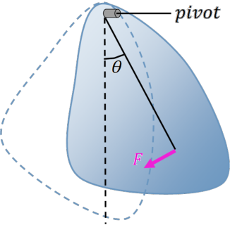
Technically, any object can be made into a pendulum if displaced from its equilibrium position and allowed to swing freely from a pivot point. We call these cases a physical pendulum. Figure 3.7 shows an example of a physical pendulum.

Figure shows an irregular object as a physical pendulum with a restoring force at the center of mass. — Figure 3.7:A physical pendulum. The irregular object has an equilibrium position as shown by the black dashed outline. When rotated out of this equilibrium position, a restoring force $F$ will seek to move it back toward equilibrium.

The solution for a physical pendulum via $F = ma$ is non-trivial, because you need to consider the acceleration of every individual particle $(F_{i}= m_{i}a_{i})$ in the system and the linear acceleration $a_{i}$ will differ throughout the system. Instead, we will revisit the physical pendulum when we discuss angular acceleration and torques in Chapter 7.

3.5 Sample Problems¶

Sample Problem 3-1

A block of mass $m$ is attached to two springs on a frictionless surface as shown in the figure below. If the block is displaced from equilibrium and set into simple harmonic motion, find the period of oscillations for the block.

Figure 3.8:Diagram of the system, with spring one having the constant $k_{1}$ and spring 2 having the constant $k_{2}$ .

Solution

Let’s first look at the free-body diagram of the system. There is the gravitational force and the normal force, which will be equal and opposite (no vertical motion). There are also restoring forces from each of the springs. If the block is displaced a distance $x$ from the equilibrium position, then the forces will be $F_{1}= -k_{1}x$ and $F_{2}= -k_{2}x$ (both springs are displaced by the same amount). The spring forces are in the same direction, because both act to move the block to equilibrium.

Continued

Figure 3.9:Free-body diagram of the block and two spring system where $F_{1}$ comes from spring 1 and $F_{2}$ comes from spring 2, and the mass has been displaced $\Delta x$ to the left.

Using Newton’s second law, the sum of all (horizontal) forces is;

\begin{aligned} \sum F&=F_{1}+F_{2}=ma \\ m\frac{\mathrm{d}^{2}x}{\mathrm{d}t^{2}}&=F_{1}+F_{2} \\ m\frac{\mathrm{d}^{2}x}{\mathrm{d}t^{2}}&=-k_{1}x-k_{2}x \\ \frac{\mathrm{d}^{2}x}{\mathrm{d}t^{2}}&=-\frac{k_{1}+k_{2}}{m}x \\ 0&=\frac{\mathrm{d}^{2}x}{\mathrm{d}t^{2}}+\frac{k_{1}+k_{2}}{m}x \end{aligned}

(26)

The vertical forces cancel because $F_g=N$ .

Again, we have a Differential Equation of Motion, and in this form, we can read off $\omega _{0}^{2}$ from the coefficient in front of the $x$ term.

\begin{aligned} \omega_{0}^{2}&=\frac{k_{1}+k_{2}}{m} \\ \omega_{0}&=\sqrt{\frac{k_{1}+k_{2}}{m}} \end{aligned}

(27)

But the question asked for the period of oscillations. For the period, we get

T = 2\pi \frac{1}{\omega _{0}}

(28)

T=2\pi\sqrt{\frac{m}{k_{1}+k_{2}}}

(29)

This is the same solution as the simple (one spring) case, but $k \rightarrow k_{1}+k_{2}$ because there are two springs working together. As a consequence of having these two springs, the period decreased compared to if there was one spring alone.

Sample Problem 3-2

A simple pendulum of mass $m$ and length $L$ is also attached to spring with spring constant $k$ as shown in the figure below. The equilibrium point for both the pendulum and spring is given by the vertical with the pivot point. If the pendulum is displaced from this equilibrium by an angle $\theta$ (like a pendulum), find the period of oscillations.

Figure 3.10:A mass $m$ forms a simple pendulum with a massless rope of length $L$ . The mass is also attached to a horizontal spring with spring constant $k$ . The equilibrium point for both the pendulum and spring is shown by the dashed vertical line (right below the pivot point).

Solution

This problem contains two simple harmonic oscillators. Let’s look at a free-body diagram for the mass. At the position of the mass, the forces are gravity on the mass, tension in the rope, and the spring force. Breaking up the gravitational force into its components along the axis of the rope and perpendicular to that axis, we get the restoring force from the pendulum as $F_{p}= F_{g}\sin \theta \approx \frac{mg}{L} x$ for small angles, $\theta$ . Note that for small angles, both the restoring forces act in the same direction.

Figure 3.11:On the left is the free-body diagram of the spring-mass system, and on the right is the component break-down of the force of gravity, $(F_{g})$ in red.

Putting these forces together, we can solve the equation of motion from the sum of all

Continued

forces:

\begin{aligned} \sum F &= F_{s}+ F_{p}= ma =\Rightarrow T \text{ and } F_{g}\cos \theta \text{ cancel, so we can ignore them} \\ ma &= -kx - \frac{mg}{L} x \\ m \frac{\mathrm{d}^{2}x}{\mathrm{d}t^{2}} &= -\bigg(k + \frac{mg}{L} \bigg)x \\ \frac{\mathrm{d}^{2}x}{\mathrm{d}t^{2}} &= -\Bigg(\frac{kL + mg}{mL} \Bigg)x \end{aligned}

(30)

0 = \frac{\mathrm{d}^{2}x}{\mathrm{d}t^{2}} + \Bigg(\frac{kL + mg}{mL} \Bigg)x

(31)

Again, we have a Differential Equation of Motion, and in this form, we can read off $\omega _{0}^{2}$ from the coefficient in front of the $x$ term.

\begin{aligned} \omega_{0}^{2}&=\frac{kL+mg}{mL} \\ \omega_{0}&=\sqrt{\frac{kL+mg}{mL}} \\ \omega_{0}&=\sqrt{\frac{k}{m}+\frac{g}{L}} \end{aligned}

(32)

The angular frequency has a term for the spring and the pendulum, which increases the value of $\omega _{0}$ compared to the value from either the spring or pendulum alone. A larger $\omega _{0}$ will decrease the period (they are inversely proportional). This means that by adding simple harmonic oscillators, the motion goes faster (shorter period).

For this $\omega _{0}$ , the period is:

T=\frac{2\pi}{\omega_{0}}=2\pi\sqrt{\frac{mL}{kL+mg}}

(33)

3.6 Aside on Damping and Driven Motion¶

The harmonic motion described above is all perfectly conserved (e.g., there is no loss of energy from friction). In practice, most oscillators undergoing harmonic motion are damped or driven. Examples of damped (energy lost) oscillations include the suspension in a vehicle (this is on purpose to limit the oscillations from bumps on the road) and tuned mass dampers in tall buildings to limit motion at high floors from earthquakes or strong winds. Examples of driven (energy gained) oscillations include pushing a child on a swing (when timed right, the child goes higher and higher) or resonances in bridges. Damped and driven motion will not be covered here.

But for fun, here are some videos that show damping motion in action. An excellent example of a tuned mass damper is the Taipei 101 building in Taiwan. Unlike most skyscrapers, the

tuned mass damper in Taipei 101 is available to be seen. Here is a nice video showing the Taipei 101 building tuned mass damper in action This video does a nice job illustrating why these dampers work.

And to also showcase driven motion, here is a video from 1940 which shows the collapse of the Tacoma Narrows bridge in the USA during a strong wind after less than four months in operation. Here is the Millennium pedestrian bridge in the UK. It did not collapse, but note how the oscillations are driven; as the bridge sways, more and more people become unbalanced at the same time and then take steps in sequence driving stronger oscillations.

3.7 Real-World Application¶

Not all oscillations are simple harmonic motion. Nevertheless, other types of periodic behaviour can be expressed with similar base mathematics even if the physics behind them is very different than a simple restoring force. These more complex cases consequently produce more complex oscillatory motions, extending the concepts of simple harmonic motion into more varied phenomena.

Seismology is the study of seismic (sound) waves that move around and through the Earth. Studying these waves can provide us information about the structure of our planet’s interior that we couldn’t otherwise constrain. The strongest seismic waves are generated by movements of tectonic plates but waves may also be caused by volcanoes, landslides, explosions, and other energetic events on and under the Earth’s surface.

Seismographs are used to record the motion of the ground due to seismic waves. Those waves travel through layers with different compositions and densities, and so are refracted and reflected. Using multiple instruments, the amount of time it takes seismic waves to travel through the Earth can be calculated and the type of material the waves are travelling through can be deduced, giving a picture of the Earth’s interior.

Since seismic waves can cause widespread damage, many agencies around the world have developed early warning systems to detect earthquakes as quickly as possible. The nationwide Earthquake Early Warning (EEW) system operated in Japan is the most advanced detection system in use, with a network of more than 4,000 seismometers.

For more information:

For some introductory science on seismic waves, you can visit the Science Learning Hub - Pokapū Akoranga Pūtaiao.

This web site contains information on earthquake warning systems in use around the world.

This interactive map uses real time data from Japan’s Earthquake Early Warning system.

3.8 Summary¶

Key Takeaways

This chapter focuses on simple harmonic motion and solving problems of simple harmonic motion using Newton’s laws. Simple harmonic motion is a periodic motion (system moves back and forth) that arises when a force has the form of

\vec{F} = -k\vec{r}

(34)

where $k$ is a constant. These types of forces are also called restoring forces, because the force itself seeks to return the system back to an equilibrium position (where the displacement is zero).

Solving Newton’s laws for simple harmonic motion yields a second-order differential equation of motion in the form of:

0 = \frac{\mathrm{d}^{2}x}{\mathrm{d}t^{2}} + Cx

(35)

where $C$ is a positive constant. This differential equation has a very well known solution of a cos (or sin) function, such as

x = A\cos (\omega _{0}t + \varphi)

(36)

A key property of simple harmonic motion is the angular frequency, $\omega _{0}$ , which can be read directly off the differential equation of motion,

\omega _{0}^{2}= C

(37)

The angular frequency is a fundamental property of the system. It depends only on the constants of the system (e.g., mass, rope length, spring constant) and it also sets the period for the periodic motion.

T = \frac{2\pi}{\omega _{0}}

(38)

Thus, if you can get a simple harmonic motion problem into its differential equation of motion, you can automatically solve for the period of motion and its angular frequency.

Important Equations

General 2nd-Order Differential:

\begin{aligned} 0 &= \frac{\mathrm{d}^{2}x}{\mathrm{d}t^{2}} + Cx \\ \mathrm{where}: \end{aligned}

(39)

C = \omega _{0}^{2}\mathrm{for} \mathrm{positive} \mathrm{constant} \mathrm{C}

(40)

\begin{aligned} \mathrm{and} \\ T &= \frac{2\pi}{\omega _{0}} \end{aligned}

(41)

2nd-Order Differential for Spring-Mass:

\frac{\mathrm{d}^{2}x}{\mathrm{d}t^{2}}=-\frac{k}{m}x, \qquad \omega_{0}=\sqrt{\frac{k}{m}}

(42)

2nd-Order Differential for Simple Pendulum:

\frac{\mathrm{d}^{2}x}{\mathrm{d}t^{2}}=-\frac{g}{L}x, \qquad \omega_{0}=\sqrt{\frac{g}{L}}

(43)

Simple Solution to 2nd-Order Differential:

x = A\cos (\omega _{0}t + \varphi _{1})

(44)

v = -\omega _{0}A\sin (\omega _{0}t + \varphi _{1})

(45)

a = -\omega _{0}^{2}x

(46)

General Solution to 2nd-Order Differential:

x = A\cos (\omega _{0}t + \varphi _{1}) + B\sin (\omega _{0}t + \varphi _{2})

(47)

v = -\omega _{0}A\sin (\omega _{0}t + \varphi _{1}) + \omega _{0}B\cos (\omega _{0}t + \varphi _{2})

(48)

a = -\omega _{0}^{2}x

(49)

3.9 Practice Problems¶

See Appendix C for answers to the practice problems.