7. Angular Momentum and Torque - Second-Year Dynamics

In this chapter, we will discuss rotational motion in the context of angular momentum and torques, and we will apply Newton’s Laws to force problems that involve rotation.

7.1 Angular Momentum¶

In Chapter 6, we introduced linear momentum, $\vec{p} = m\vec{v}$ . But objects can also move by rotation (spinning), and the momentum of a body as it undergoes rotation is called angular momentum. We define the angular momentum of a particle as:

\vec{l}_{i}= \vec{r}_{i}\times \vec{p}_{i}

(1)

where $\vec{r}_{i}$ is the position of the particle relative to the origin, and $\vec{p}_{i}$ is the momentum of that particle. The total angular momentum of a system of particles is the sum of all the particles angular momentum’s:

\vec{L} = \sum \vec{l}_{i}= \sum (\vec{r}_{i}\times \vec{p}_{i})

(2)

Note: The angular momentum is a vector quantity. The direction of the vector is given by the vector cross product of $\vec{r}$ and $\vec{p}$ (see Chapter 1.5.2 for a review of cross products).

Angular momentum is tied to circular motion. It describes any motion where there is rotation about an axis or arc-like movement. For example, an object moving in a straight line will have no angular momentum because $\vec{r}_{i}$ is parallel to $\vec{p}_{i}$ (cross product is zero). An object also has no angular momentum if it is stationary $(\vec{p}_{i}$ = 0) or it is at the origin

(\vec{r}_{i}= 0).

(3)

Like linear momentum $(\vec{p}$ ), the angular momentum in an isolated system is conserved.

7.2 Rotational Dynamics¶

7.2.1 Rotational Dynamics from Newton’s Laws¶

Another form of Newton’s laws comes from the conservation of angular momentum rather than the conservation of linear momentum. With Newton’s second law, the change in linear momentum with time is equal to the net force acting on the system.

\sum \vec{F} = \frac{\mathrm{d}\vec{p}}{\mathrm{d}t}

(4)

Now, consider the time derivative of angular momentum. For simplicity, let’s look at a single particle of mass $m_{i}$ located at a distance $r_{i}$ from the origin:

\begin{aligned} \frac{\mathrm{d}\vec{l}_{i}}{\mathrm{d}t} &= \frac{\mathrm{d}}{\mathrm{d}t} (\vec{r}_{i}\times \vec{p}_{i}) \\ &= \frac{\mathrm{d}}{\mathrm{d}t}[\vec{r}_{i}\times (m_{i}\dot{\vec{r}}_{i})] =\Rightarrow \mathrm{assume} \mathrm{mass} \mathrm{is} \mathrm{constant} \\ &= m_{i}(\dot{\vec{r}}_{i}\times \dot{\vec{r}}_{i}+ \vec{r}_{i}\times \ddot{\vec{r}}_{i}) =\Rightarrow \mathrm{apply} \mathrm{the} \mathrm{time} \mathrm{derivative} \mathrm{to} \mathrm{each} \mathrm{term} \\ &= m_{i}(0 + \vec{r}_{i}\times \ddot{\vec{r}}_{i}) =\Rightarrow \mathrm{the} \mathrm{cross} \mathrm{product} \mathrm{of} \mathrm{two} \mathrm{identical} \mathrm{vectors} \mathrm{is} \mathrm{zero} \\ &= \vec{r}_{i}\times (m_{i}\ddot{\vec{r}}_{i}) =\Rightarrow \mathrm{mass} \mathrm{is} \mathrm{a} \mathrm{constant}, \mathrm{so} \mathrm{you} \mathrm{can} \mathrm{put} \mathrm{it} \mathrm{anywhere} \\ &= \vec{r}_{i}\times \vec{F}_{i}=\Rightarrow \mathrm{recall} \mathrm{that} F = ma = m\ddot{r} \mathrm{for} \mathrm{constant} \mathrm{mass} \end{aligned}

(5)

We get that the time derivative of the angular momentum equals to the cross product of $\vec{r}$ and $\vec{F}$ . This cross product is also known as the torque, $\vec{\tau}$ .

\vec{\tau}_{i}= \vec{r}_{i}\times \vec{F}_{i}

(6)

Now, if we have a collection of particles, then we need to sum up all their individual contributions. This yields:

\sum\vec{\tau}_{i}= \sum \frac{\mathrm{d}\vec{l}_{i}}{\mathrm{d}t} = \frac{\mathrm{d}\vec{L}}{\mathrm{d}t}

(7)

where $\vec{L}$ is the total angular momentum of a system. Thus, we find that the net torque acting on a system is equal to the time derivative of the total angular momentum of that system. Equation 7.4 is Newton’s second law for rotation.

If you have a rigid body instead of a system of independent particles, then all the mass elements in the body will rotate together with the same angular velocity, $\omega$ , and angular acceleration, $\alpha$ (e.g., the body does not deform). The magnitude of the total angular momentum, $L$ , of a body is:

L = I\omega

(8)

where $I$ is the moment of inertia of the system of particles (see Section 7.2.2 for details).

Combining our equation for the total angular momentum (Equation 7.5) with the equation for the net torque (Equation 7.4), we get:

\sum\vec{\tau}=\frac{\mathrm{d}\vec{L}}{\mathrm{d}t} =\frac{\mathrm{d}(I\vec{\omega})}{\mathrm{d}t} =I\frac{\mathrm{d}\vec{\omega}}{\mathrm{d}t} =I\vec{\alpha},

(9)

where $I$ is constant in time because the system does not deform.

So similarly to $F = ma$ for the net force, we have $\tau = I\alpha$ for the net torque.

Torques in the Earth-Moon System

You’ve probably heard that the Moon causes tides on

Earth. The tides don’t occur right when the Moon is overhead, instead the tides are ahead of the Moon. As a consequence, the Earth’s tides bulge at an angle to the Moon. This bulge pulls on the Moon and the Moon in return pulls on the bulge (equal and opposite reactions), see figure (not to scale). Because these tiny forces are at an angle relative to the Earth-Moon radial line, they will each cause a torque. The torque on the Moon pulls the Moon ahead in its orbit slightly (the Moon gains momentum), whereas the torque on Earth drags the Earth slightly back in its spin (the Earth loses momentum). This is a case of angular momentum conservation! The net effect is very small, but the Moon is slowly moving away from us (at a rate of $\sim 40$ mm per year) and the Earth’s day is slowly increasing (by $\sim 2$ ms per century). For more information, see the Wikipedia webpage and Explaining Science’s webpage on tidal acceleration and the day on Earth.

7.2.2 Moment of Inertia¶

The moment of inertia, $I$ , is an important quantity in rotation. It represents how the mass of the system is distributed as a function of position and describes how efficiently the system can be rotated. It is defined as:

I = \sum_{i}m_{i}r_{i}^{2}

(11)

where $m_{i}$ is the mass of a tiny piece of the system and $r_{i}$ is the distance between that mass and the rotation axis (pivot point) of that system.

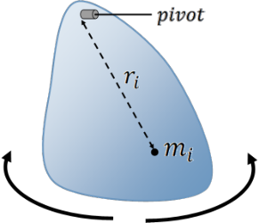
For example, Figure 7.1 shows an irregular shaped mass that is free to rotate back and forth about a pivot point toward its top. The position vector $\vec{r}_{i}$ is defined for each mass element in the object as measured from the pivot point. You must sum up all mass elements to measure the full moment of inertia for any object. Note that any mass elements at the position of the rotation axis have zero contribution to the moment of inertia because $\vec{r}_{i}$ = 0.

Figure 7.1 from the source textbook — Figure 7.1:Definition of the moment of inertia. This object will rotate about the fixed pivot point. A tiny section of mass $m_{i}$ is located a distance $r_{i}$ from that pivot point. The total moment of inertia of this system is $I = \sum(m_{i}r_{i}^{2})$ for the whole system.

Changing your moment of inertia

You can change the moment of inertia by changing the distribution of mass. For example, you could re-arrange your mass. A figure skater is an example of this. When they spin with their arms out, their moment of inertia is at its highest because they have arranged their mass (their arms) at larger radii, $I = \sum m_{i} r_{i}^{2}$ . Conversely, when they bring their arms in, their moment of inertia is smaller. Since their total angular momentum $L$ must be conserved, when the skater’s arms are out, their speed will be slower and when their arms are tucked in, their speed will be faster $(L$ = constant = $I\omega$ , so if $I$ increases, $\omega$ decreases and vice versa). See also: Video connecting rotation with the moment of inertia Video on figure skating

See Appendix A.4 for a chart of basic shapes and their moments of inertia. Most of these equations are relative to a rotation axis through the centre of mass, whereas in practice, the rotation axis could be at a different location. If you change the location of the rotation axis, you can also change the mass distribution and the moment of inertia. We can calculate the new moment of inertia using the parallel axis theorem.

Equation 7.7 gives the parallel axis theorem. Consider an object that has a moment of inertia about its centre of mass of $I_{cm}$ . If you were to pivot that object at a point $P$ that is a distance $d$ from the centre of mass, the moment of inertia about point $P$ would be.

I_{p}= I_{cm}+ Md^{2}

(12)

where $I_{p}$ is the moment of inertia about $P$ and $M$ is the total mass of the object.

7.2.3 Direction of Torque and Angular Momentum¶

Torque and angular momentum are vectors, where their directions are defined by a vector cross product, which makes finding their directions more challenging. There are several ways to get the directions. First, you can use the RHR or matrix determinant to get the direction from the definition of each vector, e.g., $\vec{\tau} = \vec{r} \times \vec{F}$ . See Chapter 1.5.2 for a review of the vector cross product.

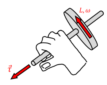
Second, you can use the RHR for rotation to connect the rotation of a system to the direction of its torque or angular momentum vectors. To apply the RHR for rotation, curl your fingers in the direction of rotation and your thumb will point in the direction of the torque vector (see also Figure 7.2). Note you can also use the RHR for rotation to get the direction of rotation if you know the direction of torque.

Cartoon demonstrating the rotational right-hand rule to determine the direction of the torque vector. — Figure 7.2:Right hand rule for connecting the direction of rotation with the direction of the torque vector.

If the torque vector points out of the page (e.g., toward you), then the system is rotating counter-clockwise. If the torque vector points into the page (away from you), then the system is rotating clockwise. When solving problems, you will want to define which of these two rotation directions (counter-clockwise versus clockwise) is positive.

7.3 The Pendulum Revisited¶

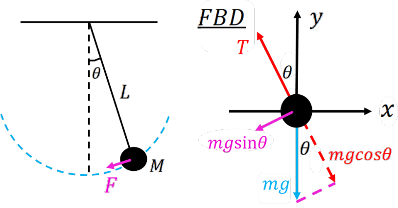
Let’s return to the pendulum program from Chapter 3.4, but this time, we’re going to solve it using torques and angular motion instead of forces and linear motion. Here is our sketch of the pendulum and the free-body diagram from before.

Figure 7.4 from the source textbook — Figure 7.4:Example of a simple pendulum. Left: The mass is in equilibrium when it is vertically downward and displaced from equilibrium when shifted an angle $\theta$ from the vertical axis. A restoring force $(F)$ moves the pendulum back to equilibrium. Right: The free-body diagram shows the labeled forces tension $(T)$ in red, gravity $(mg)$ in blue, and the restoring force $(mg\sin \theta)$ in magenta. Shown in dotted-red is the component of gravity that balances tension $(mg\cos \theta)$ .

The restoring force acting on the pendulum is given by $F = -mg\sin \theta$ . The torque acting on the pendulum is then $\vec{\tau} = \vec{r}\times \vec{F}$ . So we need to find $\vec{r}, \vec{F}$ , and the angle between them.

For our simple pendulum, $r = L$ is the distance from the pivot point to where the force is applied, which is fixed. $F$ is the restoring force, $F = -mg\sin \theta$ . By definition, the restoring force is perpendicular to the radius vector (the restoring force is given by the component of gravity that is perpendicular to the radius vector along the string, see Figure 7.4). If $\vec{r} \perp \vec{F}$ , then $\tau = rF$ . Putting this information in, we have:

\tau = |\vec{r} \times \vec{F}|

(13)

\tau = rF

(14)

\tau = -mgL\sin \theta

(15)

From Newton’s second law for rotation, the net torque is equal to:

\sum \tau = I\alpha

(16)

Since there is only one torque acting on the system (from the restoring force),

I\alpha = -mgL\sin \theta

(17)

\begin{aligned} \alpha &= - \frac{mgL}{I} \sin \theta \\ \frac{\mathrm{d}^{2}\theta}{\mathrm{d}t^{2}} &= - \frac{mgL}{I} \sin \theta \end{aligned}

(18)

This form of the differential equation of motion is difficult to solve. But, we can make it solvable by assuming that the angle formed by the pendulum and the vertical axis is small $(\theta \ll$ 1 in radian units). If $\theta$ is small, then $\sin \theta \approx \theta$ (See Appendix B) and

\frac{\mathrm{d}^{2}\theta}{\mathrm{d}t^{2}} + \frac{mgL}{I} \theta = 0

(19)

Now our equation is in the form of a simple differential equation of motion (see Chapter 3), and we know how to solve an equation in this format. The solution for $x(t)$ is a cos function with an angular frequency given by the coefficient in front of the $\theta$ term.

But wait, that isn’t the exact same solution as what we had before in Chapter 3.4. Well, there is one more step we need to do. We need to define the moment of inertia, $I$ .

For a point mass located a distance $L$ from the pivot point, the moment of inertia is just $I = mL^{2}$ . If you plug in $I = mL^{2}$ into the differential equation of motion, we get:

\frac{\mathrm{d}^{2}\theta}{\mathrm{d}t^{2}} + \frac{g}{L} \theta = 0

(20)

which is exactly the same as what we had before in Chapter 3, and it once again gives us an angular frequency of $\omega_0=\sqrt{g/L}$ .

Quick Questions

Find the angular frequency, $\omega _{0}$ , of a pendulum that consists of a rod hanging from the pivot point at one end. Assume the rod has mass $M$ and length $L$ .
You construct a pendulum by attaching a ring to a massless rod and setting it into periodic motion. Find the angular frequency, $\omega _{0}$ , of this pendulum if the rod has a length $L$ , and the ring has a mass $M$ and radius $R$ .
You have a massless rod of length $L$ to which you can attach either a solid sphere or a spherical shell. The solid sphere and spherical shells have masses and radii of (1) $M, R, (2) 2M, \frac{1}{2} R$ , or (3) $\frac{1}{2} M 2R$ . Which object will give your pendulum the shortest period and which will give you the longest period of oscillation?

7.4 The Physical Pendulum¶

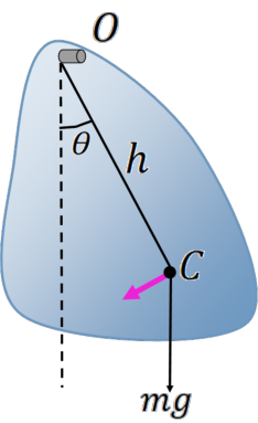
By definition, a physical pendulum is any rigid body that is free to swing about a pivot point. Figure 7.5 is an example of a physical pendulum.

Figure shows a physical pendulum of irregular shape with a pivot point near the top and the restoring force at the centre of mass toward the bottom. — Figure 7.5:A physical pendulum. The body is suspended from the point $O$ and allowed to rotate freely by an angle $\theta$ . The centre of mass of the system $C$ is located a distance $h$ from the pivot point. The total mass of the objects is $m$ . The purple arrow shows the restoring force acting on this pendulum.

Although the object has an irregular shape, the problem can be simplified by expressing the motion for the centre of mass rather than for each individual mass element of the object.

You can think of this as compressing the mass of the entire object to a single point located at the centre of mass (point C) and then determining how the restoring force acts on that compressed object. The force acting on this physical pendulum is $F = -mg\sin \theta$ at the position C. This simplification is another strength of the centre of mass.

The torque acting at the centre of mass is given by $\vec{\tau} = \vec{r}_{cm}\times F$ . The $\vec{r}_{cm}$ vector is the vector from the pivot point to the centre of mass. We know that $\vec{r}_{cm}\perp F$ , which means that our torque has a magnitude of $\tau = r_{cm}F = -mgh\sin \theta \approx -mgh\theta$ for small angles.

If this is the only torque acting on our system, Equation (7.8) becomes:

\sum \tau = I\alpha

(21)

I\alpha = -mgh\theta

(22)

0 = I\alpha + mgh\theta

(23)

0 = \frac{\mathrm{d}^{2}\theta}{\mathrm{d}t^{2}} + \frac{mgh}{I} \theta

(24)

This is the exact same equation of motion as the simple pendulum, only that the simple pendulum had the length of the rope to the mass, $L$ , and the physical pendulum has the distance between the pivot and the centre of mass $h$ .

So for a physical pendulum of any shape swinging from a pivot point that is a distance $h$ from its centre of mass, we find that the motion can be described with an angular frequency of $\omega_0=\sqrt{mgh/I}$ , where $h$ is the distance to the centre of mass and $I$ is the moment of inertia for the body. Note that for an object to be a physical pendulum, the pivot point must be located away from the centre of mass (at the centre of mass, $h=0$ ).

7.5 Example of a Physical Pendulum¶

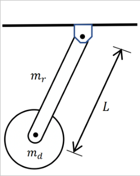
In this example, we will determine the equation of motion for a physical pendulum corresponding to a single simple harmonic oscillator.

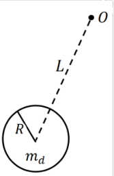
Figure shows a physical pendulum consisting of a rod and disk with the pivot point at the top of the rod and the disk at the bottom of the rod. — Figure 7.6:Diagram of the physical pendulum. This physical pendulum is constructed from a disk and rod. The disk is attached to the rod at one end and allowed to rotate freely at the other end of the rod. The disk has mass $m_{d}$ and radius $R$ . The rod has mass $m_{r}$ and length $L$ .

Solution

This system is not a simple pendulum (e.g., a point source at the end of a rope), because the rod has mass and disk has mass and dimension. So you need to consider this as a physical pendulum.

The solution for a physical pendulum is:

0 = \frac{\mathrm{d}^{2}\theta}{\mathrm{d}t^{2}} + \frac{Mgh\theta}{I}

(25)

where $h$ is the distance to the centre of mass, $M=m_r+m_d$ is the total mass of the system, and $I$ is the moment of inertia for the system (see Chapter 7.4). The solution is a cosine function with an angular frequency of $\omega_0=\sqrt{Mgh/I}$ . So the solution for the period of rotation is:

T = \frac{2\pi}{\omega _{0}}

(26)

T=2\pi\sqrt{\frac{I}{Mgh}}.

(27)

Getting the equation for the period isn’t the hard part. The trick for this problem is defining $h$ and $I$ .

Let’s start with $h$ , which is the distance from the pivot to the centre of mass of the pendulum. Since both the rod and the disk have mass, the centre of mass of the two combined is located at a mass-averaged position between the two. We will need to calculate the position of the centre of mass (see Chapter 6.4 for a definition of the centre of mass).

Fortunately, the centre of mass for each component of the pendulum is easy to calculate. The centre of mass for a uniform rod would be its midpoint and the centre of mass for a uniform disk would be its midpoint. For the rod, $r_{cm,r}= \frac{L}{2}$ (location of the midpoint of the rod from the pivot) whereas for the disk, $r_{cm,d}= L$ (location of the midpoint of the disk from the pivot). So we can treat both systems as effective point masses with all their mass at the respective centre-of-mass positions.

Thus, the centre of mass for this physical pendulum is:

h = \frac{m_{r}r_{cm,r}+ m_{d}r_{cm,d}}{m_{r}+ m_{d}}

(28)

h = \frac{m_{r}(\frac{1}{2} L) + m_{d}L}{M}

(29)

where $M = m_{r}+ m_{d}$ is the total mass of the pendulum.

Thus, we have a position for our centre of mass. Note that if our rod mass is very small (e.g., $m_{r}\rightarrow$ 0), then $M \rightarrow m_{d}$ and $r_{cm}\rightarrow L$ , or the centre of the disk. This recovers the solution for a simple pendulum.

Now let’s look at $I$ . We have two objects, a rod and a disk. To get the moment of inertia for the combined rod+disk pendulum, we can simply add the $I$ components from each object separately.

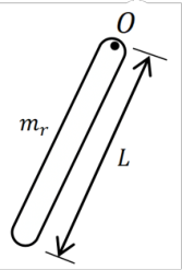
Figure shows the rod only relative to the pivot point. — Figure 7.7:Sketch of the rod with the pivot at one end.

The moment of inertia for a rod with the axis of rotation at one end is (Appendix A.4):

I_{rod}= \frac{1}{3} m_{r}L^{2}

(30)

Figure 7.8 from the source textbook — Figure 7.8:Sketch of the disk with the pivot a distance $L$ from the centre of mass.

Continued

The moment of inertia for a disk with the axis of rotation through its centre of mass is (Appendix A.4):

I_{disk}= \frac{1}{2} m_{d}R^{2}

(31)

But the pivot is not located at the centre of mass. The pivot is located a distance $L$ from the centre of mass. Therefore, we need to find $I$ for the disk about the pivot point, $O$ . Using the parallel axis theorem (Chapter 7.2.2), we have,

I_{disk,0}= \frac{1}{2} m_{d}R^{2}+ m_{d}L^{2}

(32)

Thus, the moment of inertia for the entire physical pendulum is

I = I_{rod}+ I_{disk,0}= \frac{1}{3} m_{r}L^{2}+ \frac{1}{2} m_{d}R^{2}+ m_{d}L^{2}

(33)

Taking our equations for $h$ and $I$ , we can now solve for the period:

\begin{aligned} T &=2\pi\sqrt{\frac{I}{Mgh}}\\ &=2\pi\sqrt{\frac{\left(\frac13m_r+m_d\right)L^2+\frac12m_dR^2} {gL\left(\frac12m_r+m_d\right)}}. \end{aligned}

(34)

Here the total mass $M$ cancels from the denominator.

Find the period if the disk was attached at the midpoint of the rod instead.

7.6 Example with Rolling Motion¶

In this case, we will consider a system rolling on a surface. In ideal cases, rolling motion occurs without slipping, which means that friction at the point of contact between the rolling object and the surface is sufficient to keep the system moving continuously by rolling motion. If the system is slipping, then you can get forward motion without rolling.

Sample Problem 7-2

A light cord is wrapped around the inner drum of a wheel of mass $m$ and pulled with a constant force $F$ to make the wheel roll. The wheel has a radius $R$ and the inner drum has a radius of $r$ . If the wheel rolls without slipping, what is the force of friction at the point of contact between the wheel and horizontal surface?

Figure 7.9:The applied force $(F)$ is represented by the magenta arrow, $(r)$ is the radius of the inner drum, and $(R)$ is the radius of the wheel.

Solution

First, make sure you know how this system will move. Pulling the cord in the direction shown will cause the wheel to rotate. Will it rotate clockwise or counter-clockwise? Well, let’s draw a free-body diagram to describe the forces at play in this motion and figure out how this system is going to move.

Figure 7.10:Free-body diagram of the system. The force $F$ is applied to the wheel (magenta). Also acting on the wheel are gravity (black), the normal force (blue), and friction (red). The positive $x$ and $y$ axes are shown. We have also defined the clockwise rotation direction as positive.

Overall, the wheel is moving forward in the same direction as $F$ but it is also rotating. So there are two types of motion we need to consider, translation for the forward movement and rotation for the spin of the wheel. This means we will need to consider both forms of Newton’s second law.

\sum F = ma_{cm}=\Rightarrow \mathrm{for} \mathrm{translation}

(35)

\sum \tau = I\alpha =\Rightarrow \mathrm{for} \mathrm{rotation}

(36)

Note that for the translation motion, we’re interested only in how the centre of mass is moving. That’s because the centre of mass has no rotation motion, only linear motion.

Let’s set up our coordinate system. We define $+x$ toward the right, $+y$ up, and $+\omega$ in the clockwise direction. These choices are intentional. If the linear motion is in the $+\hat{\imath}$ , then the rotation should be in the clockwise direction. While we set up the coordinate system to be most intuitive, as long as you are consistent with your defined coordinate system you will still get the correct answer.

Let’s look at $\sum F = ma_{cm}$ to start. What forces do we need to worry about for the forward motion? Both gravity and the normal force act along the $y-$ axis. These will be equal and opposite forces. The wheel does not rise above the ground nor does it sink below the ground. So we only care about $F$ and $f$ . These are opposite in direction (Figure 7.10). Based on our definition of the $+x$ axis, we have $\sum F = F - f$ .

What about $a_{cm}$ ? Keep in mind that the acceleration corresponds to the bulk forward motion of the system. If the wheel was a square box that didn’t rotate, then $a_{cm}$ would be how fast you were able to drag the box. But the magnitude of $a_{cm}$ depends on the rate of rotation because all the motion happens due to rotation (condition of rolling without slipping).

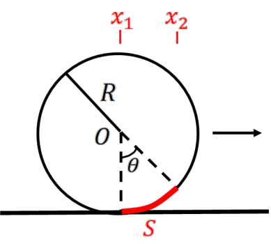
Figure 7.11 shows a schematic of our rolling wheel. The wheel is rolling forward a distance $s$ represented by the red arc. As a result of moving forward, the centre of mass has changed position from $x_{1}$ to $x_{2}$ , where $\Delta x = s$ (the translation motion is relative to the ground). That is, the system goes forward an equal distance given by the arc of the circle traveled.

Figure shows how the wheel rotates an arc length S as its center of mass moves between two points. — Figure 7.11:The rolling wheel of radius $R$ . The centre of mass is given by the origin $(O)$ and the system moves forward a distance $s$ given by the red arc.

If the system has moved a distance $s$ in time $\Delta t$ . If you have rolling without slipping, then the centre of mass motion is given by $v_{cm} = \frac{\Delta x}{\Delta t} = \frac{s}{\Delta t}$ . For very small times,

$\Delta t \rightarrow$ d $t, v_{cm}$ and $a_{cm}$ can be instead written as:

\begin{aligned} v_{cm}&= \frac{\mathrm{d}s}{\mathrm{d}t} \\ a_{cm}&= \frac{\mathrm{d}^{2}s}{\mathrm{d}t^{2}} \end{aligned}

(37)

But the arc length, $s$ can be written in terms of the angle $\theta$ and the radius $R$ . That is, $s = R\theta$ . Substituting $s = R\theta$ into our acceleration equation gives:

a_{cm}= \frac{\mathrm{d}^{2}s}{\mathrm{d}t^{2}} = \frac{\mathrm{d}^{2}R\theta}{\mathrm{d}t^{2}} = R \frac{\mathrm{d}^{2}\theta}{\mathrm{d}t^{2}} = R\alpha

(38)

The above equation gives the magnitude of $a_{cm}$ in terms of the rotation.

Assuming positive clockwise rotation, we need to check whether our $\alpha$ is also clockwise. To get the rotation direction, note that rolling happens at the point of contact where the base of the wheel meets the ground. There is only one force acting at the contact point (friction) and friction will point against the direction of motion. Using the RHR for rotation, the torque produced by the friction force is into the page and the rotation of the wheel will be clockwise. So $\alpha$ is in the clockwise direction and positive based on our definition.

Thus, combining the values of $\sum F$ and $a_{cm}$ , we get:

\sum F = ma_{cm}

(39)

F - f = mR\alpha

(40)

A key feature of this problem is the condition of rolling without slipping. This condition specifies that the rotation is entirely responsible for any forward motion such that the rotation rate can be equated to the centre of mass motion. Under this condition,

v_{cm}= \omega R

(41)

a_{cm}= \alpha R

(42)

where $\omega$ is the angular velocity and $\alpha$ is the angular acceleration. Note that the vector directions are not the same for these quantities. Only the magnitudes apply.

For a rigid object, $v_{cm}$ applies equally in magnitude and direction to the whole object (it is moving forward and doesn’t deform), whereas the motion from rotation depends on the radius and can be either forward or backwards. Consider the motion from translation and rotation at the contact point (where the wheel meets the ground). There are two velocities acting at that point, the translation velocity from $v_{cm}$ and the rotation velocity, $R\omega$ . These two velocity are equal in magnitude, but opposite in direction (at the contact point, the wheel is moving forward with $v_{cm}$ but backwards with $\omega R$ from rotation). Therefore, the contact point is instantaneously at rest. If you had rolling with slipping, then the contact point would have excess motion from translation and not be at rest.

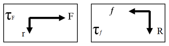
Now let’s switch to $\sum \tau = I\alpha$ . This equation describes how the wheel is going to rotate. Again, rotation and translation are two separate actions, although their magnitudes are connected due to the condition of rolling without slipping. To describe the rotation, we will want to look at how the wheel is being torqued. There are two torques acting on the wheel from $F$ and $f$ , so we want to find $\tau _{F}$ and $\tau _{f}$ .

The external force is applied at the inner radius, $r$ , whereas friction is acting at the outer radius $R$ of the wheel (where it hits the ground). Both forces are perpendicular to their radius vectors, which makes the math much easier. Figure 7.12 shows a sketch of these vectors.

Figure shows the direction of the radial vector and force vectors needed to calculate the torques produced by the applied force and the friction force. — Figure 7.12:Sketch of how the two forces produce torques. The radius vectors are defined by the origin (centre of mass location) and the forces are shown with their directions.

Since the forces are perpendicular to the radii vectors, we can simplify the torques to:

\tau _{F}= rF

(43)

\tau _{f}= Rf

(44)

But direction also matters. If you use the RHR, you will get that the external force produces a torque that is directed out of the page and the friction force produces a torque that is into the page. As a consequence, $\tau _{F}$ will produce rotation that is counterclockwise and $\tau _{f}$ will produce rotation that is clockwise. Based on our definition of positive clockwise rotation, the total torque of our system is:

\sum \tau = Rf - rF

(45)

It may seem counter intuitive to have the external force as the negative term, but this is due to our choice to define the clockwise direction as positive. Had we defined the counter-clockwise direction as positive, then we would have the external force as the positive term (but we would need a negative factor relating $a_{cm}$ and $\alpha$ ; see prior comment).

Now we have both forms of Newton’s law’s:

\sum F = ma_{cm}=\Rightarrow F - f = mR\alpha

(46)

\sum \tau = I\alpha =\Rightarrow Rf - rF = I\alpha

(47)

With two equations and two unknowns, $f$ (which we want) and $\alpha$ , we can re-arrange these equations to solve for $f$ .

\begin{aligned} \alpha &= \frac{Rf - rF}{I} (1) \\ \alpha &= \frac{F - f}{mR} (2) \end{aligned}

(48)

\frac{Rf - rF}{I} = \frac{F - f}{mR} =\Rightarrow (1) = (2)

(49)

\begin{aligned} f \bigg(\frac{R}{I} + \frac{1}{mR} \bigg) &= F \bigg(\frac{r}{I} + \frac{1}{mR} \bigg) \\ f \Bigg(\frac{mR^{2}+ I}{mRI} \Bigg) &= F \bigg(\frac{mRr + I}{mRI} \bigg) \end{aligned}

(50)

f = F \bigg(\frac{mRr + I}{mR^{2}+ I} \bigg)

(51)

To fully solve this problem, however, we need to know the moment of inertia $I$ . What is $I$ for a wheel? We will assume that the wheel consists of a thick ring with an inner

Continued

radius of $r$ and an outer radius of $R$ . In this case, the rotation axis is through the centre of the wheel, so we don’t need to apply the parallel axis theorem (Chapter 7.2.2). The moment of inertia for a thick ring with an axis through its centre is $I_{CM}= \frac{1}{2} M(r_{1}^{2}+r_{2}^{2})$ (see Appendix A.4). For our values, this gives $I = \frac{1}{2} m(r^{2}+ R^{2})$ . Adding our equation for $I$ to the problem, we get:

\begin{aligned} f &= F \Bigg(\frac{mRr + \frac{1}{2} m(r^{2}+ R^{2})}{mR^{2}+ \frac{1}{2} m(r^{2}+ R^{2})} \Bigg) \\ f &= F \frac{2Rr + r^{2}+ R^{2}}{3R^{2}+ r^{2}} \end{aligned}

(52)

Find the maximum amount of friction for the wheel if the mass is 45 kg and the coefficient of kinetic friction is $\mu _{k}= 0.15$ .
How does the maximum amount of friction compare to the friction necessary to keep the wheel rolling without slipping? Assume $r = 7.5$ cm, $R = 12.5$ cm, and $F$ = 180 N.
What force should you exert on the wheel (from b) to have it move without slipping?

7.7 Real-World Application¶

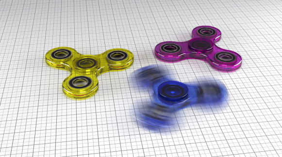
The conservation of angular momentum is a fundamental physics concept. It is sometimes referred to as Gyroscopic Motion, the tendency of a rotating object to maintain its orientation of motion. A common application you may be familiar with are fidget spinners. Fidget spinners are essentially miniature gyroscopes with a low-friction bearing to allow it to rotate longer. If you set the spinner in motion and then tilt it slowly to one side, you’ll feel it resisting the tilt, pulling back toward its original position to conserve angular momentum.

Figure shows three fidget spinners with one in motion. — Figure 7.13:Examples of fidget spinners. Image credit: Matthias Wewering from Pixabay

While the fidget spinner is an example of a simple low-weight mechanical gyroscope, there

are other types, including fluid, laser, fibre-optic, and vibrational, all working on same basic principles of rotational motion. For example, with vibrational or MEMS (Micro Electro- Mechanical System) gyroscopes, the angular velocity in the sensor produces torques on vibration elements, providing measurable displacements that can then be amplified to produce an angular velocity signal. Three sensors arranged orthogonally in a single chip provide three dimensional components and track changes in orientation. This is the type of gyroscope is used in smart phones to provide image stabilization in a camera or auto-rotation, track step counts in fitness programs, and help give accurate location and positioning with accelerometers in GPS satellites.

For more information:

For lots of detail on the physics of fidget spinners, check out this article from the International Journal for Research in Applied Science and Engineering Technology by Vandana Kaushik.

For some detail on the different types of gyroscopes, see this article from SM Lease Design.

7.8 Summary¶

Key Takeaways

This chapter introduces angular momentum and torques. Angular momentum is defined as:

\vec{L} = \vec{r} \times \vec{p}

(53)

And torque is defined as:

\vec{\tau} = \vec{r} \times \vec{F}

(54)

where both properties are vector cross products. Angular momentum and torque describe systems that are rotating. In many respects, angular momentum and torque are analogous to linear momentum and force. Newton’s second law can be written for rotation, where the net torque on a system is equal to the time derivative of the total angular momentum.

\begin{aligned} \sum \vec{\tau} &= \frac{\mathrm{d}\vec{L}}{\mathrm{d}t} \\ \sum \tau &= I\alpha \end{aligned}

(55)

A key feature of angular momentum and torques is the moment of inertia, which represents how easily a system is able to rotate.

I = \sum_{i}m_{i}r_{i}^{2}

(56)

In this chapter, we applied Newton’s second law for rotation to simple harmonic motion and rolling problems. In particular, we discussed the condition of rolling without slipping, which is a special physical case.

v_{cm}= \omega R

(57)

This condition allows you to simplify rolling problems. Rolling without slipping means that any translation (centre of mass) motion occurs due to rolling, such that forward motion can be directly connected to the rotation. If slipping occurs, then you can get forward motion independent of rotation.

Important Equations

Angular Momentum of a Particle:

\vec{l}_{i}= \vec{r}_{i}\times \vec{p}_{i}

(58)

Total Angular Momentum:

\vec{L} = \sum \vec{l}_{i}= \sum (\vec{r}_{i}\times \vec{p}_{i})

(59)

Torque:

\vec{\tau}_{i}= \vec{r}_{i}\times \vec{F}_{i}

(60)

Newton’s second law for rotation:

\begin{aligned} \sum \vec{\tau} &= \frac{\mathrm{d}\vec{L}}{\mathrm{d}t} \\ \sum \tau &= I\alpha \end{aligned}

(61)

Magnitude of Total Angular Momentum:

L = I\omega

(62)

Moment of Inertia:

I = \sum_{i}m_{i}r_{i}^{2}

(63)

Parallel Axis Theorem:

I_{P}= I_{cm}+ Md^{2}

(64)

Rolling Without Slipping Condition:

v_{cm}= \omega R

(65)

7.9 Practice Problems¶

See Appendix C for answers to the practice problems.

Practice Problem 7-1

Use the Parallel Axis Theorem to find expressions for the moments of inertia for each of the figures below. Note the location of the axis of rotation in each case.

Figure 7.14:Figure for Problem 7-1.

a) A thin disk of radius $R$ and mass $M$ rotating around an axis at its edge.

b) A rod of length $L$ and mass $M_{R}$ with a sphere of radius $R$ and mass $M_{S}$ attached to one end and the axis of rotation at the opposite end.

c) A rod of length $L$ and mass $M_{R}$ with a thin rectangular plate of mass $M_{P}$ , length $\ell$ , and width $w$ attached to one end and the axis of rotation at the opposite end.

d) A rod of length $L$ and mass $M_{R}$ with a hollow cylinder of mass $M_{C}$ , inner radius $R_{1}$ and outer radius $R_{2}$ attached to one end. The axis of rotation is through the centre of the rod.