A. Resources August 20, 2025
This Appendix contains various formulas and constants that may be used throughout this text or needed to solve problems.
A.1 Constants ¶ Quantity Symbol Value Acceleration due to gravity at Earth’s surface g g g 9.81 m s − 2 9.81\,\mathrm{m\,s^{-2}} 9.81 m s − 2 Gravitational constant G G G 6.674 × 1 0 − 11 m 3 k g − 1 s − 2 6.674\times 10^{-11}\,\mathrm{m^3\,kg^{-1}\,s^{-2}} 6.674 × 1 0 − 11 m 3 k g − 1 s − 2 Speed of light (vacuum) c c c 2.998 × 1 0 8 m s − 1 2.998\times 10^8\,\mathrm{m\,s^{-1}} 2.998 × 1 0 8 m s − 1 Speed of sound in air at 20 ∘ C 20\,{}^\circ\mathrm{C} 20 ∘ C c s c_s c s 343 m s − 1 343\,\mathrm{m\,s^{-1}} 343 m s − 1 Mass of Earth M E M_E M E 5.98 × 1 0 24 k g 5.98\times 10^{24}\,\mathrm{kg} 5.98 × 1 0 24 kg Mass of Sun M S M_S M S 1.99 × 1 0 30 k g 1.99\times 10^{30}\,\mathrm{kg} 1.99 × 1 0 30 kg Mass of Moon M M M_M M M 7.36 × 1 0 22 k g 7.36\times 10^{22}\,\mathrm{kg} 7.36 × 1 0 22 kg Mean Earth orbit (astronomical unit) r E r_E r E 1.50 × 1 0 11 m 1.50\times 10^{11}\,\mathrm{m} 1.50 × 1 0 11 m Earth radius R E R_E R E 6.37 × 1 0 6 m 6.37\times 10^6\,\mathrm{m} 6.37 × 1 0 6 m Sun radius R S R_S R S 6.96 × 1 0 8 m 6.96\times 10^8\,\mathrm{m} 6.96 × 1 0 8 m Moon radius R M R_M R M 1.74 × 1 0 6 m 1.74\times 10^6\,\mathrm{m} 1.74 × 1 0 6 m Planck constant h h h 6.63 × 1 0 − 34 J s 6.63\times 10^{-34}\,\mathrm{J\,s} 6.63 × 1 0 − 34 J s Boltzmann constant k B k_B k B 1.38 × 1 0 − 23 J K − 1 1.38\times 10^{-23}\,\mathrm{J\,K^{-1}} 1.38 × 1 0 − 23 J K − 1 Permittivity of Free Space ϵ 0 \epsilon_0 ϵ 0 8.854 × 1 0 − 12 C V − 1 m − 1 8.854\times 10^{-12}\,\mathrm{C\,V^{-1}\,m^{-1}} 8.854 × 1 0 − 12 C V − 1 m − 1 Permeability of Free Space μ 0 \mu_0 μ 0 4 π × 1 0 − 7 T m A − 1 4\pi\times 10^{-7}\,\mathrm{T\,m\,A^{-1}} 4 π × 1 0 − 7 T m A − 1 Elementary charge ∣ e ∣ \lvert e\rvert ∣ e ∣ 1.6 × 1 0 − 19 C 1.6\times 10^{-19}\,\mathrm{C} 1.6 × 1 0 − 19 C Electron mass m e m_e m e 9.11 × 1 0 − 31 k g 9.11\times 10^{-31}\,\mathrm{kg} 9.11 × 1 0 − 31 kg Proton mass m p m_p m p 1.67 × 1 0 − 27 k g 1.67\times 10^{-27}\,\mathrm{kg} 1.67 × 1 0 − 27 kg Coulomb constant k = 1 4 π ϵ 0 k=\frac{1}{4\pi\epsilon_0} k = 4 π ϵ 0 1 8.99 × 1 0 9 N m 2 C − 2 8.99\times 10^9\,\mathrm{N\,m^2\,C^{-2}} 8.99 × 1 0 9 N m 2 C − 2
Numerical values may also be presented with prefixes. For example, km corresponds to kilometer or 1000 m.
Factor Prefix Symbol Factor Prefix Symbol 10-3 milli m 103 kilo k 10-6 micro μ \mu μ 106 mega M 10-9 nano n 109 giga G 10-12 pico p 1012 tera T
A.2 Math Identities ¶ a ⃗ ⋅ b ⃗ = a b cos θ = a x b x + a y b y + a z b z \vec{a} \cdot \vec{b} = ab\cos \theta = a_{x}b_{x}+ a_{y}b_{y}+ a_{z}b_{z} a ⋅ b = ab cos θ = a x b x + a y b y + a z b z a ⃗ × b ⃗ = ( a y b z − a z b y ) ı ^ + ( a z b x − a x b z ) ȷ ^ + ( a x b y − a y b x ) k ^ , ∣ a ⃗ × b ⃗ ∣ = a b sin φ \vec{a} \times \vec{b} = (a_{y}b_{z}- a_{z}b_{y})\hat{\imath} + (a_{z}b_{x}- a_{x}b_{z})\hat{\jmath} + (a_{x}b_{y}- a_{y}b_{x})\hat{k}, |\vec{a} \times \vec{b}| = ab\sin \varphi a × b = ( a y b z − a z b y ) ^ + ( a z b x − a x b z ) ^ + ( a x b y − a y b x ) k ^ , ∣ a × b ∣ = ab sin φ ∫ d x ( x 2 + a 2 ) 3 / 2 = 1 a 2 x x 2 + a 2 , ∫ d x x 2 + a 2 = 1 a tan − 1 ( x a ) , ∫ d x a 2 − x 2 = sin − 1 ( x a ) \int \frac{\mathrm{d}x}{(x^{2}+ a^{2})^{3/2}} = \frac{1}{a^{2}} \frac{x}{\sqrt{x^{2}+ a^{2}}}, \int \frac{\mathrm{d}x}{x^{2}+ a^{2}} = \frac{1}{a} \tan ^{-1}\bigg(\frac{x}{a} \bigg), \int \frac{\mathrm{d}x}{\sqrt{a^{2}- x^{2}}} = \sin ^{-1}\bigg(\frac{x}{a} \bigg) ∫ ( x 2 + a 2 ) 3/2 d x = a 2 1 x 2 + a 2 x , ∫ x 2 + a 2 d x = a 1 tan − 1 ( a x ) , ∫ a 2 − x 2 d x = sin − 1 ( a x ) sin ( θ ± γ ) = sin θ cos γ ± cos θ sin γ , cos ( θ ± γ ) = cos θ cos γ ∓ sin θ sin γ \sin (\theta \pm \gamma) = \sin \theta \cos \gamma \pm \cos \theta \sin \gamma, \cos (\theta \pm \gamma) = \cos \theta \cos \gamma \mp \sin \theta \sin \gamma sin ( θ ± γ ) = sin θ cos γ ± cos θ sin γ , cos ( θ ± γ ) = cos θ cos γ ∓ sin θ sin γ
sin α ± sin β = 2 sin ( α ± β 2 ) cos ( α ∓ β 2 ) \sin \alpha \pm \sin \beta = 2\sin \Bigg(\frac{\alpha \pm \beta}{2} \Bigg)\cos \Bigg(\frac{\alpha \mp \beta}{2} \Bigg) sin α ± sin β = 2 sin ( 2 α ± β ) cos ( 2 α ∓ β ) cos α + cos β = 2 cos ( α + β 2 ) cos ( α − β 2 ) \cos \alpha + \cos \beta = 2\cos \Bigg(\frac{\alpha + \beta}{2} \Bigg)\cos \Bigg(\frac{\alpha - \beta}{2} \Bigg) cos α + cos β = 2 cos ( 2 α + β ) cos ( 2 α − β ) cos α − cos β = − 2 sin ( α + β 2 ) sin ( α − β 2 ) \cos \alpha - \cos \beta = -2\sin \Bigg(\frac{\alpha + \beta}{2} \Bigg)\sin \Bigg(\frac{\alpha - \beta}{2} \Bigg) cos α − cos β = − 2 sin ( 2 α + β ) sin ( 2 α − β ) ln ( a b ) = ln ( a ) + ln ( b ) , ln ( a b ) = ln ( a ) − ln ( b ) \ln (ab) = \ln (a) + \ln (b), \ln \bigg(\frac{a}{b} \bigg) = \ln (a) - \ln (b) ln ( ab ) = ln ( a ) + ln ( b ) , ln ( b a ) = ln ( a ) − ln ( b ) A.3 Common Approximations ¶ See Chapter 1.6 Appendix B
Common Taylor Series approximations for values around x ≈ 0 x \approx 0 x ≈ 0
sin x = x − x 3 3 ! + x 5 5 ! − x 7 7 ! + ⋅ ⋅ ⋅ cos x = 1 − x 2 2 ! + x 4 4 ! − x 6 6 ! + ⋅ ⋅ ⋅ e x = 1 + x + x 2 2 ! + x 3 3 ! + ⋅ ⋅ ⋅ ln ( 1 + x ) = x − x 2 2 + x 3 3 − x 4 4 + ⋅ ⋅ ⋅ 1 1 − x = 1 + x + x 2 + x 3 + ⋅ ⋅ ⋅ 1 1 + x = 1 − x + x 2 − x 3 + ⋅ ⋅ ⋅ 1 1 − x 2 = 1 + x 2 + x 4 + x 6 + ⋅ ⋅ ⋅ 1 1 + x 2 = 1 − x 2 + x 4 − x 6 + ⋅ ⋅ ⋅ 1 ( 1 − x ) 2 = 1 + 2 x + 3 x 2 + 4 x 3 + ⋅ ⋅ ⋅ 1 ( 1 + x ) 2 = 1 − 2 x + 3 x 2 − 4 x 3 + ⋅ ⋅ ⋅ \begin{aligned}
\sin x &= x - \frac{x^{3}}{3!} + \frac{x^{5}}{5!} - \frac{x^{7}}{7!} + \cdot \cdot \cdot \\
\cos x &= 1 - \frac{x^{2}}{2!} + \frac{x^{4}}{4!} - \frac{x^{6}}{6!} + \cdot \cdot \cdot \\
e^{x}&= 1 + x + \frac{x^{2}}{2!} + \frac{x^{3}}{3!} + \cdot \cdot \cdot \\
\ln (1 + x) &= x - \frac{x^{2}}{2} + \frac{x^{3}}{3} - \frac{x^{4}}{4} + \cdot \cdot \cdot \\
\frac{1}{1 - x} &= 1 + x + x^{2}+ x^{3}+ \cdot \cdot \cdot \\
\frac{1}{1 + x} &= 1 - x + x^{2}- x^{3}+ \cdot \cdot \cdot \\
\frac{1}{1 - x^{2}} &= 1 + x^{2}+ x^{4}+ x^{6}+ \cdot \cdot \cdot \\
\frac{1}{1 + x^{2}} &= 1 - x^{2}+ x^{4}- x^{6}+ \cdot \cdot \cdot \\
\frac{1}{(1 - x)^{2}} &= 1 + 2x + 3x^{2}+ 4x^{3}+ \cdot \cdot \cdot \\
\frac{1}{(1 + x)^{2}} &= 1 - 2x + 3x^{2}- 4x^{3}+ \cdot \cdot \cdot
\end{aligned} sin x cos x e x ln ( 1 + x ) 1 − x 1 1 + x 1 1 − x 2 1 1 + x 2 1 ( 1 − x ) 2 1 ( 1 + x ) 2 1 = x − 3 ! x 3 + 5 ! x 5 − 7 ! x 7 + ⋅ ⋅ ⋅ = 1 − 2 ! x 2 + 4 ! x 4 − 6 ! x 6 + ⋅ ⋅ ⋅ = 1 + x + 2 ! x 2 + 3 ! x 3 + ⋅ ⋅ ⋅ = x − 2 x 2 + 3 x 3 − 4 x 4 + ⋅ ⋅ ⋅ = 1 + x + x 2 + x 3 + ⋅ ⋅ ⋅ = 1 − x + x 2 − x 3 + ⋅ ⋅ ⋅ = 1 + x 2 + x 4 + x 6 + ⋅ ⋅ ⋅ = 1 − x 2 + x 4 − x 6 + ⋅ ⋅ ⋅ = 1 + 2 x + 3 x 2 + 4 x 3 + ⋅ ⋅ ⋅ = 1 − 2 x + 3 x 2 − 4 x 3 + ⋅ ⋅ ⋅ 1 1 − x = 1 + x 2 + 3 x 2 8 + 5 x 3 16 + ⋅ ⋅ ⋅ 1 1 + x = 1 − x 2 + 3 x 2 8 − 5 x 3 16 + ⋅ ⋅ ⋅ \begin{aligned}
\frac{1}{\sqrt{1 - x}} &= 1 + \frac{x}{2} + \frac{3x^{2}}{8} + \frac{5x^{3}}{16} + \cdot \cdot \cdot \\
\frac{1}{\sqrt{1 + x}} &= 1 - \frac{x}{2} + \frac{3x^{2}}{8} - \frac{5x^{3}}{16} + \cdot \cdot \cdot
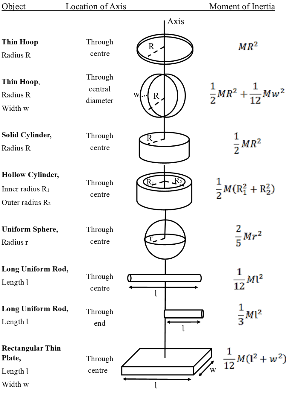
\end{aligned} 1 − x 1 1 + x 1 = 1 + 2 x + 8 3 x 2 + 16 5 x 3 + ⋅ ⋅ ⋅ = 1 − 2 x + 8 3 x 2 − 16 5 x 3 + ⋅ ⋅ ⋅ 1 1 − x 2 = 1 + x 2 2 + 3 x 4 8 + 5 x 6 16 + ⋅ ⋅ ⋅ 1 1 + x 2 = 1 − x 2 2 + 3 x 4 8 − 5 x 6 16 + ⋅ ⋅ ⋅ \frac{1}{\sqrt{1 - x^{2}}} = 1 + \frac{x^{2}}{2} + \frac{3x^{4}}{8} + \frac{5x^{6}}{16} + \cdot \cdot \cdot \frac{1}{\sqrt{1 + x^{2}}} = 1 - \frac{x^{2}}{2} + \frac{3x^{4}}{8} - \frac{5x^{6}}{16} + \cdot \cdot \cdot 1 − x 2 1 = 1 + 2 x 2 + 8 3 x 4 + 16 5 x 6 + ⋅ ⋅ ⋅ 1 + x 2 1 = 1 − 2 x 2 + 8 3 x 4 − 16 5 x 6 + ⋅ ⋅ ⋅ A.4 Moment of Inertia ¶ The Moment of Inertia, I I I Section 7.2.2
A.5 Vector Differential Operators ¶ This section gives the full coordinate transformations for the gradient, divergence, and curl in 3-D. The following is a brief explanation of those coordinate transformations.
A.5.1 General Coordinates ¶ In general, consider a 3-D coordinate system c 1 , c 2 c_{1}, c_{2} c 1 , c 2 c 3 c_{3} c 3 e ^ 1 , e ^ 2 \hat{e}_{1}, \hat{e}_{2} e ^ 1 , e ^ 2 e ^ 3 \hat{e}_{3} e ^ 3 c 1 , c 2 c_{1}, c_{2} c 1 , c 2 c 3 c_{3} c 3 x , y , z x,y,z x , y , z r , θ , φ r,\theta,\varphi r , θ , φ
In this general 3-D coordinate system, a line element would be
d s = ⟨ h 1 d c 1 , h 2 d c 2 , h 3 d c 3 ⟩ \mathrm{d}s = \langle h_{1}\mathrm{d}c_{1},h_{2}\mathrm{d}c_{2},h_{3}\mathrm{d}c_{3}\rangle d s = ⟨ h 1 d c 1 , h 2 d c 2 , h 3 d c 3 ⟩ where h 1 , h 2 h_{1}, h_{2} h 1 , h 2 h 3 h_{3} h 3
Because of these scale factors, the gradient, divergence, and curl transformations will be a bit different in each coordinate system. In the general form, these functions are:
The gradient of a function f f f
∇ ⃗ f = ( 1 h 1 ∂ f ∂ c 1 ) e ^ 1 + ( 1 h 2 ∂ f ∂ c 2 ) e ^ 2 + ( 1 h 3 ∂ f ∂ c 3 ) e ^ 3 \vec{\nabla}f = \Bigg(\frac{1}{h_{1}} \frac{\partial f}{\partial c_{1}} \Bigg)\hat{e}_{1}+ \Bigg(\frac{1}{h_{2}} \frac{\partial f}{\partial c_{2}} \Bigg)\hat{e}_{2}+ \Bigg(\frac{1}{h_{3}} \frac{\partial f}{\partial c_{3}} \Bigg)\hat{e}_{3} ∇ f = ( h 1 1 ∂ c 1 ∂ f ) e ^ 1 + ( h 2 1 ∂ c 2 ∂ f ) e ^ 2 + ( h 3 1 ∂ c 3 ∂ f ) e ^ 3 The divergence of a vector A ⃗ \vec{A} A
∇ ⃗ ⋅ A ⃗ = 1 h 1 h 2 h 3 [ ∂ ∂ c 1 ( h 2 h 3 A 1 ) + ∂ ∂ c 2 ( h 1 h 3 A 2 ) + ∂ ∂ c 3 ( h 1 h 2 A 3 ) ] \vec{\nabla} \cdot \vec{A} = \frac{1}{h_{1}h_{2}h_{3}} \Bigg[\frac{\partial}{\partial c_{1}} (h_{2}h_{3}A_{1}) + \frac{\partial}{\partial c_{2}} (h_{1}h_{3}A_{2}) + \frac{\partial}{\partial c_{3}} (h_{1}h_{2}A_{3})\Bigg] ∇ ⋅ A = h 1 h 2 h 3 1 [ ∂ c 1 ∂ ( h 2 h 3 A 1 ) + ∂ c 2 ∂ ( h 1 h 3 A 2 ) + ∂ c 3 ∂ ( h 1 h 2 A 3 ) ] and the curl of a vector A ⃗ \vec{A} A
∇ ⃗ × A ⃗ = 1 h 1 h 2 h 3 ∣ h 1 e ^ 1 h 2 e ^ 2 h 3 e ^ 3 ∂ ∂ c 1 ∂ ∂ c 2 ∂ ∂ c 3 h 1 A 1 h 2 A 2 h 3 A 3 ∣ \vec{\nabla} \times \vec{A} = \frac{1}{h_{1}h_{2}h_{3}}
\begin{vmatrix}
h_{1}\hat{e}_{1} & h_{2}\hat{e}_{2} & h_{3}\hat{e}_{3} \\
\dfrac{\partial}{\partial c_{1}} & \dfrac{\partial}{\partial c_{2}} & \dfrac{\partial}{\partial c_{3}} \\
h_{1}A_{1} & h_{2}A_{2} & h_{3}A_{3}
\end{vmatrix} ∇ × A = h 1 h 2 h 3 1 ∣ ∣ h 1 e ^ 1 ∂ c 1 ∂ h 1 A 1 h 2 e ^ 2 ∂ c 2 ∂ h 2 A 2 h 3 e ^ 3 ∂ c 3 ∂ h 3 A 3 ∣ ∣ A.5.2 Cartesian Coordinates ¶ In the Cartesian system, we have c 1 = x , c 2 = y c_{1}= x, c_{2}= y c 1 = x , c 2 = y c 3 = z c_{3}= z c 3 = z h 1 = 1 , h 2 h_{1}= 1, h_{2} h 1 = 1 , h 2 h 3 h_{3} h 3
∇ ⃗ f = ∂ f ∂ x x ^ + ∂ f ∂ y y ^ + ∂ f ∂ z z ^ \vec{\nabla}f = \frac{\partial f}{\partial x} \hat{x} + \frac{\partial f}{\partial y} \hat{y} + \frac{\partial f}{\partial z} \hat{z} ∇ f = ∂ x ∂ f x ^ + ∂ y ∂ f y ^ + ∂ z ∂ f z ^ ∇ ⃗ ⋅ A ⃗ = [ ∂ ∂ x ( A 1 ) + ∂ ∂ y ( A 2 ) + ∂ ∂ z ( A 3 ) ] \vec{\nabla} \cdot \vec{A} = \Bigg[\frac{\partial}{\partial x} (A_{1}) + \frac{\partial}{\partial y} (A_{2}) + \frac{\partial}{\partial z} (A_{3})\Bigg] ∇ ⋅ A = [ ∂ x ∂ ( A 1 ) + ∂ y ∂ ( A 2 ) + ∂ z ∂ ( A 3 ) ] ∇ ⃗ × A ⃗ = ∣ x ^ y ^ z ^ ∂ ∂ x ∂ ∂ y ∂ ∂ z A 1 A 2 A 3 ∣ \vec{\nabla} \times \vec{A} =
\begin{vmatrix}
\hat{x} & \hat{y} & \hat{z} \\
\dfrac{\partial}{\partial x} & \dfrac{\partial}{\partial y} & \dfrac{\partial}{\partial z} \\
A_{1} & A_{2} & A_{3}
\end{vmatrix} ∇ × A = ∣ ∣ x ^ ∂ x ∂ A 1 y ^ ∂ y ∂ A 2 z ^ ∂ z ∂ A 3 ∣ ∣ where x ^ \hat{x} x ^ ı ^ , y ^ \hat{\imath}, \hat{y} ^ , y ^ ȷ ^ \hat{\jmath} ^ z ^ \hat{z} z ^ k ^ \hat{k} k ^
A.5.3 Cylindrical Coordinates ¶ In cylindrical coordinates, c 1 = r , c 2 = θ c_{1}= r, c_{2}= \theta c 1 = r , c 2 = θ c 3 = z c_{3}= z c 3 = z
x = r cos φ y = r sin φ \begin{aligned}
x &= r\cos \varphi \\
y &= r\sin \varphi
\end{aligned} x y = r cos φ = r sin φ For cylindrical coordinates, h 1 = 1 , h 2 = r h_{1}= 1, h_{2}= r h 1 = 1 , h 2 = r h 3 h_{3} h 3
d V = r d r d θ d z dV = r \mathrm{d}r\mathrm{d}\theta \mathrm{d}z d V = r d r d θ d z Based on the above, we get the following for cylindrical coordinates.
∇ ⃗ f = ( ∂ f ∂ r ) r ^ + ( 1 r ∂ f ∂ θ ) θ ^ + ( ∂ f ∂ z ) z ^ \vec{\nabla}f = \Bigg(\frac{\partial f}{\partial r} \Bigg)\hat{r} + \Bigg(\frac{1}{r} \frac{\partial f}{\partial \theta} \Bigg)\hat{\theta} + \Bigg(\frac{\partial f}{\partial z} \Bigg)\hat{z} ∇ f = ( ∂ r ∂ f ) r ^ + ( r 1 ∂ θ ∂ f ) θ ^ + ( ∂ z ∂ f ) z ^ ∇ ⃗ ⋅ A ⃗ = 1 r [ ∂ ∂ r ( r A 1 ) + ∂ ∂ θ ( A 2 ) + ∂ ∂ z ( r A 3 ) ] \vec{\nabla} \cdot \vec{A} = \frac{1}{r} \Bigg[\frac{\partial}{\partial r} (rA_{1}) + \frac{\partial}{\partial \theta} (A_{2}) + \frac{\partial}{\partial z} (rA_{3})\Bigg] ∇ ⋅ A = r 1 [ ∂ r ∂ ( r A 1 ) + ∂ θ ∂ ( A 2 ) + ∂ z ∂ ( r A 3 ) ] ∇ ⃗ × A ⃗ = 1 r ∣ r ^ r θ ^ z ^ ∂ ∂ r ∂ ∂ θ ∂ ∂ z A 1 r A 2 A 3 ∣ \vec{\nabla} \times \vec{A} = \frac{1}{r}
\begin{vmatrix}
\hat{r} & r\hat{\theta} & \hat{z} \\
\dfrac{\partial}{\partial r} & \dfrac{\partial}{\partial \theta} & \dfrac{\partial}{\partial z} \\
A_{1} & rA_{2} & A_{3}
\end{vmatrix} ∇ × A = r 1 ∣ ∣ r ^ ∂ r ∂ A 1 r θ ^ ∂ θ ∂ r A 2 z ^ ∂ z ∂ A 3 ∣ ∣ A.5.4 Spherical Coordinates ¶ In spherical coordinates, c 1 = r , c 2 = θ c_{1}= r, c_{2}= \theta c 1 = r , c 2 = θ c 3 = φ c_{3}= \varphi c 3 = φ
x = r sin θ cos φ y = r sin θ sin φ z = r cos θ \begin{aligned}
x &= r\sin \theta \cos \varphi \\
y &= r\sin \theta \sin \varphi \\
z &= r\cos \theta
\end{aligned} x y z = r sin θ cos φ = r sin θ sin φ = r cos θ For spherical coordinates, h 1 = 1 , h 2 = r h_{1}= 1, h_{2}= r h 1 = 1 , h 2 = r h 3 = r sin θ h_{3}= r\sin \theta h 3 = r sin θ
d V = r 2 sin θ d r d θ d φ dV = r^{2}\sin \theta \mathrm{d}r\mathrm{d}\theta \mathrm{d}\varphi d V = r 2 sin θ d r d θ d φ Based on the above, we get the following for spherical coordinates.
∇ ⃗ f = ( ∂ f ∂ r ) r ^ + ( 1 r ∂ f ∂ θ ) θ ^ + ( 1 r sin θ ∂ f ∂ φ ) φ ^ \vec{\nabla}f = \Bigg(\frac{\partial f}{\partial r} \Bigg)\hat{r} + \Bigg(\frac{1}{r} \frac{\partial f}{\partial \theta} \Bigg)\hat{\theta} + \Bigg(\frac{1}{r\sin \theta} \frac{\partial f}{\partial \varphi} \Bigg)\hat{\varphi} ∇ f = ( ∂ r ∂ f ) r ^ + ( r 1 ∂ θ ∂ f ) θ ^ + ( r sin θ 1 ∂ φ ∂ f ) φ ^ ∇ ⃗ ⋅ A ⃗ = 1 r 2 sin θ [ ∂ ∂ r ( r 2 sin θ A 1 ) + ∂ ∂ θ ( r sin θ A 2 ) + ∂ ∂ φ ( r A 3 ) ] \vec{\nabla} \cdot \vec{A} = \frac{1}{r^{2}\sin \theta} \Bigg[\frac{\partial}{\partial r} (r^{2}\sin \theta A_{1}) + \frac{\partial}{\partial \theta} (r\sin \theta A_{2}) + \frac{\partial}{\partial \varphi} (rA_{3})\Bigg] ∇ ⋅ A = r 2 sin θ 1 [ ∂ r ∂ ( r 2 sin θ A 1 ) + ∂ θ ∂ ( r sin θ A 2 ) + ∂ φ ∂ ( r A 3 ) ] ∇ ⃗ × A ⃗ = 1 r 2 sin θ ∣ r ^ r θ ^ r sin θ φ ^ ∂ ∂ r ∂ ∂ θ ∂ ∂ φ A 1 r A 2 r sin θ A 3 ∣ \vec{\nabla} \times \vec{A} = \frac{1}{r^{2}\sin \theta}
\begin{vmatrix}
\hat{r} & r\hat{\theta} & r\sin\theta\,\hat{\varphi} \\
\dfrac{\partial}{\partial r} & \dfrac{\partial}{\partial \theta} & \dfrac{\partial}{\partial \varphi} \\
A_{1} & rA_{2} & r\sin\theta\,A_{3}
\end{vmatrix} ∇ × A = r 2 sin θ 1 ∣ ∣ r ^ ∂ r ∂ A 1 r θ ^ ∂ θ ∂ r A 2 r sin θ φ ^ ∂ φ ∂ r sin θ A 3 ∣ ∣