5. Application of Non-Inertial and Rotating Frames

In this chapter, we will use non-inertial and rotating frames of reference to solve physics problems. Please see Chapter 4 for an introduction to non-inertial and rotating frames.

5.1 Rotating versus Accelerating Frames¶

In Chapter 4, we derived the equations for acceleration and velocity in a non-inertial frame when there was only linear acceleration (Chapter 4.2) and when there was rotation (Chapter 4.4). Note that these two equations are connected.

The equation for acceleration in a rotating frame is:

\vec{a}^{\prime }= \vec{a} - \vec{\alpha} \times \vec{r}^{\prime }- 2\vec{\omega} \times \vec{v}^{\prime }- \vec{\omega} \times (\vec{\omega} \times \vec{r}^{\prime }) - \vec{A}

(1)

where the parameters with primes are in the rotating reference frame and the parameters without primes are measured in an inertial frame. See Chapter 4.5 for what each of these terms mean. If your system is not rotating, then $\vec{\alpha} = \vec{\omega} = 0$ and we recover the same equation for a linear non-inertial frame from Chapter 4.2,

\vec{a}^{\prime }= \vec{a} - \vec{A} =\Rightarrow \mathrm{for} \mathrm{no} \mathrm{rotation}

(2)

where $\vec{A}$ is the acceleration of the non-inertial frame relative to the inertial frame.

Similarly, the equation for velocity in a rotating frame is:

\vec{v}^{\prime }= \vec{v} - \vec{\omega} \times \vec{r}^{\prime }- \vec{u}

(3)

where we have added an extra term, $\vec{u}$ , to represent the velocity of the origin in the non-inertial frame relative to the inertial frame.

Finally, we defined the fictitious forces as,

m\vec{a}'=m\vec{a} \underbrace{-m\vec{\alpha}\times\vec{r}'}_{\vec{F}_{az}} \underbrace{-2m\vec{\omega}\times\vec{v}'}_{\vec{F}_{Cor}} \underbrace{-m\vec{\omega}\times(\vec{\omega}\times\vec{r}')}_{\vec{F}_{cent}} \underbrace{-m\vec{A}}_{\vec{F}_{trans}}.

(4)

where the four labeled terms are the four fictitious forces: the azimuthal force, the Coriolis force, the centrifugal force, and the translational force. Note how each of these forces are defined with negative signs because they act opposite the direction of acceleration.

In the next two sections, we will look at examples of the centrifugal force and the Coriolis force. The azimuthal force will be left for practice. See Chapter 4 for examples of the translational force.

5.2 Centrifugal Fictitious Force¶

The centrifugal force is a consequence of a rotating frame and has the form of

\vec{F}_{cent}= -m\vec{\omega} \times (\vec{\omega} \times \vec{r}^{\prime })

(5)

Note that the acceleration from the centrifugal force is $\vec{\omega}\times (\vec{\omega}\times \vec{r}^{\prime })$ and this acceleration has the same form as the centripetal acceleration associated with circular motion (see Chapter 1). If you have circular motion, $\vec{\omega} \perp \vec{r}$ and $|\vec{F}_{circ}| = m\omega ^{2}r = \frac{mv^{2}}{r}$ .

While similar in magnitude, the direction of the centrifugal force is not the same as the direction of the centripetal acceleration. The centrifugal force points radially outward for rotating frames, whereas the centripetal acceleration points radially inward. This should make intuitive sense as fictitious forces act in the opposite direction to the acceleration in the inertial frame (negative sign in the Equation (5.5).

To prove that the centrifugal force is radially outward, let’s go through an example vector cross product for uniform circular motion with its axis of rotation pointing up $(\hat{k}^{\prime })$ . Even though we have a radial dependence with our cross product, we will use Cartesian coordinates for the rotating frame $(\hat{\imath}^{\prime },\hat{\jmath}^{\prime },\hat{k}^{\prime })$ . The reason is, in our rotating frame, the radial vector will move with the non-inertial coordinate system. That is, from the perspective of a non-inertial observer rotating with the coordinate system, the radial vector does not change. So we can define our radial vector as being along the $x-$ axis $(\vec{r}^{\prime }= r\hat{\imath}^{\prime })$ for example, and as the system rotates, our radial vector will remain along the $\hat{\imath}^{\prime }$ direction (both the position and the coordinates are rotating in this non-inertial frame).

Using $\vec{\omega} = \omega \hat{k}^{\prime }$ and $\vec{r}^{\prime }= r\hat{\imath}^{\prime }$ , the centrifugal acceleration is $\vec{\omega} \times (\vec{\omega} \times \vec{r}^{\prime }) = \omega \hat{k}^{\prime }\times (\omega \hat{k}^{\prime }\times r\hat{\imath}^{\prime })$ . To solve this problem, we need to do two cross products. First, we will do the cross product

in brackets. (See Chapter 1.5.2 for review on computing the cross product).

\begin{aligned} \hat{\imath}^{\prime }\hat{\jmath}^{\prime }\hat{k}^{\prime } \\ \vec{\omega} \times \vec{r}^{\prime }&= |0 0 \omega | = \hat{\imath}^{\prime }(0 - 0) + \hat{\jmath}^{\prime }(r\omega - 0) + \hat{k}^{\prime }(0 - 0) = r\omega \hat{\jmath}^{\prime } \\ r 0 0 \end{aligned}

(6)

Then we will take our solution to that first cross product and apply that to the second cross product.

\begin{aligned} \hat{\imath}^{\prime }\hat{\jmath}^{\prime }\hat{k}^{\prime } \\ \vec{\omega} \times (\vec{\omega} \times \vec{r}^{\prime }) &= |0 0 \omega | = \hat{\imath}^{\prime }(0 - r\omega ^{2}) + \hat{\jmath}^{\prime }(0 - 0) + \hat{k}^{\prime }(0 - 0) = -r\omega ^{2}\hat{\imath}^{\prime } \\ 0 r\omega 0 \end{aligned}

(7)

So the direction of the resulting vector from $\vec{\omega} \times (\vec{\omega} \times \vec{r}^{\prime })$ is along the radial line, pointing inward toward the origin (negative value). But the centrifugal fictitious force is equal to $\vec{F}_{cent}= -m\vec{\omega} \times (\vec{\omega} \times \vec{r}^{\prime }) = mr\omega ^{2}\hat{\imath}^{\prime }$ , which means that $\vec{F}_{cent}$ is pointing radially outward (away from the origin).

friction with the table. The friction force points inward toward the center, because the rotation makes the cat want to move outward (centrifugal force).

\vec{f} = -\mu N\hat{r} = -\mu mg\hat{r}

(9)

where $N$ is the normal force. Since there is no vertical motion, $N = mg$ . The cat will start to lose balance when the acceleration from rotation equals the (static) friction force. Any additional rotation, and the cat will start to move. From Newton’s second law, we get:

\sum \vec{F} = m\vec{a}

(10)

f = -m\omega ^{2}R\hat{r}

(11)

-\mu mg\hat{r} = -m\omega ^{2}R\hat{r}

(12)

\omega=\sqrt{\frac{\mu g}{R}}.

(13)

So in the inertial frame, we can describe the cat’s motion and the condition for slipping fairly easily. What about the non-inertial frame?

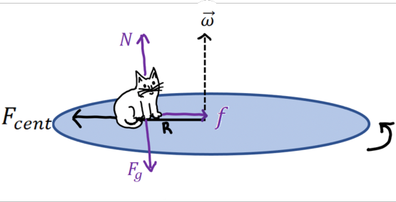
Cat’s Frame: The cat is our observer in the rotating frame, which means that the cat will experience fictitious forces. Figure 5.1 shows the free-body diagram from the cat’s perspective with vectors showing the gravitational force and the centrifugal force. Note that no other fictitious forces act on the cat, since it isn’t moving and the table is rotating at a constant rate.

Figure shows a diagram of the cat on a turntable with relevant forces labelled. — Figure 5.1:Free-body diagram for the cat on a spinning turntable. The labeled forces are the gravitational force $(F_{g})$ , the normal force $(N)$ , friction $(f)$ , and the centrifugal force $(F_{cent})$ . The three forces in purple are the forces that we would identify in an inertial frame. The centrifugal force in black is only in the cat’s frame.

Compared to the inertial frame, the cat would identify one additional force. The centrifugal force. So the sum of all forces would be:

m\vec{a}^{\prime }= \vec{F}_{I}+ \vec{F}_{cent}

(14)

where $\vec{F}_{I}$ is the total force in the inertial frame (the real forces). From the cat’s perspective, however, it isn’t moving. The cat is just sitting and the world is moving around it. So to the cat, $\vec{a}^{\prime }$ = 0.

Continued

Taking $\vec{a}^{\prime }$ = 0, we get:

0 = \vec{F}_{I}+ \vec{F}_{cent}

(15)

0 = $f + F_{cent}=\Rightarrow$ only inertial force is friction 0 = $-\mu mg + mR\omega ^{2}=\Rightarrow f$ and $F_{cent}$ act in opposite directions

\omega=\sqrt{\frac{\mu g}{R}}.

(16)

which is the same solution as the inertial frame (as expected). The difference is that we have identified the fictitious centrifugal force for the non-inertial frame.

Fictitious forces act like a modification of gravity (e.g., effective gravity) in the non-inertial frame. Depending on the problem, the effective gravity vector can be at an angle relative to the vertical. Assuming there is only the centrifugal force acting on the cat, what is the equation for the angle for the effective gravity in terms of $\omega, R$ , and $g$ ? Hint, add the $F_{g}$ and $F_{cent}$ vectors.
What is the rotation rate if the angle from the vertical is $2^{\circ}$ and $R$ = 2 m?
If the coefficient of static friction with the table is $\mu = 0.2$ , what is the maximum angular speed $(\omega _{\max})$ before the cat starts to slip?
What is the angle, relative to the vertical, of the effective gravity acting on the cat when $\omega = \omega _{\max}$ ?

Lance’s Thoughts

For a rotating frame of reference, you start with five potential fictitious forces. Most of the time, you’ll be able to eliminate at least some of them based on whether the object is moving or accelerating inside the rotating frame and whether the non-inertial frame is rotating or moving at a constant rate. Look for terms that will equal zero.

In the sample problem above, we only had centrifugal force to worry about. Since the cat, seen from inside the rotating frame, isn’t moving at all, we can eliminate the linear and Coriolis accelerations. Since the rotation is at a constant rate and the axis of rotation isn’t moving, we can eliminate the azimuthal and translational accelerations. With four out of five fictitious forces gone, this becomes a much easier problem to solve.

5.3 Coriolis Fictitious Force¶

The Coriolis force is a consequence of an object moving in a rotating frame. The force equation is:

\vec{F}_{Cor}= -2m\vec{\omega} \times \vec{v}^{\prime }

(17)

Like the centrifugal force, the Coriolis force depends on a vector cross product. So we need to look at the direction.

Let’s assume that we have a rotating system with $\vec{\omega} = \omega \hat{k}^{\prime }$ and we have a particle of mass $m$ in this system moving radially outward with a constant velocity in the rotating frame with $\vec{v}^{\prime }= v^{\prime }\hat{\imath}^{\prime }$ . As in the previous section, we will use Cartesian coordinates for simplicity, because the mass is rotating with the system such that our radial vector will remain along the $\hat{\imath}^{\prime }$ direction.

Using $\vec{\omega} = \omega \hat{k}^{\prime }$ and $\vec{v}^{\prime }= v^{\prime }\hat{\imath}^{\prime }$ , we need to solve $\vec{\omega} \times \vec{v}^{\prime }= \omega \hat{k}^{\prime }\times (v^{\prime }\hat{\imath}^{\prime })$ for the Coriolis force.

\begin{aligned} \hat{\imath}^{\prime }\hat{\jmath}^{\prime }\hat{k}^{\prime } \\ \vec{\omega} \times \vec{v}^{\prime }&= |0 0 \omega | = \hat{\imath}^{\prime }(0 - 0) + \hat{\jmath}^{\prime }(v^{\prime }\omega - 0) + \hat{k}^{\prime }(0 - 0) = v^{\prime }\omega \hat{\jmath}^{\prime } \\ v^{\prime }0 0 \end{aligned}

(18)

But the Coriolis fictitious force is equal to $\vec{F}_{Cor}= -2m\vec{\omega} \times \vec{v}^{\prime }= -2mv^{\prime }\omega \hat{\jmath}^{\prime }$ . So the Coriolis force is in the negative $\hat{\jmath}^{\prime }$ direction. You may notice this force if you’ve ever tried walking on a rotating surface (e.g., a merry-go-round). You feel off balance.

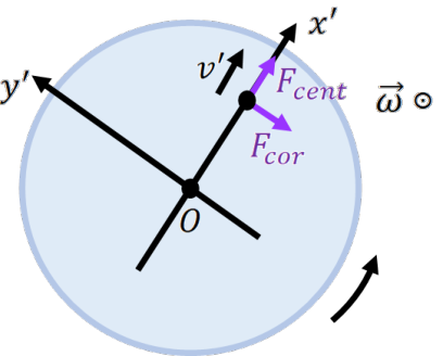
Figure 5.2 shows the fictitious forces for a particle that is moving outward with a constant velocity on a rotating reference frame. There are two fictitious forces in this case, the Coriolis force (due to motion in a rotating frame) and the centrifugal force (due to the rotating frame itself).

Figure shows the rotating x-prime y-prime coordinate plane with vectors for the fictitious forces. — Figure 5.2:Overhead view of a rotating frame with a particle of mass $m$ moving at a speed $v^{\prime }$ in the rotating frame. From the particle’s perspective, there are two fictitious forces, the centrifugal force $(F_{cent})$ and the Coriolis force $(F_{Cor})$ . Both forces only exist in the non-inertial (rotating) frame.

Sample Problem 5-2

Let’s return to the question of the cat sitting on a turntable from Sample Problem 5-1. Now, the cat starts to move radially outward at a constant speed of $v^{\prime }\hat{\imath}^{\prime }$ . At what radius will the cat start to slip?

Solution

Inertial Frame: In the inertial frame, the net force acting on the cat is still friction with the table. But due to the combination of a rotating frame and the cat is moving, friction is no longer radial (e.g., we cannot say that the cat is undergoing simple circular motion). It is much easier to solve this problem in the cat’s reference frame.

The Cat’s Frame: From the cat’s perspective, there is no acceleration because it is moving at a constant velocity. So we can simplify the equation of motion with $\vec{a}^{\prime }$ = 0. But there are two fictitious forces acting on the cat. So the force equation becomes:

m\vec{a}^{\prime }= m\vec{a} + \vec{F}_{fic}

(19)

0 = \vec{F}_{I}+ \vec{F}_{cent}+ \vec{F}_{Cor}

(20)

where $\vec{F}_{I}$ is the net force in the inertial frame. In this problem, we have $\vec{\omega} = \omega \hat{k} = \omega \hat{k}^{\prime }$ and both the radial position and the velocity vectors are along the $\hat{\imath}^{\prime }$ in the cat’s frame (these do not change from $\hat{\imath}^{\prime }$ , because the cat is rotating with the reference frame). That means we can use our previous solutions for the centrifugal and Coriolis forces (see Equations 5.6 and 5.8).

The Coriolis force is constant because the cat’s velocity and the table’s angular velocity are both constant. The Coriolis force is:

\vec{F}_{Cor}= -2m\vec{\omega} \times \vec{v}^{\prime }= -2m\omega \hat{k}^{\prime }\times (v^{\prime }\hat{\imath}^{\prime }) = -2mv^{\prime }\omega \hat{\jmath}^{\prime }

(21)

The centrifugal force is not constant, however, because the cat’s position is changing. The cat’s position can be described by $\vec{r}^{\prime }= x^{\prime }\hat{\imath}^{\prime }$ , where $\dot{x}^{\prime }= v^{\prime }$ .

\vec{F}_{cent}= -m\vec{\omega} \times (\vec{\omega} \times \vec{r}^{\prime }) = -m\omega \hat{k}^{\prime }\times (\omega \hat{k}^{\prime }\times x^{\prime }\hat{\imath}^{\prime }) = m\omega ^{2}x^{\prime }\hat{\imath}^{\prime }

(22)

Combining these equations into the force equation from the cat’s perspective, we have:

0 = \vec{F}_{I}+ \vec{F}_{cent}+ \vec{F}_{Cor}

(23)

0 = \vec{F}_{I}+ m\omega ^{2}x^{\prime }\hat{\imath}^{\prime }- 2mv^{\prime }\omega \hat{\jmath}^{\prime }

(24)

\vec{F}_{I}= 2mv^{\prime }\omega \hat{\jmath}^{\prime }- m\omega ^{2}x^{\prime }\hat{\imath}^{\prime }

(25)

Continued

We now have an equation for the net inertial force, which is only friction in this case (gravity and the normal force will cancel because the cat doesn’t leave the surface of the table). Figure 5.3 shows the direction of $\vec{F}_{I}$ in pink. Note that $\vec{F}_{I}$ is not radial because the two fictitious forces make the cat want to move in two perpendicular directions. Solving for $\vec{F}_{I}$ is very challenging in the inertial frame.

Figure 5.3:Same as Figure 5.2, but with the net force from the inertial frame included in pink. Note that $\vec{F}_{I}= -\vec{F}_{cent}- \vec{F}_{Cor}$ by definition (see above for the equation). So the net force in the inertial frame is acting at an angle.

We can use the net inertial force to get the net acceleration in the inertial frame as $\vec{a} = 2v^{\prime }\omega \hat{\jmath}^{\prime }- \omega ^{2}x^{\prime }\hat{\imath}^{\prime }$ . Note that this acceleration is not constant and it is not radial.

The condition for slipping is when the net force acting on a system has a magnitude that is equal to the static friction force, $|\vec{F}_{I}| \le f = \mu mg$ .

\mu mg = |\vec{F}_{I}|

(26)

\mu mg = |2mv^{\prime }\omega \hat{\jmath}^{\prime }- m\omega ^{2}x^{\prime }\hat{\imath}^{\prime }|

(27)

\mu mg=\sqrt{(2mv'\omega)^2+(m\omega^2x')^2}.

(28)

\mu ^{2}g^{2}= 4(v^{\prime })^{2}\omega ^{2}+ \omega ^{4}(x^{\prime })^{2}

(29)

\begin{aligned} (x^{\prime})^{2}&= \frac{\mu ^{2}g^{2}- 4(v^{\prime})^{2}\omega ^{2}}{\omega ^{4}} \\ x^{\prime}&= \dfrac{\sqrt{\mu^{2}g^{2}-4(v')^{2}\omega^{2}}}{\omega^{2}} \end{aligned}

(30)

So this is the maximum radial distance that the cat can reach before the combination of fictitious forces exceed the condition for slipping.

Consider the case where the cat walks inward toward the origin instead of outward. What is the Coriolis force in this case?
Sketch Figure 5.3 in the case where the cat walks toward the origin.

5.4 Earth as a Non-Inertial Frame¶

The Earth is rotating, which means the Earth is a non-inertial reference frame. To think about the fictitious forces acting on the Earth, it helps to think in 3-D.

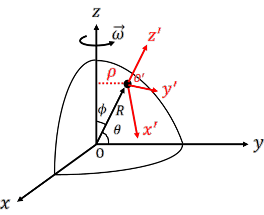
Consider Figure 5.4, which shows the position of a person on Earth’s surface. Ignoring Earth’s orbit around the Sun, we can set the inertial reference frame to the center of the planet (rotation is zero there) and we can set the non-inertial reference frame to the position of the person at the surface. Note: this example is a case where the inertial and rotating frames do not have the same origin. But the distance between them, $R$ is fixed.

Figure shows the relationship between the inertial x-y-z coordinate centered on the Earth and the rotating x-prime, y-prime, z-prime coordinate system on the Earth’s surface. — Figure 5.4:A coordinate system on Earth. The point shown is fixed to the surface of the Earth. The red coordinates show the non-inertial reference frame for an observer at this location $(O^{\prime })$ . The black coordinates show the inertial reference frame at the center of the Earth, a distance $R$ from the point. Also shown are the latitude $\theta$ , polar angle $\varphi$ , and distance to the rotation axis $\rho$ .

Our observer is located at the point shown in Figure 5.4. This person is at a latitude of $\theta$ , where the equator is located at the $x,y-$ plane of the inertial frame. We can also describe the person’s position using the polar angle $\varphi$ (also called the colatitude), where $\varphi = 90-\theta$ . In the inertial frame, these angles do not change (e.g., the latitude of a fixed point on Earth does not change), but the $x,y$ axes rotate about the $z$ axis due to Earth’s spin.

The observer on Earth’s surface has a different coordinate system that is fixed from their perspective (they don’t see the rotation). For example, here on Earth we define up and down, North and South, East and West, and those directions are fixed from our reference, even though we are on a moving surface. North is always north. Up is always up. The Earth’s motion does not change your perspective on those directions.

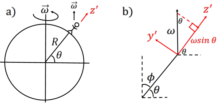
In this textbook, we will define up as $+\hat{k}^{\prime }$ , East as $+\hat{\imath}^{\prime }$ , and North as $+\hat{\jmath}^{\prime }$ for an observer in the rotating reference frame. Subsequently, down, West, and South will be the negative unit vector directions. Note that from the reference of the observer, the axis of rotation for the Earth is not along any of the unit vector axes. Figure 5.5 shows the $\hat{k}^{\prime }$ and $\hat{\jmath}^{\prime }$ components of Earth’s angular velocity vector for an observer at a latitude of $\theta$ . Note that the component of $\omega$ in the non-inertial frame depends on latitude.

From Figure 5.5, Earth’s angular velocity vector can be described as

\vec{\omega} = \omega \cos \theta \hat{\jmath}^{\prime }+ \omega \sin \theta \hat{k}^{\prime }

(31)

Thus, non-inertial motion on Earth’s surface will vary with latitude.

Figure 5.5 from the source textbook — Figure 5.5:(a) A person at a latitude of $\theta$ . The moving coordinate system has $\hat{k}^{\prime }$ normal to the surface whereas $\vec{\omega}$ is in the $\hat{k}$ direction of the inertial frame (see also, Figure 5.4). (b) Zoom in of the reference frame at a latitude of $\theta$ showing the components of $\vec{\omega}$ in the $\hat{k}^{\prime }$ and $\hat{\jmath}^{\prime }$ coordinates.

For a person on Earth’s surface moving with a constant velocity, there will be fictitious forces acting on them because they are in a non-inertial frame. Let’s look at what is at play.

\vec{a}^{\prime }= \vec{a} - \vec{\alpha} \times \vec{r}^{\prime }- 2\vec{\omega} \times \vec{v}^{\prime }- \vec{\omega} \times (\vec{\omega} \times \vec{r}^{\prime }) - \vec{A}

(32)

We can simplify this equation. We will assume that (1) the Earth’s rotation is constant, $^1$ so $\alpha = \dot{\omega}$ = 0 and (2) the origin of the non-inertial frame has no translational acceleration relative to the origin of the inertial frame $(R$ is constant, $A = \ddot{R}$ = 0). Moreover, if the person is moving with a constant velocity on Earth’s surface, $\vec{a}^{\prime }$ = 0. Taking these simplifications, the remaining fictitious forces are the centrifugal and the Coriolis forces.

$^1$ The Earth is actually slowing down in rotation due to torques with the Moon, but the change is very small and can be considered negligible.

0 = \vec{a} - 2\vec{\omega} \times \vec{v}^{\prime }- \vec{\omega} \times (\vec{\omega} \times \vec{r}^{\prime })

(33)

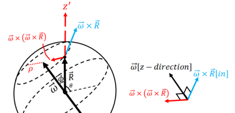
Let’s start with the centrifugal force, $F_{cent}= -m\vec{\omega} \times (\vec{\omega} \times \vec{r}^{\prime })$ .

Figure 5.6 shows the breakdown of the vector directions from the two cross products. Since $\vec{\omega}$ is not along the $\hat{k}^{\prime }$ axis and it is not perpendicular to $\vec{R}$ , getting the direction is not intuitive. You can use the right hand rule (see Chapter 1.5.2), to estimate the direction, where $\vec{\omega}\times \vec{R}$ points mostly into the page, and $\vec{\omega}\times (\vec{\omega}\times \vec{R}$ ) points mostly toward the Earth’s axis of rotation. Thus, we should expect the centrifugal force to mostly point away from the axis of rotation.

The total magnitude of the centrifugal force should therefore be given by

|\vec{F}_{cen}| = m\omega ^{2}R\sin \varphi = m\omega ^{2}R\cos \theta

(34)

where $\varphi$ is the angle between the axis of rotation and the radius vectors (see Figure 5.6). Note that $\sin \varphi = \cos \theta$ , and that the $\sin \varphi$ term only comes from the first cross product,

(\vec{\omega} \times \vec{r}^{\prime }).

(35)

As for the direction, the centrifugal force should be along an axis that is perpendicular to the rotation axis (e.g., $\hat{\rho}$ ). We can verify this by using the vector cross product, where the

Figure shows the vector directions for the centrifugal force for an observer on Earth’s surface. — Figure 5.6:The vector cross product solution for the centrifugal force at a position that is at a latitude of $\theta$ from the equator. The point $P$ is undergoing circular motion with a radius of $\rho$ , with $\rho = R\sin \varphi = R\cos \theta$ .

observer is located at $\vec{R}\hat{k}^{\prime }$ and the equation for Earth’s angular motion in the non-inertial frame from Equation 5.9.

\vec{\omega}\times\vec{r}'= \begin{vmatrix} \hat{\imath}'&\hat{\jmath}'&\hat{k}'\\ 0&\omega\cos\theta&\omega\sin\theta\\ 0&0&R \end{vmatrix} =R\omega\cos\theta\,\hat{\imath}'.

(36)

\begin{aligned} \vec{\omega}\times(\vec{\omega}\times\vec{r}') &=\begin{vmatrix} \hat{\imath}'&\hat{\jmath}'&\hat{k}'\\ 0&\omega\cos\theta&\omega\sin\theta\\ R\omega\cos\theta&0&0 \end{vmatrix}\\ &=\omega^2R\cos\theta\sin\theta\,\hat{\jmath}' -\omega^2R\cos^2\theta\,\hat{k}'. \end{aligned}

(37)

Thus, the centrifugal force will be:

\vec{F}_{cen}= -m\omega ^{2}R\cos \theta \sin \theta \hat{\jmath}^{\prime }+ m\omega ^{2}R\cos ^{2}\theta \hat{k}^{\prime }

(38)

which is pointing in a direction that is South and up. Looking at Figure 5.6, that direction points away from the rotation axis.

By contrast, gravity from the Earth is directed toward the center of the Earth, which will be along the $-\hat{k}^{\prime }$ direction, by definition. That means we have two vectors with different directions. The effective gravity will be the sum of these two vectors.

Taking the magnitude of $\vec{F}_{cen}$ , we have:

\begin{aligned} |\vec{F}_{cen}| &=\sqrt{(-m\omega^2R\cos\theta\sin\theta)^2+(m\omega^2R\cos^2\theta)^2}\\ &=m\omega^2R\cos\theta\sqrt{\sin^2\theta+\underbrace{\cos^2\theta}_{=1}}\\ &= m\omega ^{2}R\cos \theta \end{aligned}

(39)

which is what we expected using the right-hand rule and the simple vector cross product.

The total magnitude of the centrifugal force is quite small. The centrifugal force is largest at the equator $(\theta$ = 0). Taking $R$ = 6370 km for the Earth’s radius and $\omega = 7.27 \times 10^{-5}$ $\mathrm{s}^{-1}$ for the rotation rate, the centrifugal acceleration is 0.034 m $\mathrm{s}^{-2}$ , which is $< 1\%$ of the magnitude of acceleration from Earth’s gravitational field at the surface.

So for an observer on the surface of the Earth, we can generally ignore the centrifugal force from Earth’s rotation. It has a negligible effect. Thus, our vector equation for a person on Earth’s surface becomes:

\vec{a}^{\prime }= \vec{a} - 2\vec{\omega} \times \vec{v}^{\prime }

(40)

where the remaining motion is just from the inertial forces and the Coriolis force.

5.5 Foucault’s Pendulum¶

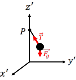
Foucault’s pendulum is a classic example of the Coriolis force in action. Consider a simple pendulum (mass hanging from an ideal string) that is also frictionless at its pivot point. Only two forces act on this pendulum, tension and gravity (see Chapter 3 and Figure 5.7).

Cartoon showing the tension and gravitational forces for a Foucault pendulum. — Figure 5.7:A Foucault pendulum of mass $m$ and length $\ell$ . The pivot point at $P$ does not move and has no friction. Two forces act in the inertial frame, tension $(\vec{T}$ ) and gravity $(\vec{F}_{g})$ . Gravity points down, tension is directed to the pivot. Note that the pendulum is moving near Earth’s surface, so we will want to use only the non-inertial coordinate system.

When set in motion, the pendulum will have a non-zero Coriolis force. Ignoring the azimuthal and centrifugal forces (negligible), we can simplify the non-inertial frame acceleration as (see previous section):

\vec{a}^{\prime }= \vec{a} - 2\vec{\omega} \times \vec{v}^{\prime }

(41)

where $a$ is the acceleration due to the net (real) forces acting on the pendulum in the inertial frame and $-2\vec{\omega} \times \vec{v}^{\prime }$ is from the Coriolis force.

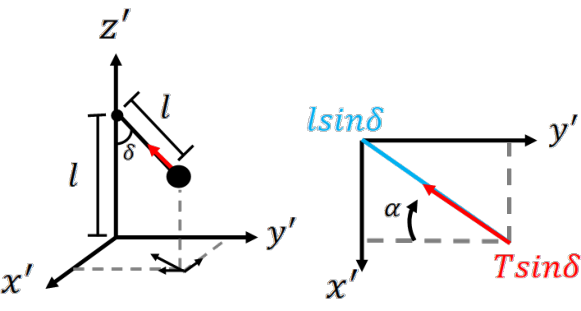
1. Finding the inertial forces: The inertial forces are gravity and tension. Gravity acts down $(-\hat{k}^{\prime }$ direction) in the non-inertial frame. So we need to convert tension to our non-inertial reference frame by finding its components along $\hat{\imath}^{\prime },\hat{\jmath}^{\prime },\hat{k}^{\prime }$ . Figure 5.8 shows the break down of the tension, $\vec{T}$ in red, into the non-inertial coordinate system.

Figure 5.8 from the source textbook — Figure 5.8:Vector diagram for tension in a pendulum relative to $\hat{\imath}^{\prime },\hat{\jmath}^{\prime },\hat{k}^{\prime }$ . Left: A 3-D view of the tension. The tension is shown by the red arrow. The pendulum makes an angle $\delta$ with respect to $\hat{k}^{\prime }$ . The black arrows at the bottom show the component of tension in the $x^{\prime },y^{\prime }$ plane and along the $x^{\prime }$ and $y^{\prime }$ axes. Right: A bird’s eye view of the $x^{\prime },y^{\prime }$ plane with the component of tension and the pendulum rope length in this plane.

The component of tension in the $x^{\prime }- y^{\prime }$ plane is $T \sin \delta$ , where $\delta$ is the angle between the pendulum and the vertical. This vector points inward toward the origin (because it is a restoring force). Figure 5.8 also shows the component of the pendulum rope length in the $x^{\prime }- y^{\prime }$ plane in blue, given by $\ell \sin \delta$ for a rope of length $\ell$ .

Using Figure 5.8 with a bit of algebra, you can get,

\vec{T} = - \frac{Tx^{\prime}}{\ell} \hat{\imath}^{\prime}- \frac{Ty^{\prime}}{\ell} \hat{\jmath}^{\prime}+ \frac{T(\ell - z^{\prime})}{\ell} \hat{k}^{\prime}

(42)

Note the negative signs for the $x^{\prime }$ and $y^{\prime }$ components. This should make sense as these would be a restoring force and restoring forces are always negative.

For the $z^{\prime }$ component, we can use the vector dot product because we know the angle between tension and $\hat{k}^{\prime }$ is $\delta$ . So $T_{z^{\prime }}= T \cos \delta$ . We can define $\cos \delta$ from the length of the rope because it is fixed. The pendulum height is given by $z^{\prime }= \ell -\ell \cos \delta$ , so we can solve for $\cos \delta = \frac{\ell -z^{\prime}}{\ell}$ . For small angles, $z^{\prime }\approx 0$ so $T_{z^{\prime }}\approx T$ .

For the $x^{\prime }$ and $y^{\prime }$ components, we use the projection of $T$ into the $x^{\prime }- y^{\prime }$ plane. The right panel of Figure 5.8 shows this projection. The $x^{\prime }-$ component is given by $T_{x^{\prime }}= T \sin \delta \sin \alpha$ , where $\sin \alpha = \frac{x^{\prime}}{\ell \sin \delta}$ , so $T_{x^{\prime }}$ simplifies to $T_{x^{\prime}}= \frac{Tx^{\prime}}{\ell}$ . Similar arguments can be made for $T_{y^{\prime }}$ .

2. Finding the non-inertial forces: For our pendulum, the only non-inertial force we

need to consider is the Coriolis force (the centrifugal force is negligible). In Section 5.3 we found the Coriolis force for a velocity in 1-D. The Foucault pendulum, however, moves in $\hat{\imath}^{\prime },\hat{\jmath}^{\prime },\hat{k}^{\prime }$ . If we assume small angles, then $z^{\prime }\ll \ell$ and any motion in the vertical direction $(\hat{k}^{\prime })$ will be negligible and we can approximate the velocity by $\vec{v}^{\prime }= \dot{x}^{\prime }\hat{\imath}^{\prime }+ \dot{y}^{\prime }\hat{\jmath}^{\prime }$ .

Using $\vec{\omega}$ from Equation 5.9 and $\vec{v}^{\prime }= \dot{x}^{\prime }\hat{\imath}^{\prime }+ \dot{y}^{\prime }\hat{\jmath}^{\prime }$ , we can solve for the Coriolis force.

\begin{aligned} \hat{\imath}^{\prime }\hat{\jmath}^{\prime }\hat{k}^{\prime } \\ \vec{\omega} \times \vec{v}^{\prime }&= |0 \omega \cos \theta \omega \sin \theta | = (-\dot{y}^{\prime }\omega \sin \theta)\hat{\imath}^{\prime }+ (\dot{x}^{\prime }\omega \sin \theta)\hat{\jmath}^{\prime }+ (-\dot{x}^{\prime }\omega \cos \theta)\hat{k}^{\prime } \\ \dot{x}^{\prime }\dot{y}^{\prime }0 \end{aligned}

(43)

The solution to the Coriolis force is then:

\vec{F}_{Cor,x^{\prime }}= 2m\dot{y}^{\prime }\omega \sin \theta

(44)

\vec{F}_{Cor,y^{\prime }}= -2m\dot{x}^{\prime }\omega \sin \theta

(45)

for the $x^{\prime }$ and $y^{\prime }$ axes, respectively. Again, we’re going to ignore the $\hat{k}^{\prime }$ component and focus on the deflection in $\hat{\imath}^{\prime }$ and $\hat{\jmath}^{\prime }$ .

3. Finding the acceleration We have descriptions for gravity, tension, and the Coriolis force in our non-inertial reference frame. We can now solve for the acceleration. For simplicity, we will do this for the $x^{\prime }$ and $y^{\prime }$ components separately. Since we are assuming negligible motion in $z^{\prime }$ , we can ignore all forces (inertial or fictitious) in the $z^{\prime }$ direction. The remaining forces in $x^{\prime }$ and $y^{\prime }$ are the inertial tension force and the fictitious Coriolis force.

\begin{aligned} m\ddot{x}^{\prime}&= - \frac{Tx^{\prime}}{l} + 2m\omega \sin \theta \dot{y}^{\prime} \\ m\ddot{y}^{\prime}&= - \frac{Ty^{\prime}}{l} - 2m\omega \sin \theta \dot{x}^{\prime} \end{aligned}

(46)

where $\theta$ is the latitude of the observer. if we assume that the angle of displacement is small, then $T \approx mg$ . So we can simplify the above as:

\begin{aligned} \ddot{x}^{\prime}&= - \frac{g}{l} x^{\prime}+ (2\omega \sin \theta)\dot{y}^{\prime} \\ \ddot{y}^{\prime}&= - \frac{g}{l} y^{\prime}- (2\omega \sin \theta)\dot{x}^{\prime} \end{aligned}

(47)

The above equations are differential equations of motion. Note that for a given observer on Earth, $\omega$ and $\theta$ are constant. The first term should look familiar. This is the solution for a simple pendulum that is displaced by a small angle from equilibrium. If $\omega$ = 0, then we recover the differential equation of motion for an ordinary pendulum in an inertial frame.

The second term comes from the Coriolis force and describe a deflection in the pendulum’s swing. This deflection always acts perpendicular to the velocity vector in the plane of motion. So instead of just oscillating back and forth in a straight line, the pendulum will slowly turn (precess) as it oscillates back and forth. The magnitude of the Coriolis force is small, but it changes the direction of the pendulum just enough that it will trace out a circle over time.

For northern latitudes $(\theta > 0)$ , the pendulum will rotate clockwise due to the Coriolis force, and for southern latitudes $(\theta < 0)$ , the pendulum will rotate counter-clockwise due to the Coriolis force. At the equator, $\theta$ = 0, and there is no deflection in the $x^{\prime }$ and $y^{\prime }$ plane. So a Foucault pendulum at the equator is just an ordinary pendulum that oscillates back and forth.

The time it takes the pendulum to complete one full circle depends on the latitude. The period for one full circle due to the Coriolis force is given by:

t_{F}= \frac{2\pi}{\omega \sin \theta} = \frac{24h}{\sin \theta}

(48)

So the Foucault pendulum offers a direct way to measure your latitude. At the North and South pole, this period is exactly 24 hours (the length of 1 day). You can say that the Earth is rotating below the pendulum as it oscillates in place due to the Coriolis force. As you approach the equator, the period gets longer. The experiment of Foucault’s pendulum was monumental for showing Earth’s rotation and that the Earth is a non-inertial frame.

5.6 Real-World Application¶

Although forces like the centrifugal force and Coriolis force are fictitious, we can see the effects of rotating references frames on objects and ourselves. A centrifuge is a device that rotates an object around a fixed axis very quickly. In laboratories, these high rotation speeds are used to separate out different substances into layers by their densities allowing pristine samples to be collected. The effective force can be hundreds or thousands of times that of a standard Earth gravity.

Rotating rides at amusement parks operate at lower speeds than centrifuges, but those on the rides feel similar effects. When on one of these rides, you would feel your body move

outward, often against the wall. Space agencies also use systems like centrifuges for highgravity simulation during astronaut training. Astronauts leaving or returning to Earth feel changes in effective gravity that can affect the blood flow to their heads and make them pass out. With training, the astronauts can simulate those conditions and learn to function.

Courtesy of the ESA astronaut Andreas Mogensen, this video shows the view from outside and inside a training centrifuge in operation.

Fisher Scientific provides a primer on centrifuge theory.

5.7 Summary¶

Key Takeaways

This chapter applies the basic concepts of non-inertial frames from Chapter 4 to more complex problems. In particular, this chapter expands on the Coriolis and centrifugal fictitious forces in rotating frames. The general equation for the fictitious forces are,

m\vec{a}'=m\vec{a} \underbrace{-m\vec{\alpha}\times\vec{r}'}_{\vec{F}_{az}} \underbrace{-2m\vec{\omega}\times\vec{v}'}_{\vec{F}_{Cor}} \underbrace{-m\vec{\omega}\times(\vec{\omega}\times\vec{r}')}_{\vec{F}_{cent}} \underbrace{-m\vec{A}}_{\vec{F}_{trans}}.

(49)

This chapter also introduces the Earth to be a non-inertial frame. To first order, the physics problems from Chapter 2 and 3 assume that the Earth is an inertial frame of reference. This approximation is generally fine, as the fictitious forces do not greatly affect these types of physics problems. Try the practice problems below to see the magnitude of some of these forces.

But for some types of high-precision physics, such as weather patterns, satellite orbits, and Foucault pendulums, you need to take into account the fictitious forces that arise from a non-inertial Earth-bound reference frame. This chapter goes through a few examples, highlighting how to breakdown and simplify such problems.

Continued

Rotation Frame Fictitious Forces:

m\vec{a}'=m\vec{a} \underbrace{-m\vec{\alpha}\times\vec{r}'}_{\vec{F}_{az}} \underbrace{-2m\vec{\omega}\times\vec{v}'}_{\vec{F}_{Cor}} \underbrace{-m\vec{\omega}\times(\vec{\omega}\times\vec{r}')}_{\vec{F}_{cent}} \underbrace{-m\vec{A}}_{\vec{F}_{trans}}.

(54)

Earth’s rotation axis for an observer on the surface:

\vec{\omega} = \omega \cos \theta \hat{\jmath}^{\prime }+ \omega \sin \theta \hat{k}^{\prime }

(55)

Centrifugal Force:

\vec{F}_{cent}= -m\vec{\omega} \times (\vec{\omega} \times \vec{r}^{\prime })

(56)

Coriolis Force:

\vec{F}_{Cor}= -2m\vec{\omega} \times \vec{v}^{\prime }

(57)

5.8 Practice Problems¶

See Appendix C for answers to the practice problems.

Practice Problem 5-9

A bead of mass $m$ sits at the end of a smooth frictionless rod of length $L$ that is rotating about one end at a rate of $\omega$ as shown in the figure below. The bead is given a little push so that it starts moving.

a) What is the magnitude and direction of the centrifugal and Coriolis forces?

b) What is the magnitude and direction of the inertial force?

c) Draw a free-body diagram for the bead in the rotating frame. What inertial force(s) are acting on the bead?

d) Use the differential equation of motion to find the equation for $x(t)$ if the initial velocity given to the bead is $\omega L$ . (Hint, you may find the following equation helpful: $\ddot{x} - C^{2}x = 0 \rightarrow x(t) = Ae^{Ct}+ Be^{-Ct}$ , where $A,B,C$ are constants)

Figure 5.10:The bead is pushed along the positive $x^{\prime }-$ axis.