4. Introduction to Non-Inertial and Rotating Frames

In this chapter, we will review inertial frames of reference and introduce non-inertial and rotating frames. A frame of reference represents your observer. Frames can be stationary, accelerating, or rotating. The physics in each of these cases will need to be treated differently.

4.1 Review of Reference Frames¶

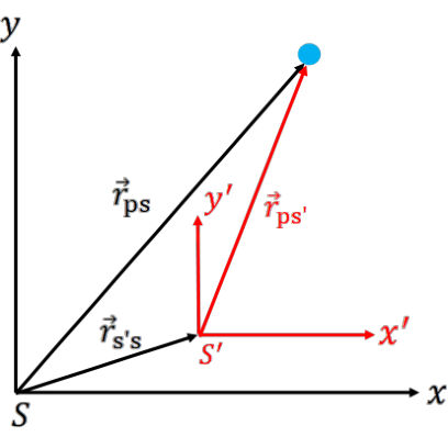
Figure 4.1 shows two reference frames with a point $P$ common to both. The black $S$ frame is stationary and the red $S^{\prime }$ frame is moving. (Imagine two observers looking at point $P$ with one observer standing still and the other is moving.) The vector from the $S$ to the point is $\vec{r}_{PS}$ and the vector from $S^{\prime }$ to the point is $\vec{r}_{PS^{\prime }}$ . The vector from $S$ to $S^{\prime }$ is $\vec{r}_{S^{\prime }S}$ . Using vector addition, you can show that $\vec{r}_{PS}= \vec{r}_{S^{\prime }S}+ \vec{r}_{PS^{\prime }}$ .

Figure compares the Cartesian coordinates for a stationary reference frame and a moving reference frame. — Figure 4.1:Sketch of two frames of reference. The black coordinate axes correspond to the inertial frame, $S$ . The red coordinate axes correspond to a moving frame, $S^{\prime }$ . A point $P$ is shown with vectors from the origin of $S$ and $S^{\prime }$ . The point is located at $\vec{r}_{PS}$ in $S$ and the point is located at $\vec{r}_{PS^{\prime }}$ in $S^{\prime }$ . The vector from $S$ to $S^{\prime }$ is $\vec{r}_{S^{\prime }S}$

Taking the time derivative and second time derivative of $\vec{r}_{PS}= \vec{r}_{S^{\prime }S}+\vec{r}_{PS^{\prime }}$ , you get velocity and acceleration.

\vec{r}_{PS}= \vec{r}_{S^{\prime }S}+ \vec{r}_{PS^{\prime }}

(1)

$\vec{v}_{PS}= \vec{v}_{S^{\prime }S}+ \vec{v}_{PS^{\prime }}=\Rightarrow$ taking the first time derivative of all terms $\vec{a}_{PS}= \vec{a}_{S^{\prime }S}+ \vec{a}_{PS^{\prime }}=\Rightarrow$ taking the second time derivative of all terms

These equations show the relative velocity and relative acceleration of P between the two frames. If $S^{\prime }$ is an inertial frame, then $S^{\prime }$ is moving with a constant velocity. For a constant velocity, $\vec{a}_{S^{\prime }S}$ = 0 and we get $\vec{a}_{PS}= \vec{a}_{PS^{\prime }}$ , the acceleration is the same in both frames. Note that the same result happens if $S^{\prime }$ is stationary.

For two different inertial frames, an observer in each frame would measure the same acceleration. There could be a difference in velocity (e.g., relative motion), but there is no difference in acceleration. As a result, there is no difference in the net forces $(\sum \vec{F} = m\vec{a})$ .

4.2 Introduction to Non-Inertial Reference Frames¶

In a non-inertial frame, the frame of reference is accelerating or rotating. Going back to our example from Section 4.1, now $\vec{a}_{S^{\prime }S}\not =$ 0 and the acceleration for point P measured in both frames will be different because,

\vec{a}_{PS}= \vec{a}_{S^{\prime }S}+ \vec{a}_{PS^{\prime }}

(2)

Let’s consider motion from the perspective of an observer in an inertial frame $(S)$ and an observer in a non-inertial frame $(S^{\prime })$ . Imagine that the two observers are sitting at the origins of each frame. They would register the motion of point $P$ relative to their frame only. So the observer in $S$ would say that the acceleration of $P$ is $\vec{a}_{PS}$ and the observer in $S^{\prime }$ would measure $\vec{a}_{PS^{\prime }}$ , where $\vec{a}_{PS}\not = \vec{a}_{PS^{\prime }}$ .

If both observers were to apply Newton’s second law, they would get: Observer in $S$ : $\sum \vec{F}_{S}= m\vec{a}_{PS}$

Observer in $S^{\prime }$ : $\sum \vec{F}_{S^{\prime }}= m\vec{a}_{PS^{\prime }}$

But $m\vec{a}_{PS}\not = m\vec{a}_{PS^{\prime }}$ , so that means $\sum \vec{F}_{S}\not = \sum \vec{F}_{S^{\prime }}$ . The two observers will measure different solutions from Newton’s laws.

But there can be only one true net force. Physics cannot change just because the reference frame has changed. It may seem like Newton’s laws have failed, but in practice, we need to apply a “correction” for the accelerating frame. This correction can be written as:

\sum \vec{F}_{S^{\prime }}= m\vec{a}_{PS^{\prime }}

(3)

\sum \vec{F}_{S^{\prime }}= m(\vec{a}_{PS}- \vec{a}_{S^{\prime }S}) =\Rightarrow \vec{a}_{PS}= \vec{a}_{S^{\prime }S}+ \vec{a}_{PS^{\prime }}

(4)

\sum \vec{F}_{S^{\prime }}= m\vec{a}_{PS}- m\vec{a}_{S^{\prime }S}

(5)

\sum \vec{F}_{S^{\prime }}= \sum \vec{F}_{S}- m\vec{a}_{S^{\prime }S}

(6)

\sum \vec{F}_{S^{\prime }}= \sum \vec{F}_{S}+ F_{fic}

(7)

where we have introduced a “new force”, $\vec{F}_{fic}$ . We call this “new force” a fictitious force or an inertial force. For the second law to match in both the inertial and non-inertial (accelerating) frame, we add in these fictitious forces to the inertial frame, where

\vec{F}_{fic}= -m\vec{a}_{S^{\prime }S}

(8)

Note that the fictitious forces do not represent actual forces. Fictitious forces do not arise from the interaction between the two frames $S$ and $S^{\prime }$ or from an interaction between the moving object and another object. Instead, they arise from the non-inertial frame having an acceleration. It is a “force” that an observer in a non-inertial frame would feel acting on them only because they are in an accelerating frame.

Cora’s Thoughts

Overall fictitious forces are forces that appear to act on an object to explain its motion. A good way to think of fictitious forces is in the context of driving a car. If you are driving a car down a straight road with cruise control on (traveling at a constant linear velocity), then you are in an inertial frame and you do not feel any forces from the motion of the car. However, when you hit a bend in the road you accelerate as you turn making the car a non-inertial frame. When the car turns left, it accelerates to the left, and you feel a “force” that pushes you to the right. That “force” is the fictitious force. It is the force felt in the opposite the direction of the acceleration, that comes from being an observer in a non-inertial frame, as you only know that you are in an accelerating frame due to feeling this fictitious force.

Figure 4.2:On the left is the inertial frame and on the right is the non-inertial frame.

Mathematically, the acceleration of the non-inertial frame causes the object to have an extra term in the force equation as measured from the perspective of someone in a true inertial frame. That extra term has the form of a force (mass times acceleration). If we need to add the fictitious force(s) to the inertial forces, then we can apply Newton’s second law to the non-inertial frame and get the same answer:

\sum \vec{F}_{S^{\prime }}= \sum \vec{F}_{S}+ \vec{F}_{fic}

(9)

m\vec{a}_{PS^{\prime }}= m\vec{a}_{PS}- m\vec{a}_{S^{\prime }S}

(10)

m\vec{a}_{PS^{\prime }}= m(\vec{a}_{S^{\prime }S}+ \vec{a}_{PS^{\prime }}) - m\vec{a}_{S^{\prime }S}=\Rightarrow \mathrm{definition} \mathrm{of} \vec{a}_{PS}

(11)

m\vec{a}_{PS^{\prime }}= m\vec{a}_{PS^{\prime }}=\Rightarrow \mathrm{left} \mathrm{side} = \mathrm{right} \mathrm{side}

(12)

So now we have matching physics in both reference frames. That is, the two observers would come to the same answer if we include a new “force”. Ultimately, an observer in a non-inertial frame must correct their net force (compared to an inertial frame) using a fictitious force.

\underbrace{\sum\vec{F}_{S'}}_{\text{non-inertial frame}} =\underbrace{\sum\vec{F}_{S}}_{\text{inertial frame}} +\underbrace{\vec{F}_{fic}}_{\text{correction}}

(13)

4.3 Example Problems with Linear Acceleration¶

Let’s put non-inertial frames into practice with a couple of examples where the acceleration is linear (no rotation).

Continued

\sum \vec{F} = m\vec{a}_{e}

(14)

T - mg = ma_{e}

(15)

T = m(a_{e}+ g)

(16)

where $a_{e}$ is the acceleration of the mass because of the elevator.

b) Elevator Frame: Now consider the observer $O^{\prime }$ in the elevator with the mass. From the perspective of this observer, the mass is stationary because both the observer and the mass are moving upwards (there is no relative motion between $O^{\prime }$ and $m)$ . So $\sum \vec{F}_{S^{\prime }}$ = 0. But we cannot say that $\sum \vec{F}_{S^{\prime }}$ is given by tension and gravity alone, because $S^{\prime }$ is in a non-inertial frame. This observer must take into account the acceleration of their own frame and include a fictitious force acting on mass.

For the moving reference frame, we need to correct the second law using the fictitious force. Taking up as positive, we have:

\sum \vec{F}_{S^{\prime }}= \sum \vec{F}_{S}+ \vec{F}_{fic}

(17)

\sum \vec{F}_{S^{\prime }}= \sum \vec{F}_{S}- ma_{e}=\Rightarrow \vec{F}_{fic}= -m\vec{a}_{S^{\prime }S}= -ma_{e}

(18)

0 = T - mg - ma_{e}=\Rightarrow m \mathrm{at} \mathrm{rest} \mathrm{in} S^{\prime }, \mathrm{so} \sum \vec{F}_{S^{\prime }}= 0

(19)

T = m(a_{e}+ g)

(20)

which is the same answer as before from the inertial frame as expected. We need our physics to match in both reference frames (or we have a problem with physics!).

Draw a free-body diagram of the mass in the inertial and non-inertial frames. What is the vector direction of the fictitious force?
Now the elevator is accelerating downward. Solve for the tension in the rope for both frames. What is the direction of the fictitious force?

Sample Problem 4-2

A truck is carrying a box of mass $m$ . When the truck decelerates at a rate of $a_{0}= 0.6g$ , the box in the rear of the truck begins to slide forward relative to an observer sitting in the truck. If the coefficient of friction between the box and the truck is $\mu = 0.4$ , what is the acceleration of the box relative to the (a) the ground and (b) the truck?

Solution

Case 1: We will first solve this problem from the perspective of an observer standing on the ground (so from the inertial frame).

Figure 4.4:Free-body diagram of the mass $m$ in the inertial frame. The forces acting on the mass are the force of friction $(f)$ in red, the normal force $(N)$ and gravity $(mg)$ .

Inertial Frame: Figure 4.4, shows the free-body diagram of the box relative to an observer in an inertial frame (e.g., an observer on the ground). If the box is moving forward $(+x$ direction), then friction is acting in the opposite direction $(-x$ direction). We also have gravity and the normal force.

All motion is horizontal. The box does not move up or down, so $\sum \vec{F}_{y}$ = 0. There are only two vertical forces, gravity and the normal force. Therefore, we can say that

N = mg.

(21)

a) To the observer on the ground (in the inertial frame), the net force acting on the box is just from friction, $\sum \vec{F}_{g}= f$ . From Newton’s second law, we have:

\sum \vec{F}_{g}= \vec{f}

(22)

ma_{b}= -\mu mg

(23)

a_{b}= -0.4g

(24)

So the acceleration of the box relative to the ground is $-0.4g$ (taking forward to be positive).

b) To get the acceleration of the box relative to the truck, $a_{b^{\prime }}$ , we use coordinate transformation. Note that the acceleration of the truck is $\vec{a}_{0}= -0.6g\hat{\imath}$ because the

truck is decelerating and we set the forward direction as the positive $x$ direction.

\vec{a}_{b^{\prime }}= \vec{a}_{b}- \vec{a}_{0}

(25)

a_{b^{\prime }}= -0.4g - (-0.6g)

(26)

a_{b^{\prime }}= 0.2g

(27)

So the acceleration of the box relative to the truck is $0.2g$ . Note that this is positive. That makes sense as the box is sliding forward relative to the observer sitting (stationary) in the truck.

Case 2: We can also solve this problem using the non-inertial frame of the truck. That is, we can solve the accelerations from the perspective of a person sitting in the truck.

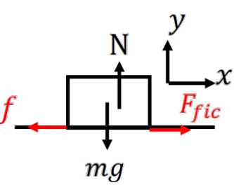
Figure shows a free body diagram for the mass in the non-inertial frame. — Figure 4.5:Free-body diagram of the mass $m$ in the non-inertial frame. The forces acting on the mass are the force of friction $(f)$ and the fictitious force $(F_{fic})$ in red, the normal force $(N)$ and gravity $(mg)$ .

Truck Frame: Figure 4.5 shows the free-body diagram of the box relative to an observer in the truck (non-inertial frame). We have the same forces as the inertial frame (friction, gravity, normal), but there is also the fictitious force.

Again, all motion is horizontal. But in the non-inertial frame of the truck, there are two horizontal forces. First, is friction given by $f = -\mu N = -\mu mg$ (negative because it acts in the $-x$ direction). Second, is the fictitious force because the truck is a non-inertial frame. Recall that fictitious forces act in the opposite direction of the acceleration of the frame relative to an inertial frame. Since the truck is decelerating $(-x$ direction) relative to the inertial frame $(a_{0}= -0.6g)$ , the fictitious force acts in the $+x$ direction.

For the non-inertial frame, we will first find $a_{b^{\prime }}$ , the acceleration of the box relative to an observer on the truck.

\sum \vec{F}_{S^{\prime }}= -\mu mg + \vec{F}_{fic}

(28)

a_{b^{\prime }}= -0.4g + 0.6g =\Rightarrow \vec{F}_{fic}= -ma_{0}\mathrm{and} a_{0}= -0.6g

(29)

a_{b^{\prime }}= 0.2g

(30)

Which is exactly what we had before from Case 1 when solving the problem from the inertial frame as expected.

4.4 Rotating Frames¶

For a review of rotational motion see Chapter 1.1.2 and for an example practice problem with rotation in an inertial frame, see Example 1-2.

4.4.1 Rotating Systems¶

In this section, we will introduce rotating non-inertial frames. We often call the Earth’s surface an inertial frame in physics, but this assumption neglects the rotation of the Earth about its axis (and the rotation of the Earth around the Sun, the rotation of the Sun around the centre of our galaxy, and the motion of our galaxy within our Local Group of galaxies...). For simple problems, we can often assume the Earth’s surface is an inertial frame. But there are physics problems that require that you take into account Earth’s own rotation.

For inertial frames, an object that is rotating with a constant angular velocity of $\vec{\omega}$ around a fixed axis has the following equations of motion.

\vec{v} = \vec{\omega} \times \vec{r}

(31)

\vec{a} = \vec{\omega} \times (\vec{\omega} \times \vec{r})

(32)

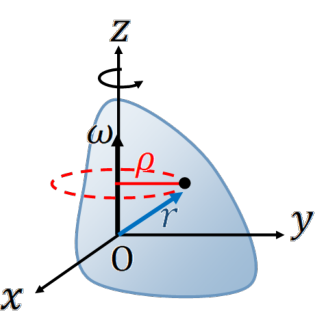
Consider an object rotating with $\omega$ in the $\hat{k}$ direction and that this axis of rotation is fixed (see Figure 4.6). A point P in this system has the vector position $\vec{r}$ . This vector position can also be described by $\vec{r} = \rho \hat{\rho}+z\hat{k}$ , where $\vec{\rho}$ is the projection of $\vec{r}$ onto the plane perpendicular to $\vec{\omega}$ (for $\vec{\omega}$ along $\hat{k}$ , this plane is the $x - y$ plane).

Figure shows an irregular object rotating around the z-axis. — Figure 4.6:An irregular object rotating in the counterclockwise direction around the $z-$ axis of an $xyz-$ axis coordinate system. The labeled point is a distance $\vec{r}$ from the origin and a distance $\rho$ from the $z-$ axis.

From this definition of $\vec{r}$ and $\vec{\rho}$ , we can show that the velocity is:

\vec{v} = \vec{\omega} \times \vec{r} = \omega r\sin \theta \hat{\theta} = \omega \rho \hat{\theta}

(33)

where $\hat{\theta}$ is an azimuthal angle between $\vec{\omega}$ and $\vec{r}$ .

Similarly, we can show that the magnitude of acceleration is:

\vec{a} = -\omega ^{2}\vec{\rho}

(34)

since $\vec{a} = \vec{\omega} \times (\vec{\omega} \times \vec{r}) = \vec{\omega} \times (\omega \rho \hat{\theta}$ ), and $\vec{\omega} \perp \hat{\theta}$ . The negative sign arises from the cross product and indicates that the acceleration is directed toward the rotation axis. See Chapter 1.5.2 for a review of vector cross products and the right-hand rule.

4.4.2 Coordinate System of a Rotating Frame: Velocity¶

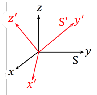
Figure 4.7 shows the coordinates for an inertial frame, $S$ , in black and a non-inertial rotating frame, $S^{\prime }$ , in red. The inertial frame is represented by a fixed coordinate system of $x,y,z$ and the rotating frame is represented by the coordinate system $x^{\prime },y^{\prime },z^{\prime }$ . The corresponding unit vectors are $\hat{\imath},\hat{\jmath},\hat{k}$ for the $x,y,z$ system and $\hat{\imath}^{\prime },\hat{\jmath}^{\prime },\hat{k}^{\prime }$ for the $x^{\prime },y^{\prime },z^{\prime }$ .

Figure shows the stationary and rotating coordinate systems at a common origin. — Figure 4.7:Coordinates for an inertial frame $(S)$ in black and a rotating frame $(S^{\prime })$ in red. Both coordinate axes share the same origin. The only difference is that $S$ is fixed and $S^{\prime }$ is rotating about the origin. Note that as $S^{\prime }$ rotates, the positions of the $\hat{\imath}^{\prime },\hat{\jmath}^{\prime },\hat{k}^{\prime }$ unit vectors change.

A point in these coordinate systems would have a vector position of:

Inertial Frame $(S)$ : $\vec{r} = x\hat{\imath} + y\hat{\jmath} + z\hat{k}$

Rotating Frame $(S^{\prime })$ : $\vec{r}^{\prime }= x^{\prime }\hat{\imath}^{\prime }+ y^{\prime }\hat{\jmath}^{\prime }+ z^{\prime }\hat{k}^{\prime }$

Both frames have the same origin, which means that $\vec{r} = \vec{r}^{\prime }$ . To therefore get the relative velocity and relative acceleration, we need to take the time derivative of both vectors.

\begin{aligned} \frac{\mathrm{d}\vec{r}}{\mathrm{d}t} &= \frac{\mathrm{d}\vec{r}^{\prime}}{\mathrm{d}t} \\ \frac{\mathrm{d}}{\mathrm{d}t} (x\hat{\imath} + y\hat{\jmath} + z\hat{k}) &= \frac{\mathrm{d}}{\mathrm{d}t} (x^{\prime}\hat{\imath}^{\prime}+ y^{\prime}\hat{\jmath}^{\prime}+ z^{\prime}\hat{k}^{\prime}) \end{aligned}

(35)

\begin{aligned} \frac{\mathrm{d}x}{\mathrm{d}t}\hat{\imath} +\frac{\mathrm{d}y}{\mathrm{d}t}\hat{\jmath} +\frac{\mathrm{d}z}{\mathrm{d}t}\hat{k} ={}&\frac{\mathrm{d}x'}{\mathrm{d}t}\hat{\imath}' +x'\frac{\mathrm{d}\hat{\imath}'}{\mathrm{d}t} +\frac{\mathrm{d}y'}{\mathrm{d}t}\hat{\jmath}' +y'\frac{\mathrm{d}\hat{\jmath}'}{\mathrm{d}t} \\ &+\frac{\mathrm{d}z'}{\mathrm{d}t}\hat{k}' +z'\frac{\mathrm{d}\hat{k}'}{\mathrm{d}t} \end{aligned}

(36)

Note that $\hat{\imath},\hat{\jmath},$ and $\hat{k}$ are all constant with time, so their derivatives vanish. Therefore,

\underbrace{\frac{\mathrm{d}x}{\mathrm{d}t}\hat{\imath} +\frac{\mathrm{d}y}{\mathrm{d}t}\hat{\jmath} +\frac{\mathrm{d}z}{\mathrm{d}t}\hat{k}}_{\vec{v}} =\underbrace{\frac{\mathrm{d}x'}{\mathrm{d}t}\hat{\imath}' +\frac{\mathrm{d}y'}{\mathrm{d}t}\hat{\jmath}' +\frac{\mathrm{d}z'}{\mathrm{d}t}\hat{k}'}_{\vec{v}'} +x'\frac{\mathrm{d}\hat{\imath}'}{\mathrm{d}t} +y'\frac{\mathrm{d}\hat{\jmath}'}{\mathrm{d}t} +z'\frac{\mathrm{d}\hat{k}'}{\mathrm{d}t}.

(37)

\vec{v} = \vec{v}^{\prime}+ x^{\prime} \frac{\mathrm{d}\hat{\imath}^{\prime}}{\mathrm{d}t} + y^{\prime} \frac{\mathrm{d}\hat{\jmath}^{\prime}}{\mathrm{d}t} + z^{\prime} \frac{\mathrm{d}\hat{k}^{\prime}}{\mathrm{d}t}

(38)

The above equation says that the velocity of the point, $P$ , between the inertial (non-rotating) frame and the non-inertial (rotating) frame are related by an extra term corresponding to the rotation of the coordinate system itself.

We need to solve for $\frac{\mathrm{d}\hat{\imath}'}{\mathrm{d}t}$ , $\frac{\mathrm{d}\hat{\jmath}'}{\mathrm{d}t}$ , and $\frac{\mathrm{d}\hat{k}'}{\mathrm{d}t}$ to fully complete the coordinate transformation. The unit vectors in $S^{\prime }$ are rotating at a rate of $\vec{\omega}$ , which is the angular velocity:

\vec{\omega} = \omega \hat{n}

(39)

where $\hat{n}$ is unit vector in the direction of $\vec{\omega}$ (the normal to the plane of rotation). Recall that using the right-hand rule, if your fingers curl in the direction of rotation, extending your thumb gives the direction of the angular velocity vector.

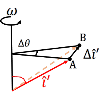
Figure 4.8 shows the rotation of the $\hat{\imath}^{\prime }$ coordinate axis.

Figure shows the rotation of the i-hat-prime axis. — Figure 4.8:The $\hat{\imath}^{\prime }$ coordinate is offset by an angle $\varphi$ from the rotation axis (angle in red). In time $\Delta t, \hat{\imath}^{\prime }$ moves from position $A$ to position $B$ due to rotation. The change in the vector position is shown by the angle $\Delta \hat{\imath}^{\prime }$ and angle $\Delta \theta$ .

From Figure 4.8, the $\hat{\imath}^{\prime }$ axis moves a distance $\Delta \hat{\imath}^{\prime }$ between points $A$ and $B$ in a time $\Delta t$ . That displacement in time $\Delta t$ is:

\Delta \hat{\imath}^{\prime }= (\hat{\imath}^{\prime }\sin \varphi)\Delta \theta

(40)

\frac{\Delta \hat{\imath}^{\prime}}{\Delta t} = (\hat{\imath}^{\prime}\sin \varphi) \frac{\Delta \theta}{\Delta t} =\Rightarrow \mathrm{divide} \mathrm{by} \Delta t

(41)

Assuming that $\Delta t$ is sufficiently short, we can set $\Delta t \rightarrow$ d $t, \Delta \hat{\imath}^{\prime }\rightarrow$ d $\hat{\imath}^{\prime }$ , and $\Delta \theta \rightarrow$ d $\theta$ :

\frac{\mathrm{d}\hat{\imath}^{\prime}}{\mathrm{d}t} = (\hat{\imath}^{\prime}\sin \varphi) \frac{\mathrm{d}\theta}{\mathrm{d}t}

(42)

\frac{\mathrm{d}\hat{\imath}^{\prime}}{\mathrm{d}t} = (\hat{\imath}^{\prime}\sin \varphi)\omega =\Rightarrow \omega = \frac{\mathrm{d}\theta}{\mathrm{d}t}

(43)

This form of this equation should look familiar. It looks like a vector cross product. Recall that $\vec{a} \times \vec{b} = ab\sin \theta$ , where $\theta$ is the angle between the vectors. So we can say that

\frac{\mathrm{d}\hat{\imath}^{\prime}}{\mathrm{d}t} = \vec{\omega} \times \hat{\imath}^{\prime}

(44)

You can apply similar arguments to get

\frac{\mathrm{d}\hat{\jmath}^{\prime}}{\mathrm{d}t} = \vec{\omega} \times \hat{\jmath}^{\prime}

(45)

\frac{\mathrm{d}\hat{k}^{\prime}}{\mathrm{d}t} = \vec{\omega} \times \hat{k}^{\prime}

(46)

Combining these definitions of the motion for the $S^{\prime }$ coordinates, we get:

\begin{aligned} x^{\prime} \frac{\mathrm{d}\hat{\imath}^{\prime}}{\mathrm{d}t} + y^{\prime} \frac{\mathrm{d}\hat{\jmath}^{\prime}}{\mathrm{d}t} + z^{\prime} \frac{\mathrm{d}\hat{k}^{\prime}}{\mathrm{d}t} &= x^{\prime}(\vec{\omega} \times \hat{\imath}^{\prime}) + y^{\prime}(\vec{\omega} \times \hat{\jmath}^{\prime}) + z^{\prime}(\vec{\omega} \times \hat{k}^{\prime}) \\ &= \vec{\omega} \times (x^{\prime }\hat{\imath}^{\prime }+ y^{\prime }\hat{\jmath}^{\prime }+ z^{\prime }\hat{k}^{\prime }) \end{aligned}

(47)

= \vec{\omega} \times \vec{r}^{\prime }

(48)

Thus, our coordinate transformation is:

\vec{v} = \vec{v}^{\prime }+ \vec{\omega} \times \vec{r}^{\prime }

(49)

where $\vec{v}$ is the velocity relative to the inertial frame, $\vec{v}^{\prime }$ is the velocity relative to the rotating frame, and $\vec{\omega} \times \vec{r}^{\prime }$ is the coordinate transformation of the rotating frame.

4.4.3 Coordinate System of a Rotating Frame: Acceleration¶

Before we solve for the acceleration, we are going to modify our velocity equation slightly so we don’t need to take the second time derivative of any of the position vectors. In Equation (4.3), we have $\vec{v} = \vec{v}^{\prime }+ \vec{\omega} \times \vec{r}^{\prime }$ . Since velocity is the time derivative of position, we can say,

\begin{aligned} \vec{v} &= \Bigg(\frac{\mathrm{d}\vec{r}}{\mathrm{d}t} \Bigg)_{I} \\ \vec{v}^{\prime}&= \Bigg(\frac{\mathrm{d}\vec{r}^{\prime}}{\mathrm{d}t} \Bigg)_{R} \end{aligned}

(50)

where the two differentials correspond to the time derivative of the position vector in the inertial frame (subscript “I”) and the time derivative of the position vector in the rotating frame (subscript “R”). That is, we do not take the time derivative of the unit vectors in either case because we are applying the time derivative in each of their frames (from the perspective of an observer in those frames, the unit vectors are fixed).

Coming back to our velocity Equation (4.3), we have:

\begin{aligned} \vec{v} &= \vec{v}^{\prime }+ \vec{\omega} \times \vec{r}^{\prime } \\ \Bigg(\frac{\mathrm{d}\vec{r}}{\mathrm{d}t} \Bigg)_{I}&= \Bigg(\frac{\mathrm{d}\vec{r}^{\prime}}{\mathrm{d}t} \Bigg)_{R}+ \vec{\omega} \times \vec{r}^{\prime} \end{aligned}

(51)

\Bigg(\frac{\mathrm{d}\vec{r}}{\mathrm{d}t} \Bigg)_{I}= \Bigg[\Bigg(\frac{\mathrm{d}}{\mathrm{d}t} \Bigg)_{R}+ \vec{\omega}\times \Bigg]\vec{r}^{\prime}

(52)

Recall however that $\vec{r} = \vec{r}^{\prime }$ since both frames have the same origin and same end point, $P$ . As a result, we can say that the above equation can be written as:

\left(\frac{\mathrm{d}\vec{r}}{\mathrm{d}t}\right)_{I} =\underbrace{\left[\left(\frac{\mathrm{d}}{\mathrm{d}t}\right)_{R} +\vec{\omega}\times\right]}_{\text{operator}}\vec{r}

(53)

where the term in front of $\vec{r}$ acts like a coordinate transformation operator on vector $\vec{r}$ to go from the rotating frame to the inertial frame. But you can technically apply an operator to any vector, it doesn’t have to be position. So if we apply this vector operator to $\vec{v}$ instead of $\vec{r}$ , we get acceleration in the inertial frame.

\Bigg(\frac{\mathrm{d}\vec{v}}{\mathrm{d}t} \Bigg)_{I}= \Bigg(\frac{\mathrm{d}\vec{v}}{\mathrm{d}t} \Bigg)_{R}+ \vec{\omega} \times \vec{v}

(54)

However, taking the time derivative of $\vec{v}$ in the rotating frame will require a coordinate transformation of the unit vectors. Fortunately, we can re-write $\vec{v}$ as $\vec{v}^{\prime }+ \vec{\omega} \times \vec{r}^{\prime }$ , which is relative to the rotating frame (so we don’t need to worry about the moving unit vectors).

\Bigg(\frac{\mathrm{d}\vec{v}}{\mathrm{d}t} \Bigg)_{I}= \Bigg(\frac{\mathrm{d}\vec{v}}{\mathrm{d}t} \Bigg)_{R}+ \vec{\omega} \times \vec{v}

(55)

\begin{aligned} &= \Bigg(\frac{\mathrm{d}}{\mathrm{d}t} \Bigg)_{R}(\vec{v}^{\prime}+ \vec{\omega} \times \vec{r}^{\prime}) + \vec{\omega} \times (\vec{v}^{\prime}+ \vec{\omega} \times \vec{r}^{\prime}) \\ &= \Bigg(\frac{\mathrm{d}\vec{v}^{\prime}}{\mathrm{d}t} \Bigg)_{R}+ \Bigg(\frac{\mathrm{d}\vec{\omega}}{\mathrm{d}t} \Bigg)_{R}\times \vec{r}^{\prime}+ \vec{\omega} \times \Bigg(\frac{\mathrm{d}\vec{r}^{\prime}}{\mathrm{d}t} \Bigg)_{R}+ \vec{\omega} \times \vec{v}^{\prime}+ \vec{\omega} \times (\vec{\omega} \times \vec{r}^{\prime}) \end{aligned}

(56)

This looks like a mess, but we can simplify it a bit. First, by definition, the accelerations in each reference frame are:

\begin{aligned} \vec{a} &= \Bigg(\frac{\mathrm{d}\vec{v}}{\mathrm{d}t} \Bigg)_{I} \\ \vec{a}^{\prime}&= \Bigg(\frac{\mathrm{d}\vec{v}^{\prime}}{\mathrm{d}t} \Bigg)_{R} \end{aligned}

(57)

where $\vec{a}$ is the acceleration of the point in the inertial frame and $\vec{a}^{\prime }$ is the acceleration of the point in the rotating frame.

In addition, recall that the velocity of the object from the perspective of the rotating frame:

\vec{v}^{\prime}= \Bigg(\frac{\mathrm{d}\vec{r}^{\prime}}{\mathrm{d}t} \Bigg)_{R}

(58)

Combining these definitions, our acceleration is:

\vec{a} = \vec{a}^{\prime}+ \Bigg(\frac{\mathrm{d}\vec{\omega}}{\mathrm{d}t} \Bigg)_{R}\times \vec{r}^{\prime}+ 2\vec{\omega} \times \vec{v}^{\prime}+ \vec{\omega} \times (\vec{\omega} \times \vec{r}^{\prime})

(59)

The only term that is still unclear is the time derivative of the angular velocity. If you apply the coordinate transformation operator from Equation 4.4 to $\vec{\omega}$ (recall that operators can be applied on any vector), you will get that

\Bigg(\frac{\mathrm{d}\vec{\omega}}{\mathrm{d}t} \Bigg)_{R}= \Bigg(\frac{\mathrm{d}\vec{\omega}}{\mathrm{d}t} \Bigg)_{I}

(60)

So we will define the time derivative of $\vec{\omega}$ as $\vec{\alpha}$ , which is the angular acceleration.

Thus, we obtain the equation for the coordinate transformation of:

\vec{a} = \vec{a}^{\prime }+ \vec{\alpha} \times \vec{r}^{\prime }+ 2\vec{\omega} \times \vec{v}^{\prime }+ \vec{\omega} \times (\vec{\omega} \times \vec{r}^{\prime })

(61)

Here $\vec{a} = \ddot{x}\hat{\imath} + \ddot{y}\hat{\jmath} + \ddot{z}\hat{k}$ and $\vec{a}^{\prime }= \ddot{x}^{\prime }\hat{\imath}^{\prime }+ \ddot{y}^{\prime }\hat{\jmath}^{\prime }+ \ddot{z}^{\prime }\hat{k}^{\prime }$ in Cartesian coordinates. That is, these are the accelerations as seen from the inertial frame and rotating frame, respectively. The remaining terms are additional forms of acceleration. These are the “fictitious forces” for a rotating non-inertial frame of reference.

4.5 Types of Acceleration and Fictitious Forces¶

Equation 4.5 equates the acceleration between an inertial frame and a non-inertial rotating frame where the two have the same origin. In practice, the origin of the rotating frame can move relative to the origin of the inertial frame. This motion would add a linear acceleration term that is independent of the rotation, so we can just add an additional acceleration term, $\vec{A}$ to represent the acceleration of the origin of the rotating frame as viewed by an observer in the inertial frame.

Thus, our final equation for the acceleration (relative to the non-inertial frame) is:

\underbrace{\vec{a}'}_{1} =\underbrace{\vec{a}}_{2} -\underbrace{\vec{\alpha}\times\vec{r}}_{3} -\underbrace{2\vec{\omega}\times\vec{v}'}_{4} -\underbrace{\vec{\omega}\times(\vec{\omega}\times\vec{r})}_{5} -\underbrace{\vec{A}}_{6}

(63)

Linear acceleration in the rotating frame (what an observer in the rotating frame would measure as the acceleration). This would be equivalent to the net acceleration from the perspective of the rotating frame.
Linear acceleration in the inertial frame (what an observer in the inertial frame would measure as the acceleration). This would be equivalent to the net acceleration from the perspective of the inertial frame.

Azimuthal acceleration. This is a fictitious force acceleration that arises due to a change in the angular velocity of rotation (either magnitude or direction). Some call this the transverse acceleration.
Coriolis acceleration. This is a fictitious force acceleration if you have an object moving in a rotating frame.
Centrifugal acceleration. This is a fictitious force acceleration if you have an object offset from the origin of a rotating frame.
Translational acceleration. This is a fictitious force acceleration that represents how the origin of the rotating frame moves relative to the origin of the inertial frame.

To solve for the force in the rotating frame, multiply all the accelerations by the mass, $m$ :

m\vec{a}^{\prime }= m\vec{a} - m\vec{\alpha} \times \vec{r} - 2m\vec{\omega} \times \vec{v}^{\prime }- m\vec{\omega} \times (\vec{\omega} \times \vec{r}) - m\vec{A}

(64)

m\vec{a}^{\prime }= \sum \vec{F}_{I}+ \vec{F}_{az}+ \vec{F}_{Cor}+ \vec{F}_{cent}+ \vec{F}_{trans}

(65)

where $\sum \vec{F}_{I}$ is the net force in the inertial frame and the remaining terms are all the fictitious forces. Note that for a given problem, not all fictitious forces may be present. You will need to consider the physics in the problem to identify which ones are applicable.

4.6 Simple Example of a Rotating Reference Frame¶

This chapter looks at simple cases of rotating reference frames. We will get to more complicated cases in Chapter 5.

star. There is a single force, gravity, acting on the particle.

\sum \vec{F}_{I}= - \frac{GMm}{R^{2}} \hat{r} = m\vec{a}

(66)

The equation of motion for circular rotation is $r$ = constant, so that $\dot{r} = \ddot{r}$ = 0. The motion comes entirely from a change in angle. For circular motion, we can use the centripetal acceleration, $\vec{a} = -\omega ^{2}R\hat{r}$ to describe the circular motion. Recall that this equation comes directly from plane-polar coordinates (see Chapter 1.2).

- \frac{GMm}{R^{2}} \hat{r} = -m\omega ^{2}R\hat{r}

(67)

Rotating Frame: In the rotating frame, an observer sitting on the particle doesn’t think the particle is moving. So this observer would measure no rotation and no acceleration relative to their position. So this observer would measure:

m\vec{a}^{\prime }= 0

(68)

But this observer has not considered that they are on a rotating reference frame. As a result, they need to consider the fictitious forces that come with that frame.Fortunately, many of the terms are equal to zero.

m\vec{a}'=\sum\vec{F}_{I} -m\vec{\alpha}\times\vec{r} -2m\vec{\omega}\times\vec{v}' -m\vec{\omega}\times(\vec{\omega}\times\vec{r}) -m\vec{A},

(69)

There is no angular acceleration $(\alpha$ = 0), the person is not moving within the rotating frame $(\vec{v}^{\prime }$ = 0), and the origins are not changing $(\vec{A}$ = 0). The only fictitious force left is the centrifugal force. Therefore,

0=\sum\vec{F}_{I} -\underbrace{m\vec{\omega}\times(\vec{\omega}\times\vec{r})}_{\vec{F}_{cent}}

(70)

For this circular rotation, the angular velocity and radial vectors are perpendicular to each other. Thus, $F_{cent}$ has a magnitude of $m\omega ^{2}R$ . You’ll notice that this force has the same magnitude as the centripetal acceleration in the inertial frame.

What about the direction of the centrifugal force? In the rotating frame, the centrifugal force points outward from the origin. This makes sense, since fictitious forces act in the opposite direction to the acceleration relative to the inertial frame (equivalence principle). The centripetal acceleration always points inward. The figure below shows a breakdown of the $\vec{\omega} \times (\vec{\omega} \times \vec{r})$ cross product terms.

4.7 Summary¶

Key Takeaways

This chapter introduces the concepts of inertial and non-inertial frames. Inertial frames are reference frames that are either stationary or move with a constant velocity, whereas non-inertial frames are either accelerating or rotating.

To solve physics problems in non-inertial and rotating frames, we introduced the concept of fictitious forces. These are not real forces, in the sense that they arise from any specific interactions. They are forces that appear to act on an object to explain its properties. The fictitious force always acts opposite the direction of the acceleration (equivalence principle).

\vec{F}_{fic}= -m\vec{a}_{S^{\prime }S}

(73)

In this chapter, we derive the coordinate transformations between inertial and noninertial frames. The general case is,

\vec{a}^{\prime }= \vec{a} - \vec{\alpha} \times \vec{r}^{\prime }- 2\vec{\omega} \times \vec{v}^{\prime }- \vec{\omega} \times (\vec{\omega} \times \vec{r}^{\prime }) - \vec{A}

(74)

If there is no rotation, then the coordinate transformation is:

\vec{a}^{\prime }= \vec{a} - \vec{A}

(75)

Due to the extra acceleration terms, Newton’s second law in a non-inertial frame needs to include extra “force” terms from the fictitious forces:

\sum \vec{F}_{S^{\prime }}= \sum \vec{F}_{S}+ F_{fic}

(76)

Using the naming convention for the different fictitious forces, Newton’s second law in a non-inertial frame is:

m\vec{a}^{\prime }= \sum \vec{F}_{I}+ \vec{F}_{az}+ \vec{F}_{Cor}+ \vec{F}_{cent}+ \vec{F}_{trans}

(77)

Depending on your physics problem, it can be easier to solve a question in the noninertial frame than in the inertial frame. Recognizing which frame to use is part of the challenge. When working on the practice problems, think about which frame of reference is easier to work with.

Important Equations

Fictitious Forces:

\sum \vec{F}_{S^{\prime }}= \sum \vec{F}_{S}+ F_{fic}

(78)

\vec{F}_{fic}= -m\vec{a}_{S^{\prime }S}

(79)

Coordinate Transformation for velocity:

\vec{v} = \vec{v}^{\prime }+ \vec{\omega} \times \vec{r}^{\prime }

(80)

Acceleration in a Rotating Frame:

\vec{a}^{\prime }= \vec{a} - \vec{\alpha} \times \vec{r}^{\prime }- 2\vec{\omega} \times \vec{v}^{\prime }- \vec{\omega} \times (\vec{\omega} \times \vec{r}^{\prime }) - \vec{A}

(81)

Newton’s Second Law in a Rotating Frame:

m\vec{a}^{\prime }= \sum \vec{F}_{I}+ \vec{F}_{az}+ \vec{F}_{Cor}+ \vec{F}_{cent}+ \vec{F}_{trans}

(82)

4.8 Practice Problems¶

See Appendix C for answers to the practice problems.

Practice Problem 4-9

Consider two astronauts in space far from any source of gravity. The spaceship is accelerating upwards (relative to an inertial observer watching the spaceship) at an acceleration of $a = 9.8$ m $\mathrm{s}^{-2}$ . Inside, the two astronauts are throwing a ball back and forth. The ball has a mass $m$ and the two astronauts are 10 m away from each other.

Figure 4.12:Figure for Problem 4-9.

a) In the frame of the two astronauts (the non-inertial frame), what is the magnitude and direction of the fictitious force acting on the ball?

b) In the frame of the two astronauts (the non-inertial frame), what is the effective gravity acting on the ball? Draw a free-body diagram.

c) Astronaut 1 is throwing the ball to Astronaut 2. In the frame of the two astronauts (the non-inertial frame), what is the minimum speed needed for the ball to travel the 10 m between the two astronauts and how long does it take to reach Astronaut 2? You can assume that Astronaut 1 has a height of 2 m and tosses the ball to Astronaut 2 at an angle of 0 deg relative to the horizontal.

d) Now consider an observer that is outside of the spaceship and not moving (the inertial frame). What forces are acting on the ball after Astronaut 1 throws it?

e) Solve for the minimum speed and time from the perspective of an observer in the inertial frame. Do you get the same answers as c)?

f) Describe the trajectory of the ball in the frame of the inertial observer and the frame of the two astronauts?