1. Calculus and Vectors

This chapter reviews basic calculus and vector notation and coordinate systems. Please also refer to Appendix A for helpful equations and identities.

1.1 Coordinates and Motion in Vector Notation¶

1.1.1 Linear Motion¶

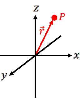
For linear motion, we can use the Cartesian coordinate system. The position of an object is described by a vector $\vec{r}$ in $x, y$, and $z$, the linear velocity of the object is the time derivative of position, and the linear acceleration is the time derivative of velocity.

The equations of linear motion in 1-D:

Equations of linear motion in 3-D:

The above equations highlight that there are several ways to write a parameter in vector notation. For example, $\vec{r}$ can be expressed as $x\hat{\imath} + y\hat{\jmath} + z\hat{k}$ or $\langle x,y,z\rangle$. You should try to be consistent within a problem so that there is less chance for confusion or error in your solutions.

1.1.2 Rotational Motion¶

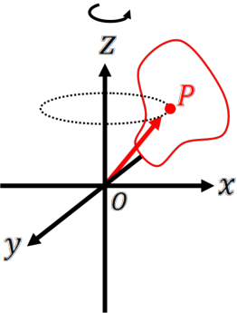
Rotational motion is when you have a body spinning about a rotation axis.

For rotational motion, it is useful to describe the motion in terms of angles: angular position $(\theta)$, angular velocity $(\omega)$, and angular acceleration $(\alpha)$. Note that a radius $r$ is also necessary to describe the motion, and we will assume this is constant for now. For this coordinate system to work, you need a reference axis (reference point).

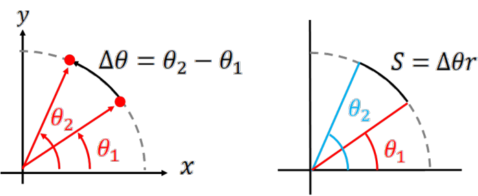
Consider the figure below. In time $t_{1}$ to $t_{2}$ the object has rotated from the first position at $\theta _{1}$ to the second position at $\theta _{2}$. The distance from the origin to both points (radius) is constant. Thus, the angular position that the object moves is $\Delta \theta = \theta _{2}- \theta _{1}$ in time $\Delta t = t_{2}- t_{1}$. The distance traveled is the arc, $s$, as traced out by the angle $\Delta \theta$.

For angular motion, we generally measure angles in radians not degrees. One complete circle is when $\theta = 2\pi$ or $s = 2\pi r$ (the perimeter of a circle). Note that a complete rotation does not start back at $\theta$ = 0.

$2\pi$ rad = $360^{\circ}$ = 1 revolution

1 rad = $57.296^{\circ}= 0.159$ revolutions

The average angular velocity of the object is then given by $\bar{\omega} = \frac{\Delta \theta}{\Delta t}$. As we shrink $\Delta t$ to a very small time interval $(\Delta t \rightarrow$ d$t)$, then we get the instantaneous angular velocity or the angular velocity, $\omega$. The angular velocity is given by the time derivative of $\theta$ and the angular acceleration is given by the time derivative of the angular velocity.

The units of $\omega$ are rad $\mathrm{s}^{-1}$ and the units of $\alpha$ are rad $\mathrm{s}^{-2}$, although we often drop the radians and give $\mathrm{s}^{-1}$ and $\mathrm{s}^{-2}$, respectively. If you see $\mathrm{s}^{-1}$ or $\mathrm{s}^{-2}$ for $\omega$ and $\alpha$, the radians are implied.

For a rigid body, all points in the object move with the same angular velocity and angular acceleration because every point is moving together (the object doesn’t deform during rotation).

1.2 Introduction to Plane Polar Coordinates¶

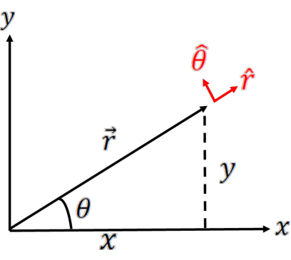
In cases of circular motion, it is often easier to solve a problem by changing your coordinate system from Cartesian plane $(x,y)$ to polar coordinates $(r,\theta)$. The two coordinate systems are connected, where $x = r\cos \theta$ and $y = r\sin \theta$, where $r$ is the radius length and $\theta$ is the polar angle (see Figure 1.4). Solving for $r$ and $\theta$, we get:

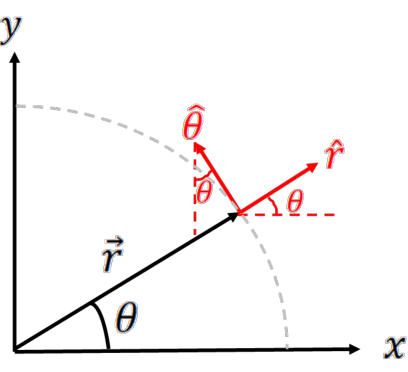
Of course, $r$ and $\theta$ are the polar coordinates (scalars), with unit vectors $\hat{r}$ and $\hat{\theta}$, where $\hat{r}$ points away from the origin of the system and $\hat{\theta}$ is orthogonal to $\hat{r}$ in the counter-clockwise direction (usually). Note that the hat symbol indicates a unit vector (direction only). Figure 1.4 shows these vector directions.

The position vector in plane polar coordinates can be written as $\vec{r} = r\hat{r}$ and the angle vector can be written as $\vec{\theta} = \theta \hat{\theta}$ .

Now we want to find an equation for $\vec{v}$ and $\vec{a}$ in polar coordinates instead of Cartesian coordinates. This is a variation of how we defined velocity and acceleration previously (because previously we used Cartesian coordinates).

Let’s look at velocity first.

where $\frac{\mathrm{d}\hat{r}}{\mathrm{d}t} \not =$ 0. Consider the line moving in Figure 1.4. The $\hat{r}$ unit vector will point in a different direction as the radius vector moves around the circle.

Figure 1.5 defines the $\hat{r}$ and $\hat{\theta}$ unit vectors in terms of Cartesian axes. Both $\hat{r}$ and $\hat{\theta}$ have components in $x$ and $y$.

Note that the Cartesian unit vectors $(\hat{\imath}, \hat{\jmath}$ ) are fixed, whereas the polar-axes $(\hat{r}, \hat{\theta}$ ) are moving relative to them because the radial vector is moving.

If we take the derivative of $\hat{r}$ with respect to time, we get:

The above equation applies a full time derivative to $\hat{r}$ , which means that you must not only take the time derivative of $\cos \theta$ and $\sin \theta$, but also time derivative of $\theta$. See the textbook repository for a video showing the difference between full and partial derivatives.

Now that we have $\frac{\mathrm{d}\hat{r}}{\mathrm{d}t}$, we can go back to our velocity equation from before. For polar coordinates we get:

where the first term is the radial velocity component $\vec{v}_{r}$ and the second term is the tangential velocity component $\vec{v}_{\theta}$. The radial velocity component indicates how the point is moving in and out along the direction of the radius vector, whereas the tangential velocity component of the motion describes how the point is moving along a circle (motion that is tangent to the radius vector). For circular motion, the radius is constant, such that $\frac{\mathrm{d}r}{\mathrm{d}t}=0$ and you get $\vec{v}_{circ}= r\omega \hat{\theta}$ .

By definition the speed (or $|\vec{v}|$) is given by $\sqrt{\vec{v}\cdot\vec{v}}=\sqrt{v_{r}^{2}+v_{\theta}^{2}}=\sqrt{v_{r}^{2}+(r\omega)^{2}}$, using the vector dot product (see also, Chapter 1.5.1).

We can also take the time derivative of $\hat{\theta}$ , using the definition of $\hat{\theta}$ in Cartesian coordinates.

For acceleration, we want the time derivative of velocity. Following a similar procedure,

where the first term is the acceleration in the radial direction $(a_{r})$ and the second term is the acceleration in the tangential direction $(a_{\theta})$. That is:

These acceleration terms are key in rotating reference frames (Chapter 5).

1.3 Equations of Motion¶

In the previous section, we defined the positions, velocities, and accelerations for linear and circular motion. To describe the motion, however, you need to solve these equations.

The solutions to these integrals depends on how the system moves with time. For example, consider the case when $\alpha$ and $\vec{a}$ are constant with time. Let’s look at the case of linear motion with constant acceleration in 1-D so that we can drop the vector notation.

where $a_x$ is constant by definition and $C_{1}$ is a constant of integration.

where we have substituted the equation for $v_x$. Integrating gives

where $C_{2}$ is a constant of integration.

The constant $C_{1}$ is the initial velocity $v_{x,0}$ (at $t$ = 0) and $C_{2}$ is the initial position $x_{0}$ (at $t$ = 0). Subbing in those definitions for the constants of integration, we get:

Hopefully these equations look familiar. Of course, since position and velocity are vector quantities, you need to solve for the motion along the different coordinate axes (e.g., $x,y,z)$ separately. For example, the acceleration may be zero along one axis and non-zero along another axis (e.g., such is the case with gravity).

Note that if you take the time derivative of $x = \frac{1}{2} a_{x}t^{2}+v_{x,0}t+x_{0}$, you recover the equation for $v_{x}= a_{x}t + v_{x,0}$ as you should. In general, it is a good idea to check the consistency of your equations.

1.4 Linear and Rotational Motion¶

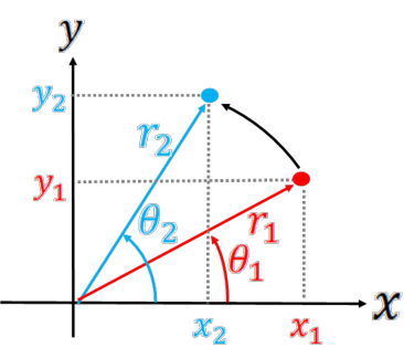
We can also connect circular motion to linear motion. Consider two points associated with rotational motion with a circular radius of $r_{0}$ as shown below.

We can write the radius vectors in terms of their $x$ and $y$ values. For example, $x_{1}= r_{1}\cos \theta _{1}$ and $y_{1}= r_{1}\sin \theta _{1}$. The same can be applied to the second position. In vector form, we get:

For circular motion, $\theta$ changes with time. Let’s consider the simplest case where $\dot{\theta} = \omega$ = constant, such that we can solve for $\theta (t)$ as $\theta = \int \omega$d$t = \omega t + \theta _{0}$, where $\theta _{0}$ is a constant of integration and represents the initial angle. It is often convenient to define the initial angle as $\theta _{0}$ = 0 so $\theta (t) = \omega t$. Therefore, we get:

We can then look at the velocity and acceleration of the system by just taking the time derivatives of $\vec{r}$.

Note that we are using the $y$ axis only at this time because all the motion is in the vertical.

1. What is the maximum height that the ball reaches? This is the height at point B in Figure 1.7. This problem is a linear motion question with constant acceleration. We just solved that equation in Section 1.3, so we will need to use the equation, $y = \frac{1}{2} at^{2}+ v_{y,0}t + r_{0}$ to solve for $y$ when the ball is at its highest point. We aren’t given that time when this happens, but we can solve for it, because when the ball has reached its maximum height, $v_{y}$ = 0 (requirement of the physics). So the first step is to get the time when the ball has reached its maximum height.

For simplicity, we can drop the vector notation because everything is happening in 1-D. Here positive corresponds to $+\hat{y}$ and negative corresponds to $-\hat{y}$ .

So now we have the time when the ball reaches the maximum height. We can put this time into our distance equation to solve for the maximum height.

Now we have our equation for the maximum height given our initial velocity $v_{y,0}$ and initial height $r_{0}$. This is the generic solution for all initial values of $v_{y,0}$ and $r_{0}$. If you are given these quantities, you can plug them in to solve the problem.

2. How long does it take for the ball to reach the ground? So this is at the end of the motion (point D in Figure 1.7). We don’t know the speed at which the ball reaches the ground or the time, but we do know the ball hits the ground when $y$ = 0. So we want to solve for the time when $y$ = 0. Using the height equation, we get $y = - \frac{1}{2} gt^{2}+ v_{y,0}t + r_{0}$ = 0, which is a quadratic equation. The solution for a quadratic equation of the form 0 = $Ax^{2}+ Bx + C$ is:

In this case, $t$ is our variable, $A = - \frac{1}{2} g, B = v_{y,0}$, and $C = r_{0}$. Plugging those numbers in gives:

There are two solutions. Since $2gr_{0}$ is positive, the term $\sqrt{v_{y,0}^{2}+2gr_{0}}>v_{y,0}$ for all values of $v_{y,0}$ and $r_{0}$. So there will be one value of $t > 0$ and one value of $t < 0$. The latter case $(t < 0)$ is unphysical given the set up of this problem, however. While it mathematically solves the problem, we know that the ball’s motion started from a height $r_{0}$ at $t$ = 0. Effectively, the $t < 0$ case corresponds to the time when the ball would need to be thrown from $y$ = 0 such that it has a speed of $v_{y,0}$ at $t$ = 0 and height $r_{0}$. But that wasn’t our question, so we are instead interested in the $t > 0$ case.

So our solution to this problem is:

Here we drop the $-$ case because it is unphysical.

1.5 Vector Calculus¶

1.5.1 Vector Dot Product¶

For any two vectors, $\vec{a} = x_{a}\hat{\imath} + y_{a}\hat{\jmath} + z_{a}\hat{k}$ and $\vec{b} = x_{b}\hat{\imath} + y_{b}\hat{\jmath} + z_{b}\hat{k}$ , the vector dot product (also called the vector scalar product) is given by:

Since the dot product is just scalar multiplication of terms, vector order does not matter

In principle, the dot product represents the projection of one vector onto the other. For example, when you want to calculate the $x-$component of a vector, you take the projection of that vector on the $x-$axis. This is equivalent to $\vec{a} \cdot \hat{\imath}$, where only the $x-$component is retained.

The dot product can also be expressed as:

where $|\vec{a}|$ is the magnitude of $\vec{a}, |\vec{b}|$ is the magnitude of $\vec{b}$ and $\theta$ is the angle between the two vectors when the vectors are tail-to-tail. So the angle between any two vectors can be calculated from:

A vector magnitude is given by:

which is essentially the dot product of a vector with itself $(\theta$ = 0).

1.5.2 Vector Cross Product¶

For any two vectors, $\vec{a}$ and $\vec{b}$, the vector cross product is given by:

Unlike the dot product, the vector cross product results in a vector, which has both magnitude and direction, and the vector $\vec{c}$ is perpendicular to both $\vec{a}$ and $\vec{b}$. In other words, the vector cross product $\vec{c}$ is normal (perpendicular) to a plane that is defined by $\vec{a}$ and $\vec{b}$.

The magnitude of $\vec{c}$ can be given as:

where $\theta$ is the angle between the two vectors when the vectors are tail-to-tail. But this is only the magnitude. To get the direction of the cross product, you can use one of two methods: (1) the right hand rule (RHR) or (2) the matrix determinant method to solve the vector cross product.

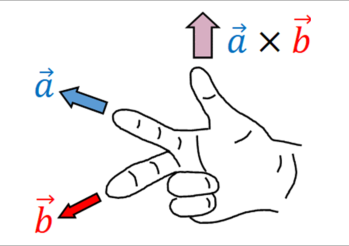
Figure 1.8 shows how to solve for the cross product direction with the RHR.

The matrix determinant method gives you the full vector solution for the cross product:

For the vector cross product, order matters. Here are a few helpful identities:

1.6 Approximations¶

In physics, you can often make approximations to simplify the math based on the conditions of your system. For example, if you have a complicated force acting on a system, but you are only interested in short distances or short times, you can often simplify the equation for that force making the calculations easier. Deviations between the true value (considering the full complicated force equation) and the approximation (with the simplified force equation) would be considered small, such that you get a good idea of how the system will move without needing to do the complicated math. (Of course, with some high-precision physics, you cannot make this approximation.)

A very common approach is to use the Taylor series expansion. The idea here is that any function can be broken up into a series of polynomials following:

where $f(x)$ is the function and $x_{0}$ is a reference value for the function and the ! symbol is the factorial symbol. That is $f(x)$ describes the entire function for all values $x$, whereas $f(x_{0})$ is the value of the function at the specific value of $x = x_{0}$. See Appendix B.2 for more details and other approximation techniques.

For Equation 1.5, consider values of $x \approx x_{0}$. That is, you are only looking at cases of your variable, $x$ when it is close to your reference value. In this case, $x-x_{0}$ is small. Thus, higher order terms like $(x-x_{0})^{2}$ and $(x-x_{0})^{3}$ are very small and can be dropped. Suddenly, your function has become very simple.

Let’s look at an example. Consider the Taylor series expansion for $e^{x}$ for small values of $x$. In this case, we can set $x_{0}$ = 0 because we are looking at small values of $x$. The expansion is:

where $f^{\prime }(0)$ means take the derivative of $f(x)$ with respect to $x$ and evaluate that for $x$ = 0. For $f = e^{x}$, we have:

and so forth. Taking these terms, we can approximate the solution to $e^{x}$ at $x \approx 0$ as:

where we drop the higher order terms because if $x$ is small $(|x| \ll$ 1), then the higher order terms which have $x^{2}$ and $x^{3}$ become negligible. A function of 1 + $x$ is much simpler to work with than a function of $e^{x}$. This highlights the power of a Taylor series expansion.

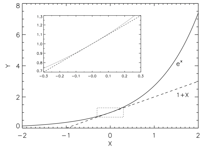
Figure 1.9 demonstrates this approximation. The figure compares a function of $e^{x}$ with a function of $1+x$. For small values of $x$ (such as $-0.3 < x < 0.3)$, the two functions are very similar. For larger values of $x$, however, the approximation breaks down. Note, however that you can include additional higher order terms when necessary. That is, $e^{x}\approx 1+x+ \frac{1}{2} x^{2}$ would give a better approximation than $e^{x}\approx 1 + x$.

See Appendix A.3 for a list of common Taylor series approximations and Appendix B.2 for more details on this method and other approximations. Taylor series approximations may seem confusing at first, but they can work for you when applied properly. When we use the Taylor approximation throughout this text, think about why we are using it and how the approximation simplifies the calculations.

1.7 Real-World Application: LIGO¶

One of the simplest, fundamental concepts in physics is the case of constant motion where $d = vt$. And this basic equation is at the core of one of the most ground-breaking discoveries in the 21st century, gravitational waves.

First predicted by Einstein in 1916, gravitational waves are a natural outcome of General Relativity and can be described as “ripples” in spacetime. They are incredibly small in

magnitude, where strong gravitational waves have magnitudes on the order of 10^-18 m, which is around one thousandth the diameter of a proton. With the level of sensitivity needed, it was roughly a century between prediction and detection.

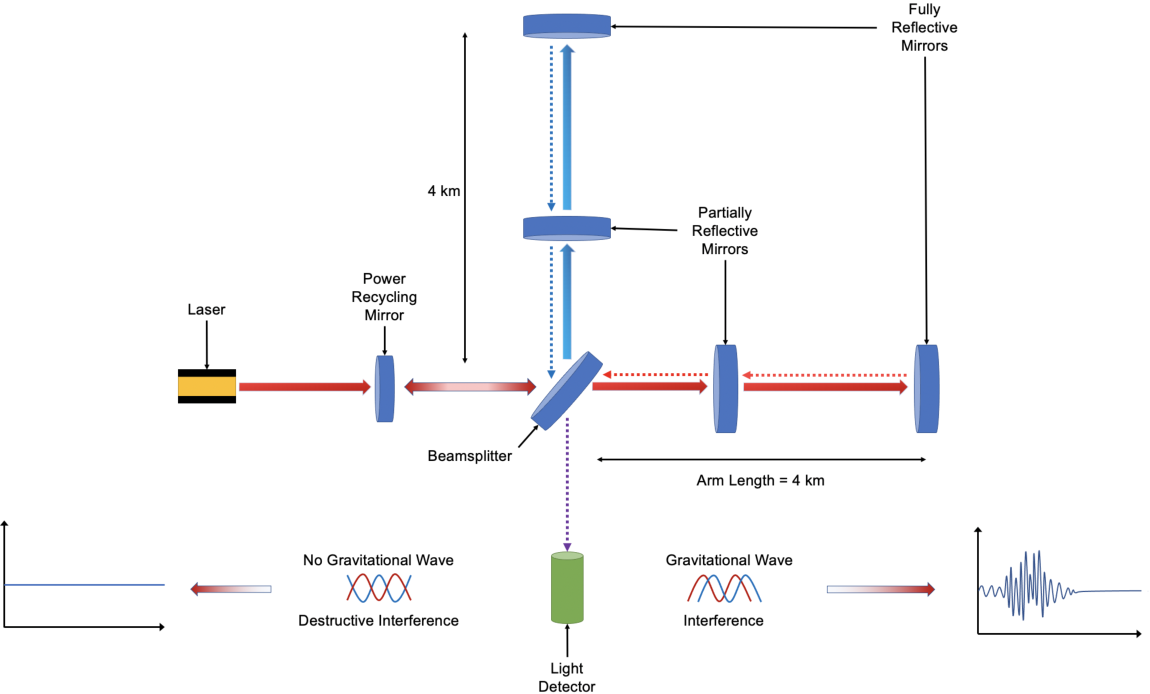
The first gravitational waves were detected on September 14, 2015 by the Laser Interferometer Gravitational-wave Observatory (LIGO) experiment. The experiment itself uses interferometry where identical laser beams reflect off mirrors and then converge on a detector producing an interference pattern (see Figure 1.10). When a gravitational wave passes through the Earth, it temporarily warps space and changes the distance between the mirrors which subsequently changes the arrival time of the reflected beams at the detector. LIGO can detect a change in distance between its mirrors on the order of 10^-19 m.

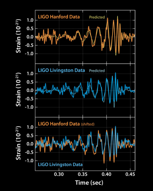
The slight change in distance from a passing gravitational wave alters the interference pattern measured at the detector. Figure 1.11 shows the gravitational wave signal from the first detection, which was generated by a pair of merging intermediate-mass black holes located 1.3 billion light years away. The interference pattern is often described as a “chirp”, because it rises to higher frequencies toward the end. Research into gravitational waves includes LIGO in the USA, VIRGO in Italy, and GEO600 in Germany, with a third site, KAGRA, under construction in Japan. Multiple experiments all over the world are necessary to pinpoint the direction of the gravitational wave events because each site will

measure a difference in signal and arrival time.

LIGO is an international collaboration including more than 1200 scientists from over 100 institutions located in 18 different countries. The ground-breaking discovery has significant implications for general relativity, black holes, and our universe. But recall that the basic principle at the heart of this experiment is a change in arrival time from a change in distance.

For more information: The LIGO Scientific Collaboration website has a lot of information about the original detection and process. This video translated the merging event into a sound bite that showcases the “chirp” from the merger. Sky & Telescope also has a nice article (with lots of links) describing the first detection.

1.8 Summary¶

1.9 Practice Problems¶

See Appendix C for answers to the practice problems.