Ch 1 Python Exercises: Approximations¶

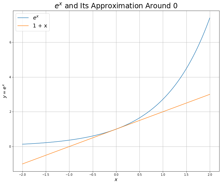
Below, you’ll find the basic code used for Figure 1.9 in the text. Using this code and either the basic approximations found in Appendix A or the Taylor Series approximation formula found in Appendix C, try the following approximations (consider x as close to 0 unless otherwise specified):

f(x) = $e^{-x^2}$
f(x) = $2e^{x^2}$
f(x) = $2e^{2x^3}$
f(x) = $\tan{x}$
f(x) = $\ln{(1 + x)}$
f(x) = $e^x$ for x close to 2

Try with both 2- and 3-term Taylor approximations. Note that there is also code for a more complicated example available in the text’s Python library.

import matplotlib.pyplot as plt              # for ease of use
import numpy as np                           # for the exponential function

plt.rcParams['figure.figsize'] = 12.5,10     # default plot size

# The basic plot for Figure 1.9

# define x for a nice, smooth curve
# Note that the -2 and 2 can be adjusted depending on how closely you want
# to look at the approximation.
x = np.linspace(-2, 2, 1000)

plt.figure()                               # set up the plot
plt.plot(x, np.exp(x), label = "$e^x$")    # the actual plot for e^x
plt.plot(x, (1 + x), label = "1 + x")      # two-term approximation

# three-term approximation if you'd like to see it
# plt.plot(x, (1 + x + 0.5*x**2), label = "1 + x + 0.5$x^2$")

# give the plot a title
plt.title("$e^x$ and Its Approximation Around 0", fontsize = 24)

plt.xlabel("$x$", fontsize = 16)           # label the axes
plt.ylabel("$y = e^x$", fontsize = 16)
plt.legend(fontsize = 18)                  # add a legend
plt.grid()                                 # grid lines

plt.show()                                 # display the result