Ch 2 Python Exercises¶

Example Code.

Exercises:

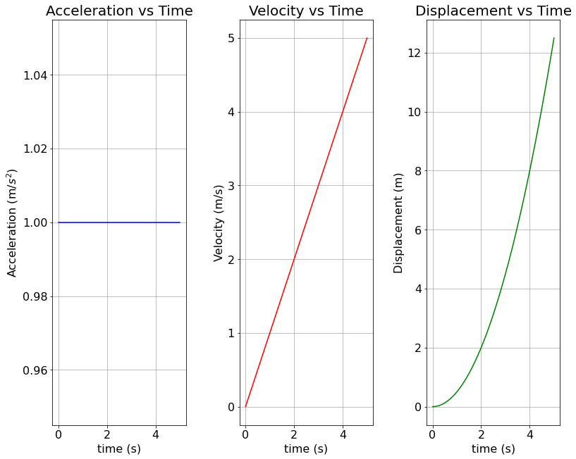
Constant Acceleration (shown in full)
1. For $v_0$ = 10 m/s and a = 9.8 m/s $^2$ , plot displacement, velocity, and acceleration for the first 3 seconds. Assume initial displacement is zero.
2. For $v_0$ = 10 m/s and $\theta$ = $45^{\circ}$ , plot displacement, velocity, and acceleration for horizontal and vertical components for the first five seconds.
Variable Acceleration (for practice)
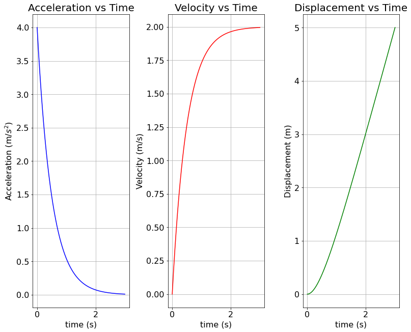
1. Adapt the example code for Variable Acceleration ( $a = 4e^{-2t}$ ) to plot acceleration, velocity, and displacement for starting conditions of v = 5.0 m/s, x = 3 m
2. Consider an alien parachutist of mass m jumping out of a hoverplane on their remarkably Earth-like home planet. If their initial vertical velocity is 0 m/s, taking g = 10 m/s and the variable acceleration due to air resistance as $F_{drag} = -0.2mv$ ,
  1. Find the Terminal Velocity, i.e. the velocity when their acceleration reaches zero.
  2. Have Python plot their velocity and acceleration for the first minute of their fall.

Note: all units used are SI standard units.

import matplotlib.pyplot as plt              # for ease of use
import numpy as np                           # for the needed math functions

plt.rcParams['figure.figsize'] = 12.5,10     # default plot size

Important Constant Acceleration Equations¶

$v = v_0 + at$
$x = x_0 + v_0t + 0.5at^2$
$v^2 = v_0^2 + 2a(x-x_0)$

2-D Velocity Components¶

$v_x = v_0\cos{\theta}$
$v_y = v_0\sin{\theta}$

Where $\theta$ is the angle above the horizontal.

Useful Python functions:

np.sin(x)
np.cos(x)
np.pi Where x is the input value in radians.

# The Example code for Constant Acceleration

# set initial conditions
x0, v0 = 0, 0

# define the Velocity function
def Velocity(t):
    return v0 + a * t

# define the Displacement function
def Displacement(t):
    return x0 + v0 * t + 0.5 * a * t**2

t = np.linspace(0, 5, 1000)                     # define t for smooth curve
a = np.full(1000,1)                             # acceleration is constant

# Display as three separate plots

plt.figure()                                    # set up the plot

plt.rcParams.update({'font.size': 16})

plt.subplot(1, 3, 1) # Acceleration in first column
plt.plot(t, a, color = "b")
plt.title("Acceleration vs Time", fontsize = 20)
plt.xlabel("time (s)", fontsize = 16)
plt.ylabel("Acceleration (m/$s^2$)", fontsize = 16)
plt.grid()

plt.subplot(1, 3, 2) # Velocity in second column
plt.plot(t, Velocity(t), color = "r")
plt.title("Velocity vs Time", fontsize = 20)
plt.xlabel("time (s)", fontsize = 16)
plt.ylabel("Velocity (m/s)", fontsize = 16)
plt.grid()

plt.subplot(1, 3, 3) # Displacement in third column
plt.plot(t, Displacement(t), color = "g")
plt.title("Displacement vs Time", fontsize = 20)
plt.xlabel("time (s)", fontsize = 16)
plt.ylabel("Displacement (m)", fontsize = 16)
plt.grid()

plt.subplots_adjust(left=0.1, bottom=0.1, right=0.9,
                    top=0.9, wspace=0.4, hspace=0.4)

plt.show()

# The Example code for Variable Acceleration
# Integration solved for initial conditions: x0 = 0, v0 = 0

# define the Acceleration function
def VAccel(t):
    return 4 * np.exp(-2*t)

# define the Velocity function
def VVel(t):
    return 2 - 2 * np.exp(-2*t)

# define the Displacement function
def VDisp(t):
    return np.exp(-2*t) + 2 * t - 1

t = np.linspace(0, 3, 1000)                      # define t for smooth curve

plt.rcParams.update({'font.size': 16})

plt.subplot(1, 3, 1) # Acceleration in first column
plt.plot(t, VAccel(t), color = "b")
plt.title("Acceleration vs Time", fontsize = 20)
plt.xlabel("time (s)", fontsize = 16)
plt.ylabel("Acceleration (m/$s^2$)", fontsize = 16)
plt.grid()

plt.subplot(1, 3, 2) # Velocity in second column
plt.plot(t, VVel(t), color = "r")
plt.title("Velocity vs Time", fontsize = 20)
plt.xlabel("time (s)", fontsize = 16)
plt.ylabel("Velocity (m/s)", fontsize = 16)
plt.grid()

plt.subplot(1, 3, 3) # Displacement in third column
plt.plot(t, VDisp(t), color = "g")
plt.title("Displacement vs Time", fontsize = 20)
plt.xlabel("time (s)", fontsize = 16)
plt.ylabel("Displacement (m)", fontsize = 16)
plt.grid()

plt.subplots_adjust(left=0.1, bottom=0.1, right=0.9,
                    top=0.9, wspace=0.4, hspace=0.4)

plt.show()