8. Work and Energy

In this chapter, we will switch to using energy to solve physical problems instead of Newton’s laws and momentum. We will review the concepts of work, kinetic energy, and potential energy, and we will introduce conservative forces.

8.1 Introduction to Work and Energy¶

When a force is applied to an object such that it moves a displacement of $\Delta \vec{r}$, work is done by that force. Work is defined as:

where $\vec{F}$ is the force and $\mathrm{d}\vec{r}$ represents a small displacement.

If the force is constant, then you can simplify the above equations to:

where $\Delta \vec{r}$ represents the displacement between two points, $r_{1}$ and $r_{2}$. Alternatively, the vector dot product can be solved following $\vec{F} \cdot \Delta \vec{r} = F\Delta r\cos \theta$, where $\theta$ is the angle between the two vectors.

If $\vec{F}$ and $\mathrm{d}\vec{r}$ are parallel $(\theta$ = 0), then the force is acting in the same direction as the displacement and the force does maximum positive work. If the force is perpendicular to the displacement $(\theta = \frac{\pi}{2})$, then the force does zero work. That is, the force is not responsible for the displacement and contributed no work to that displacement. If the force

is antiparallel to the displacement $(\theta = \pi)$, then the force does maximum negative work (the force acts to counter the motion as much as it can).

Work is a scalar quantity. It has magnitude but no direction. Since work is calculated by a vector dot product between force and displacement, only the component of the force that is along the displacement vector matters for the work calculation. Thus, solving problems with energy can make the math much easier if you select the right coordinate system (e.g., Cartesian versus polar coordinates) when defining your force and displacement.

8.2 Work-Energy Theorem¶

Consider a net 1-D force $F$ that acts on a single particle in the $x$ direction. From Newton’s second law (in one dimension), we have:

using the chain rule (see Sample Problem 2-3 for more information). We can re-write the above as:

where $K$ corresponds to the kinetic energy of the system.

The work done by the force $F$ going from position $x_{1}$ to $x_{2}$ can be found by integrating both sides of the above equation:

Equation 8.3 is the work-kinetic energy theorem.

Similarly, one can also define the work-kinetic energy theorem for rotation and torques. Recall from Chapter 7 that the net torque is:

Now, torque is a vector quantity given by $\vec{\tau} = \vec{r} \times \vec{F}$ . But work is a scalar quantity and the work done on a particle to move it from one position to another applies only to the component of the force in the direction of motion. If a force is perpendicular to the direction of motion, that force does no work. And if a force is parallel to the direction of motion, it does maximum work.

So if the path length in the direction of the force is d$s = r$d$\theta$, then we can say that the work done by the force is:

d$W = F_{s}$d$s =\Rightarrow F_{s}$ is the component parallel to the path $s$

Combining this with our definition of torque from before, we get:

Integrating both sides will give you the same answer as the linear case: $W(\theta _{1}\rightarrow \theta _{2}) = \Delta K$. So the work-kinetic energy theorem applies for both translation and rotation movement. The kinetic energy equations are slightly different, however.

8.3 Work in Different Frames¶

The work-kinetic energy theorem applies to all inertial frames (constant velocity) whether they are moving or stationary. So the change in work is the same within a stationary $(S)$ frame or in a moving frame $S^{\prime }$ (e.g., the centre-of-mass frame such as in Chapter 6).

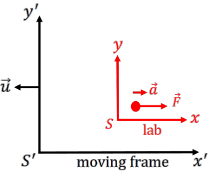
Figure 8.1 show a particle starting from rest and moving under a constant force $F$ in a laboratory. This particle will have a constant acceleration $a$ due to this force. The work done to move this particle from point $x_{1}$ to $x_{2}$ in the laboratory frame $(S)$ is simply $W_{S}= F\Delta x = \Delta K$ because all the motion is in 1-D.

Now, consider what an observer in a moving frame, $S^{\prime }$ would measure for the work done by that force. Here, $S^{\prime }$ is moving at a constant velocity and is also an inertial frame. Because $S^{\prime }$ is moving at a constant velocity, the observer in $S^{\prime }$ would find the same acceleration as the observer in $S$ (e.g., $\frac{\mathrm{d}}{\mathrm{d}t} (v + v_{0}) = \frac{\mathrm{d}v}{\mathrm{d}t}$ ). As a result, both the acceleration and force are unchanged in the moving frame. So

with the same value of $a$ for both frames.

If the force is constant (given in the question), then the work in the moving frame is $W_{S^{\prime }}= \vec{F}\Delta \vec{x}_{S^{\prime }}$, where $\Delta \vec{x}_{S^{\prime }}$ is the displacement in the moving frame. Note that since the motion still takes place in 1-D we can drop vectors (if there are more dimensions, you just need to break up the movement by each coordinate).

For the displacement, $\Delta \vec{x}_{S^{\prime }}$, we need to know how far the particle travels in time $\Delta t$. For a system with constant acceleration (see Chapters 1 and 2), the displacement $\Delta x = \frac{1}{2} at^{2}+v_{i}t$, where $v_{i}$ is the initial velocity of the system. While the particle is initially at rest in the stationary frame, from the perspective of the moving frame, the particle does not start stationary. The moving frame has a velocity of $-u\hat{\imath}$ relative to the lab frame. That means that the moving frame would see the particle as having an initial speed of $u\hat{\imath}$. So we can say that $v_{i}= u$ and the displacement is:

Taking our equations for $F$ and $\Delta x$ in the moving frame, the work done by the force is

where $K_{f}$ is the final kinetic energy and $K_{i}$ in the initial kinetic energy.

So while the values of $W$ and $K$ as measured in the two frames (stationary and moving) may be different, the requirement that $\Delta W = \Delta K$ holds in both frames. Again, this is only the case for inertial frames. In non-inertial frames (e.g., rotating or accelerating frames), the net force will include fictitious forces due to the non-inertial frame and the measured accelerations would be different (see Chapters 4 and 5).

8.4 Gravity¶

8.4.1 Simple Approximation¶

Near the Earth’s surface, we often describe the gravitational force as $\vec{F}_{g}= m\vec{g}$, where $\vec{g}$ is a constant vector that points down vertically and has a constant magnitude.

Consider the case where the position of a heavy box of mass $m$ changes $y_{1}$ to $y_{2}$ in vertical height and that both positions $y_{2}$ and $y_{1}$ are near the Earth’s surface. Work is done by gravity as the box moves by this displacement. The vector describing the displacement of

the box is $\Delta \vec{y} = (y_{2}-y_{1})\hat{\jmath}$ , whereas the gravitational force is $\vec{F}_{g}= -mg\hat{\jmath}$ , which is constant. Taking the equation for work with a constant force, the work is:

Remember, this is the work done by gravity. So if a box is lifted upward $(y_{2}> y_{1})$, gravity acts against the displacement and $W < 0$. If the box is lowered $(y_{2}< y_{1})$, gravity acts with (helps) the displacement and $W > 0$. And if $y_{2}= y_{1}$ then $W$ = 0 (no work is done by gravity).

8.4.2 General Equation¶

In general, the true form of the gravitational force is:

where $G$ is the gravitational constant of $6.67 \times 10^{-11}$ N $\mathrm{m}^{2}\mathrm{kg}^{-2}, M$ is the mass of the object producing the gravitational field, $m$ is the mass of an object being accelerated in the gravitational field, and $r$ is the distance between the centers of the two objects. Thus, the true form for the acceleration due to gravity is given by:

Note that the acceleration due to gravity always points toward the centre of the source of the gravitational field (points radially inward).

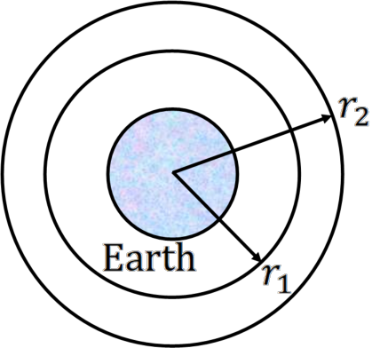
The force of gravity is a radial force with no azimuthal (angle) dependence. That means that any point that has the same radial distance $(|\vec{r}|)$ will have the same magnitude of gravity $|\vec{g}|$. We often describe gravity as a gravitational field, a sphere of influence where any object with a mass $m$ will be subjected to a gravitational force. The magnitude of the gravitational field changes as a function of radial distance. For example, Figure 8.2 shows a cartoon of the Earth with two different vectors, $\vec{r}_{1}$ and $\vec{r}_{2}$. Their magnitudes of gravitational acceleration are:

Since $r_{2}> r_{1}, |\vec{g}_{1}| > |\vec{g}_{2}|$. But any point on a sphere with radius $r_{1}$ around the Earth will have the same magnitude of acceleration due to gravity (e.g., the circles in Figure 8.2), and likewise for all the points on a sphere with radius $r_{2}$. You can think of gravity as a sphere of influence, where any point that has the same distance from the centre of the Earth has the same magnitude of $|\vec{g}|$.

Note that the direction of gravity will be different depending on where you are, because the force always points inward toward the centre of the Earth (in its true form, gravity is not vertical, but radial). For very small distances and positions near the Earth’s surface, you can still assume a vertical direction and constant magnitude for a frame at that surface.

What is the work done by gravity using this general equation?

Well, consider going from $r_{1}$ to $r_{2}$ as shown in Figure 8.2.

Note that if $r_{2}> r_{1}, W < 0$ as we would expect (e.g., you are doing work against gravity to move an object further away). You may recognize $- \frac{GMm}{r}$ as the gravitational potential energy. We will discuss potential energies in more detail in Section 8.6.

8.4.3 Escape velocity¶

The gravitational force follows an inverse square ( $\frac{1}{r^{2}})$ law. So at very large distances from the source of the gravitational field, the gravitational force goes to zero and the work necessary to move a particle also goes to zero (if there is no force, there is no work).

Consider an object that is on the surface of Earth and is launched so that it reaches a very large distance away (assume infinity). Due to Earth’s gravitational field, the object will feel a force that opposes its motion to leave. Gravity will be doing negative work and the kinetic energy of the object will decrease. What speed is needed for this object to just reach infinity? Assume Earth’s atmosphere does not affect its motion.

To solve this problem, we will use the work-kinetic energy theorem (Equation (8.3)).

We just solved for the work to move an object between two radii in a gravitational field. We start with Earth’s surface $(r_{1}= R_{E})$ and we end very far away $(r_{2}= \infty)$. That means that:

where $R_{E}$ is the radius of the Earth, $M_{E}$ is the mass of the Earth, and $m$ is the mass of our object being moved. For kinetic energy, $v_{2}$ = 0 because the object just reaches infinity. As such:

Equation 8.9 describes the escape velocity and for Earth, which is roughly 11 km $\mathrm{s}^{-1}$. The escape velocity is the minimum speed for rockets and satellites to leave Earth’s surface and travel great distances away.

Note that an object starting from rest at a great distance from the Earth will hit the Earth at a speed equivalent to the escape velocity. This converse situation is true because gravity is a conservative force, which we will discuss in the next section.

8.5 Conservative Forces¶

Conservative forces are a class of forces that depend only on position. These forces are also ones where energy is conserved. Common examples of conservative forces are gravity, the spring force, and the electric force. Conservative forces must meet the following criteria:

1. A conservative force does no total work on an object during a round trip.

2. The work done by a conservative force is independent of the path taken between two points.

The first requirement states:

where $\oint$ indicates an integral over a closed loop. For example, if you measure the work between $r_{1}\rightarrow r_{2}$ and then $r_{2}\rightarrow r_{1}$, the work function would be:

For a conservative force, that equation would equal zero.

Now consider the case of gravity,

If you add those two segments, you indeed get $W$ = 0. This is true for any number of stops in the closed loop. As long as your starting and final positions are the same, you will get $W$ = 0 for a conservative force.

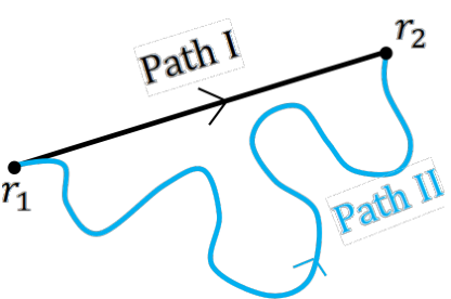
The second requirement states that the total work done to move an object between two points only depends on the initial and final positions. How you get from point one to point two doesn’t matter. Figure 8.3 shows two paths that connect points $r_{1}$ and $r_{2}$. The work done by a conservative force will be the same no matter the path chosen.

And of course, if you go from $r_{1}$ to $r_{2}$ and then from $r_{2}$ back to $r_{1}$, the total work is zero (first criterion) no matter which path you take in either case (e.g., Path I from $r_{1}$ to $r_{2}$ and then Path II from $r_{2}$ back to $r_{1})$.

Note that forces like friction are not conservative forces. First, friction doesn’t depend on position. Second, friction removes energy from a system. Third, the work done by friction in a closed loop is not zero. For example, consider a hockey puck moving in a circle of radius $R$ on a rough horizontal surface that has friction. The friction force on the hockey puck is $\vec{f} = \mu _{K}mg\hat{\theta}$ , and the puck moves so that it is always antiparallel $(180^{\circ})$ to the displacement. So $W_{f}= -f\Delta d = -\mu _{K}mg(2\pi R)$ for a closed loop. Thus, $W_{f}\not =$ 0.

8.5.1 Identifying Conservative Forces¶

A conservative force can be identified mathematically using the following condition:

Note that $\vec{\nabla} \times \vec{F}$ is a vector cross product called the curl of the vector $\vec{F}$ . The $\vec{\nabla}$ symbol is a vector differential operator sometimes called the del or nabla operator. In Cartesian coordinates, it has the form of:

where $\partial$ indicates the partial derivative. For partial derivatives, you ignore any other variable. For example, $\frac{\partial}{\partial x} f(y)$ = 0 because $x$ is not present in the function (you treat $y$ as a constant for a partial derivative with respect to $x)$. For $\vec{\nabla}$ in other coordinate systems, see Appendix A.5.

The curl of $\vec{A}$ (in Cartesian coordinates) is then given by the following matrix.

A conservative force has $\vec{\nabla} \times \vec{F}$ = 0 by definition. We will discuss why in Chapter 8.6.

8.5.2 Example Conservative Forces¶

8.6 Potential Energy¶

The potential energy represents the energy of a system based on its position or configuration. It represents the capacity of the system to do work,

where $\Delta W_{con}$ is the work done by a conservative force. More formally,

Potential energy is associated with conservative forces only. Consider a heavy box. If you lift that box upward, the work done by gravity is negative (gravity opposes the motion), but you increase the potential energy of the box because work is being done against gravity $(W < 0)$. If you lower that box or let go, then gravity is doing positive work on the box $(W > 0)$ and it will have a decrease in potential energy.

Let’s look at the gravitational potential energy between positions $r_{1}$ and $r_{2}$.

In general, the gravitational potential energy is measured between two points. It is a relative energy. You will want to set a convenient reference point. For example, we can set $r_{1}= \infty$, where there would be no contribution from the force, such that:

For gravity problems near Earth’s surface, setting $U$ = 0 at the surface is often convenient.

The potential energy for the spring force going from $x_{1}$ to $x_{2}$ is:

Once again, we want to set a convenient initial value like $x_{1}$ = 0 (the equilibrium position), so that the potential energy of a spring is simply $U = \frac{1}{2} kx^{2}$ relative to that point.

8.7 Conservation of Energy¶

The work-kinetic energy theorem states that $\Delta W = \Delta K$. That is, the total work on a system by a force is equal to the change in the kinetic energy. The total work is the sum of work by conservative forces $(\Delta W_{con})$ and the work by non-conservative forces $(\Delta W_{nc})$:

Setting $\Delta W_{nc}= \Delta E$, or the change in mechanical energy (non-conservative work), we get:

For small times d$t$, you can say that d$E = \mathrm{d}(K+U)$. Integrating these functions then gives

In the absence of non-conservative forces (e.g., if all forces acting on a system are conservative), then $\Delta W_{nc}$ = 0 and $\Delta E$ = 0 such that we get $\Delta (K + U)$ = 0 or $K + U$ = constant. This is the conservation of energy. When energy is conserved, $\Delta K = -\Delta U$ or the change in kinetic energy directly corresponds to a change in potential energy. If kinetic energy increases, then potential energy decreases and vice versa.

8.8 Application of Potential Energy¶

A conservative force can also be written in terms of the potential energy,

for Cartesian coordinates (see Appendix A.5 for other coordinate systems). The $\vec{\nabla}$ operator in this context means the gradient of $U$.

We can use this definition of a conservative force to show that $U(r_{1}\rightarrow r_{2}) = -W(r_{1}\rightarrow r_{2})$.

Exactly as we expect. Thus, the potential energy of a conservative force satisfies $\vec{F} = -\vec{\nabla}U$.

Moreover, $\vec{\nabla} \times \vec{F}$ = 0 for a conservative force. We can substitute in $\vec{F} = -\vec{\nabla}U$,

Note for the above we are assuming that $U$ is twice continuously differentiable. If $U$ can be differentiated twice, then its partial derivatives are independent of the order and all terms cancel (e.g, $\frac{\partial ^{2}U}{\partial y\partial z} = \frac{\partial ^{2}U}{\partial z\partial y})$.

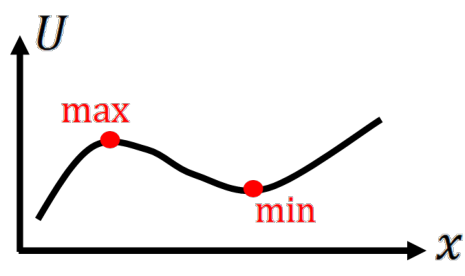
For a potential, $U$, there can be points where $-\vec{\nabla}U = \vec{F}$ = 0. Mathematically, these points are located where the derivative of the potential is zero and correspond to points of local maxima or local minima. Figure 8.5) shows a sketch of a potential with a local maximum and local minimum. These locations are also known as equilibrium points or saddle points.

A local minimum is a stable equilibrium point. At the minimum, if a particle is slightly perturbed, it wouldn’t really go anywhere. The particle will feel a force that just brings it back to the minimum saddle point. Recall that the force is the negative derivative of the potential, so if you perturb the particle to a lower $x$ value, the potential has a negative slope and the force will be positive back toward the saddle point. And if you perturb the particle to a higher $x$ value, the potential has a positive slope and the force will be negative back toward the saddle point. So for a small shift in position, your particle more or less stays at the saddle point.

At the local maximum saddle point, however, a slight perturbation will have a huge effect on the particle’s motion. If you slightly perturb the particle to a lower $x$ value, the potential has a positive slope so the force will be negative toward even more negative $x$ values. (Similar case if you perturb the particle to a higher $x$ value). So a slight perturbation at the maximum of a potential will cause the system to be unstable and move away from that position.

8.9 Summary¶

8.10 Practice Problems¶

See Appendix C for answers to the practice problems.