12. The Lagrange Method August 20, 2025
In this chapter, we will introduce the Lagrangian and the Euler-Lagrange method to solving physics problems. This technique represents another tool in your physics toolkit, much like how we can use energy conservation, momentum conservation, and Newton’s laws to solve physics problems.
12.1 Introduction to the Lagrangian Method ¶ Consider the case of a single particle being acted on by a conservative force in 1-D ( x − (x- ( x −
F = − ∂ U ∂ x F = - \frac{\partial U}{\partial x} F = − ∂ x ∂ U But from Newton’s laws, we can also write the force as
F = d p d t = m d v d t = m d x ˙ d t F = \frac{\mathrm{d}p}{\mathrm{d}t} = m \frac{\mathrm{d}v}{\mathrm{d}t} = m \frac{\mathrm{d}\dot{x}}{\mathrm{d}t} F = d t d p = m d t d v = m d t d x ˙ for constant mass. We can therefore relate the force to the kinetic energy, because the kinetic energy depends on the velocity, K = 1 2 m x ˙ 2 K = \frac{1}{2} m\dot{x}^{2} K = 2 1 m x ˙ 2
d K d x ˙ = m x ˙ , d d t ( d K d x ˙ ) = m d x ˙ d t = F . \frac{\mathrm{d}K}{\mathrm{d}\dot{x}}=m\dot{x},
\qquad
\frac{\mathrm{d}}{\mathrm{d}t}\left(\frac{\mathrm{d}K}{\mathrm{d}\dot{x}}\right)
=m\frac{\mathrm{d}\dot{x}}{\mathrm{d}t}=F. d x ˙ d K = m x ˙ , d t d ( d x ˙ d K ) = m d t d x ˙ = F . We can combine these two force equations to say that:
d d t ( d K d x ˙ ) = − d U d x \frac{\mathrm{d}}{\mathrm{d}t} \Bigg(\frac{\mathrm{d}K}{\mathrm{d}\dot{x}} \Bigg) = - \frac{\mathrm{d}U}{\mathrm{d}x} d t d ( d x ˙ d K ) = − d x d U The above equation is a function of the kinetic and potential energies. So we define the Lagrangian as:
where L L L L L L L L L
L L L L = L ( x , x ˙ L = L(x,\dot{x} L = L ( x , x ˙ K = K ( x ˙ K = K(\dot{x} K = K ( x ˙ U = U ( x ) U = U(x) U = U ( x ) K K K U U U
∂ L ∂ x = − ∂ U ∂ x \frac{\partial L}{\partial x} = - \frac{\partial U}{\partial x} ∂ x ∂ L = − ∂ x ∂ U ∂ L ∂ x ˙ = ∂ K ∂ x ˙ \frac{\partial L}{\partial \dot{x}} = \frac{\partial K}{\partial \dot{x}} ∂ x ˙ ∂ L = ∂ x ˙ ∂ K where ∂ \partial ∂
Therefore, we can rewrite
d d t ( d K d x ˙ ) = − d U d x \frac{\mathrm{d}}{\mathrm{d}t}\left(\frac{\mathrm{d}K}{\mathrm{d}\dot{x}}\right)=-\frac{\mathrm{d}U}{\mathrm{d}x} d t d ( d x ˙ d K ) = − d x d U
d d t ( ∂ L ∂ x ˙ ) = ∂ L ∂ x \frac{\mathrm{d}}{\mathrm{d}t} \Bigg(\frac{\partial L}{\partial \dot{x}} \Bigg) = \frac{\partial L}{\partial x} d t d ( ∂ x ˙ ∂ L ) = ∂ x ∂ L This is the Euler-Lagrange equation . The above example is for 1-D motion in the x − x- x −
d d t ( ∂ L ∂ x ˙ i ) = ∂ L ∂ x i \frac{\mathrm{d}}{\mathrm{d}t} \Bigg(\frac{\partial L}{\partial \dot{x}_{i}} \Bigg) = \frac{\partial L}{\partial x_{i}} d t d ( ∂ x ˙ i ∂ L ) = ∂ x i ∂ L where x i x_{i} x i x , y , r x, y, r x , y , r
The Lagrangian method represents yet another way you can solve problems in physics. For the rest of the chapter, we will look at a few examples.
Show that the units of the Euler-Lagrange equation match expectations.
Show that you get comparable equations for the y y y z z z
12.2 Application to 1-D Problems ¶ Consider a horizontal spring-mass system on a frictionless surface. Compare the differential equation of motion for the mass using (1) Newton’s Laws, (2) Energy Conservation, and (3) the Euler-Lagrange method.
Figure 12.1: Horizontal spring mass system with the spring constant k k k m m m
Solution
Method 1: Newton’s Laws:
∑ F ⃗ = m a ⃗ \sum \vec{F} = m\vec{a} ∑ F = m a − k x = m d 2 x d t 2 = m x ¨ = ⇒ n e t f o r c e i s s p r i n g f o r c e 0 = x ¨ + k m x \begin{aligned}
-kx &= m \frac{\mathrm{d}^{2}x}{\mathrm{d}t^{2}} = m\ddot{x} =\Rightarrow \mathrm{net} \mathrm{force} \mathrm{is} \mathrm{spring} \mathrm{force} \\
0 &= \ddot{x} + \frac{k}{m} x
\end{aligned} − k x 0 = m d t 2 d 2 x = m x ¨ =⇒ net force is spring force = x ¨ + m k x Method 2: Energy Conservation:
E = K + U = ⇒ a s s u m e U = 0 a t e q u i l i b r i u m E = 1 2 m x ˙ 2 + 1 2 k x 2 = ⇒ K = 1 2 m x ˙ 2 , U = 1 2 k x 2 d E d t = d d t ( 1 2 m x ˙ 2 + 1 2 k x 2 ) 0 = m x ˙ d x ˙ d t + k x x ˙ = ⇒ s e t d E d t = 0 0 = x ¨ + k m x = ⇒ s i m p l i f y \begin{aligned}
E &= K + U =\Rightarrow \mathrm{assume} U = 0 \mathrm{at} \mathrm{equilibrium} \\
E &= \frac{1}{2} m\dot{x}^{2}+ \frac{1}{2} kx^{2}=\Rightarrow K = \frac{1}{2} m\dot{x}^{2}, U = \frac{1}{2} kx^{2} \\
\frac{\mathrm{d}E}{\mathrm{d}t} &= \frac{\mathrm{d}}{\mathrm{d}t} \bigg(\frac{1}{2} m\dot{x}^{2}+ \frac{1}{2} kx^{2}\bigg) \\
0 &= m\dot{x} \frac{\mathrm{d}\dot{x}}{\mathrm{d}t} + kx\dot{x} =\Rightarrow \mathrm{set} \frac{\mathrm{d}E}{\mathrm{d}t} = 0 \\
0 &= \ddot{x} + \frac{k}{m} x =\Rightarrow \mathrm{simplify}
\end{aligned} E E d t d E 0 0 = K + U =⇒ assume U = 0 at equilibrium = 2 1 m x ˙ 2 + 2 1 k x 2 =⇒ K = 2 1 m x ˙ 2 , U = 2 1 k x 2 = d t d ( 2 1 m x ˙ 2 + 2 1 k x 2 ) = m x ˙ d t d x ˙ + k x x ˙ =⇒ set d t d E = 0 = x ¨ + m k x =⇒ simplify Method 3: Euler-Lagrange:
For this method, we will solve
d d t ( ∂ L ∂ x ˙ ) = ∂ L ∂ x \frac{\mathrm{d}}{\mathrm{d}t} \Bigg(\frac{\partial L}{\partial \dot{x}} \Bigg) = \frac{\partial L}{\partial x} d t d ( ∂ x ˙ ∂ L ) = ∂ x ∂ L where we can use the energy terms from previously to solve the Lagrangian,
L = K − U = 1 2 m x ˙ 2 − 1 2 k x 2 L = K - U = \frac{1}{2} m\dot{x}^{2}- \frac{1}{2} kx^{2} L = K − U = 2 1 m x ˙ 2 − 2 1 k x 2 Taking each partial differential term of the Euler-Lagrange equations separately:
∂ L ∂ x = ∂ ∂ x ( − 1 2 k x 2 ) = − k x \frac{\partial L}{\partial x} = \frac{\partial}{\partial x} \bigg(- \frac{1}{2} kx^{2}\bigg) = -kx ∂ x ∂ L = ∂ x ∂ ( − 2 1 k x 2 ) = − k x d d t ( ∂ L ∂ x ˙ ) = d d t ( ∂ ∂ x ˙ [ 1 2 m x ˙ 2 ] ) = d d t ( m x ˙ ) = m x ¨ \frac{\mathrm{d}}{\mathrm{d}t} \Bigg(\frac{\partial L}{\partial \dot{x}} \Bigg) = \frac{\mathrm{d}}{\mathrm{d}t} \Bigg(\frac{\partial}{\partial \dot{x}} \bigg[\frac{1}{2} m\dot{x}^{2}\bigg]\Bigg) = \frac{\mathrm{d}}{\mathrm{d}t} (m\dot{x}) = m\ddot{x} d t d ( ∂ x ˙ ∂ L ) = d t d ( ∂ x ˙ ∂ [ 2 1 m x ˙ 2 ] ) = d t d ( m x ˙ ) = m x ¨ So now going back to the Euler-Lagrange equation:
d d t ( ∂ L ∂ x ˙ ) = ∂ L ∂ x \frac{\mathrm{d}}{\mathrm{d}t} \Bigg(\frac{\partial L}{\partial \dot{x}} \Bigg) = \frac{\partial L}{\partial x} d t d ( ∂ x ˙ ∂ L ) = ∂ x ∂ L m x ¨ = − k x 0 = x ¨ + k m x \begin{aligned}
m\ddot{x} &= -kx \\
0 &= \ddot{x} + \frac{k}{m} x
\end{aligned} m x ¨ 0 = − k x = x ¨ + m k x All three methods match!
Use the Lagrangian to get the equation of motion for a vertical mass-spring system and a simple pendulum. Compare to using the other methods.
Thinking about a variable and its time derivative as two separate variables is a little strange to begin with, but if you’re able to set up the Lagrangian system properly, a couple of quick derivatives can get you to the solution a lot faster. It might help your first few tries at it to back out of dot notation very briefly: x x x v v v x x x x ˙ \dot{x} x ˙
m 1 a = ( m 1 + m 2 ) v 2 + m 1 g x 1 + m 2 g ( h − x 1 ) m_{1}a = (m_{1}+ m_{2})v^{2}+ m_{1}gx_{1}+ m_{2}g(h - x_{1}) m 1 a = ( m 1 + m 2 ) v 2 + m 1 g x 1 + m 2 g ( h − x 1 ) from
m 1 x ¨ = ( m 1 + m 2 ) x ˙ + m 1 g x 1 + m 2 g ( h − x 1 ) m_{1}\ddot{x} = (m1 + m2)\dot{x} + m_{1}gx_{1}+ m_{2}g(h - x_{1}) m 1 x ¨ = ( m 1 + m 2 ) x ˙ + m 1 g x 1 + m 2 g ( h − x 1 ) until you get used to the process and so can be easier to see position and velocity as separate variables.
Consider an Atwood machine with a pulley that is a solid disk of mass M M M R ( I = 1 2 M R 2 ) R (I = \frac{1}{2} MR^{2}) R ( I = 2 1 M R 2 ) m 1 m_{1} m 1 m 2 m_{2} m 2 What is the acceleration of m 1 m_{1} m 1 ?
Figure 12.2: The Atwood machine for this problem.
Solution
We’ve looked at this problem previously with energy conservation (Sample Problem 9-3 Figure 12.3 y y y U U U
Figure 12.3: The Atwood machine with the positions of each mass.
For this system, we have:
U = − m 1 g y 1 − m 2 g y 2 K = 1 2 m 1 ( y ˙ 1 ) 2 + 1 2 m 2 ( y ˙ 2 ) 2 + 1 2 I ω 2 \begin{aligned}
U &= -m_{1}gy_{1}- m_{2}gy_{2} \\
K &= \frac{1}{2} m_{1}(\dot{y}_{1})^{2}+ \frac{1}{2} m_{2}(\dot{y}_{2})^{2}+ \frac{1}{2} I\omega ^{2}
\end{aligned} U K = − m 1 g y 1 − m 2 g y 2 = 2 1 m 1 ( y ˙ 1 ) 2 + 2 1 m 2 ( y ˙ 2 ) 2 + 2 1 I ω 2 At first glance, this may seem like a 2-D problem, but the positions of y 1 y_{1} y 1 y 2 y_{2} y 2
(does not stretch) and has a constant length. If the length of the rope is A A A y 1 + y 2 = A y_{1}+ y_{2}= A y 1 + y 2 = A y 2 y_{2} y 2 y ˙ 2 \dot{y}_{2} y ˙ 2 y 1 y_{1} y 1
y 2 = A − y 1 y_{2}= A - y_{1} y 2 = A − y 1 y ˙ 2 = − y ˙ 1 \dot{y}_{2}= -\dot{y}_{1} y ˙ 2 = − y ˙ 1 Moreover, since this is an ideal pulley, it rotates without slipping so we can also use ∣ y ˙ 1 ∣ = R ω |\dot{y}_{1}| = R\omega ∣ y ˙ 1 ∣ = R ω
U = − m 1 g y 1 − m 2 g ( A − y 1 ) U = -m_{1}gy_{1}- m_{2}g(A - y_{1}) U = − m 1 g y 1 − m 2 g ( A − y 1 ) K = 1 2 ( m 1 + m 2 ) ( y ˙ 1 ) 2 + 1 2 I ( y ˙ 1 R ) 2 = 1 2 ( m 1 + m 2 + 1 2 M ) y ˙ 1 2 = ⇒ s u b i n I = 1 2 M R 2 \begin{aligned}
K &= \frac{1}{2} (m_{1}+ m_{2})(\dot{y}_{1})^{2}+ \frac{1}{2} I \bigg(\frac{\dot{y}_{1}}{R} \bigg)^{2} \\
&= \frac{1}{2} \bigg(m_{1}+ m_{2}+ \frac{1}{2} M\bigg)\dot{y}_{1}^{2}=\Rightarrow \mathrm{sub} \mathrm{in} I = \frac{1}{2} MR^{2}
\end{aligned} K = 2 1 ( m 1 + m 2 ) ( y ˙ 1 ) 2 + 2 1 I ( R y ˙ 1 ) 2 = 2 1 ( m 1 + m 2 + 2 1 M ) y ˙ 1 2 =⇒ sub in I = 2 1 M R 2 The Lagrangian (in terms of y 1 y_{1} y 1 y ˙ 1 \dot{y}_{1} y ˙ 1
L = 1 2 ( m 1 + m 2 + 1 2 M ) y ˙ 1 2 + m 1 g y 1 + m 2 g ( A − y 1 ) = 1 2 ( m 1 + m 2 + 1 2 M ) y ˙ 1 2 + ( m 1 − m 2 ) g y 1 + m 2 g A \begin{aligned}
L &= \frac{1}{2} \bigg(m_{1}+ m_{2}+ \frac{1}{2} M\bigg)\dot{y}_{1}^{2}+ m_{1}gy_{1}+ m_{2}g(A - y_{1}) \\
&= \frac{1}{2} \bigg(m_{1}+ m_{2}+ \frac{1}{2} M\bigg)\dot{y}_{1}^{2}+ (m_{1}- m_{2})gy_{1}+ m_{2}gA
\end{aligned} L = 2 1 ( m 1 + m 2 + 2 1 M ) y ˙ 1 2 + m 1 g y 1 + m 2 g ( A − y 1 ) = 2 1 ( m 1 + m 2 + 2 1 M ) y ˙ 1 2 + ( m 1 − m 2 ) g y 1 + m 2 g A Note that this Lagrangian contains a constant term ( m 2 g A ) (m_{2}gA) ( m 2 g A )
The terms of the Euler-Lagrange equation are:
∂ L ∂ y 1 = ∂ ∂ y 1 [ ( m 1 − m 2 ) g y 1 ] = ( m 1 − m 2 ) g \frac{\partial L}{\partial y_{1}} = \frac{\partial}{\partial y_{1}} [(m_{1}- m_{2})gy_{1}] = (m_{1}- m_{2})g ∂ y 1 ∂ L = ∂ y 1 ∂ [( m 1 − m 2 ) g y 1 ] = ( m 1 − m 2 ) g d d t ( ∂ L ∂ y ˙ 1 ) = d d t ( ∂ ∂ y ˙ 1 [ 1 2 ( m 1 + m 2 + 1 2 M ) y ˙ 1 2 ] ) \frac{\mathrm{d}}{\mathrm{d}t} \Bigg(\frac{\partial L}{\partial \dot{y}_{1}} \Bigg) = \frac{\mathrm{d}}{\mathrm{d}t} \Bigg(\frac{\partial}{\partial \dot{y}_{1}} \bigg[\frac{1}{2} \bigg(m_{1}+ m_{2}+ \frac{1}{2} M\bigg)\dot{y}_{1}^{2}\bigg]\Bigg) d t d ( ∂ y ˙ 1 ∂ L ) = d t d ( ∂ y ˙ 1 ∂ [ 2 1 ( m 1 + m 2 + 2 1 M ) y ˙ 1 2 ] ) = d d t [ ( m 1 + m 2 + 1 2 M ) y ˙ 1 ] = ( m 1 + m 2 + 1 2 M ) y ¨ 1 \begin{aligned}
&= \frac{\mathrm{d}}{\mathrm{d}t} \bigg[\bigg(m_{1}+ m_{2}+ \frac{1}{2} M\bigg)\dot{y}_{1}\bigg] \\
&= \bigg(m_{1}+ m_{2}+ \frac{1}{2} M\bigg)\ddot{y}_{1}
\end{aligned} = d t d [ ( m 1 + m 2 + 2 1 M ) y ˙ 1 ] = ( m 1 + m 2 + 2 1 M ) y ¨ 1 And the Euler-Lagrange equation is:
12.3 Application in 2-D ¶ Consider an object of mass m m m Solve the Euler-Lagrange equations for this object.
Solution
For this problem we have motion in 2-D because the object is in an elliptical orbit, which means that
v ⃗ = v r r ^ + v θ θ ^ = r ˙ r ^ + ( r θ ˙ ) θ ^ \vec{v} = v_{r}\hat{r} + v_{\theta}\hat{\theta} = \dot{r}\hat{r} + (r\dot{\theta})\hat{\theta} v = v r r ^ + v θ θ ^ = r ˙ r ^ + ( r θ ˙ ) θ ^ where r ^ \hat{r} r ^ θ ^ \hat{\theta} θ ^
To solve the Lagrangian, we need the sources of potential and kinetic energy. The only source of potential energy is the gravitational field and the only source of kinetic energy is the orbital motion (note that we are using the central force potential, not the effective potential here). For this system, we have:
U = − G M m r K = 1 2 m v 2 \begin{aligned}
U &= - \frac{GMm}{r} \\
K &= \frac{1}{2} mv^{2}
\end{aligned} U K = − r GM m = 2 1 m v 2 where the squared velocity is given by:
v 2 = v r 2 + v θ 2 = r ˙ 2 + ( r θ ˙ ) 2 v^{2}= v_{r}^{2}+ v_{\theta}^{2}= \dot{r}^{2}+ (r\dot{\theta})^{2} v 2 = v r 2 + v θ 2 = r ˙ 2 + ( r θ ˙ ) 2 See Chapter 1.2
U = − G M m r K = 1 2 m ( r ˙ 2 + r 2 θ ˙ 2 ) \begin{aligned}
U &= - \frac{GMm}{r} \\
K &= \frac{1}{2} m(\dot{r}^{2}+ r^{2}\dot{\theta}^{2})
\end{aligned} U K = − r GM m = 2 1 m ( r ˙ 2 + r 2 θ ˙ 2 ) And the Lagrangian is:
L = 1 2 m ( r ˙ 2 + r 2 θ ˙ 2 ) + G M m r L = \frac{1}{2} m(\dot{r}^{2}+ r^{2}\dot{\theta}^{2}) + \frac{GMm}{r} L = 2 1 m ( r ˙ 2 + r 2 θ ˙ 2 ) + r GM m So the Lagrangian is really L = L ( r , r ˙ , θ , θ ˙ L = L(r,\dot{r},\theta,\dot{\theta} L = L ( r , r ˙ , θ , θ ˙
∂ L ∂ r = d d t ( ∂ L ∂ r ˙ ) \frac{\partial L}{\partial r} = \frac{\mathrm{d}}{\mathrm{d}t} \Bigg(\frac{\partial L}{\partial \dot{r}} \Bigg) ∂ r ∂ L = d t d ( ∂ r ˙ ∂ L ) ∂ L ∂ θ = d d t ( ∂ L ∂ θ ˙ ) \frac{\partial L}{\partial \theta} = \frac{\mathrm{d}}{\mathrm{d}t} \Bigg(\frac{\partial L}{\partial \dot{\theta}} \Bigg) ∂ θ ∂ L = d t d ( ∂ θ ˙ ∂ L ) Note, however, that the Lagrangian does not have any θ \theta θ
∂ L ∂ θ = 0 \frac{\partial L}{\partial \theta} = 0 ∂ θ ∂ L = 0 Thus, from the Euler-Lagrange equation:
∂ L ∂ θ = d d t ( ∂ L ∂ θ ˙ ) \frac{\partial L}{\partial \theta} = \frac{\mathrm{d}}{\mathrm{d}t} \Bigg(\frac{\partial L}{\partial \dot{\theta}} \Bigg) ∂ θ ∂ L = d t d ( ∂ θ ˙ ∂ L ) 0 = d d t ( ∂ L ∂ θ ˙ ) 0 = \frac{\mathrm{d}}{\mathrm{d}t} \Bigg(\frac{\partial L}{\partial \dot{\theta}} \Bigg) 0 = d t d ( ∂ θ ˙ ∂ L ) So the derivative of the Lagrangian with angular velocity ( ∂ L ∂ θ ˙ (\frac{\partial L}{\partial \dot{\theta}} ( ∂ θ ˙ ∂ L
∂ L ∂ θ ˙ = ∂ ∂ θ ˙ ( 1 2 m r 2 θ ˙ 2 ) = m r 2 θ ˙ = c o n s t a n t \frac{\partial L}{\partial \dot{\theta}} = \frac{\partial}{\partial \dot{\theta}} \bigg(\frac{1}{2} mr^{2}\dot{\theta}^{2}\bigg) = mr^{2}\dot{\theta} = \mathrm{constant} ∂ θ ˙ ∂ L = ∂ θ ˙ ∂ ( 2 1 m r 2 θ ˙ 2 ) = m r 2 θ ˙ = constant The term m r 2 θ ˙ mr^{2}\dot{\theta} m r 2 θ ˙ Chapter 6 Chapter 10
Now let’s look at the radial terms.
∂ L ∂ r = ∂ ∂ r ( 1 2 m r 2 θ ˙ 2 + G M m r ) = m r θ ˙ 2 − G M m r 2 \frac{\partial L}{\partial r} = \frac{\partial}{\partial r} \bigg(\frac{1}{2} mr^{2}\dot{\theta}^{2}+ \frac{GMm}{r} \bigg) = mr\dot{\theta}^{2}- \frac{GMm}{r^{2}} ∂ r ∂ L = ∂ r ∂ ( 2 1 m r 2 θ ˙ 2 + r GM m ) = m r θ ˙ 2 − r 2 GM m d d t ( ∂ L ∂ r ˙ ) = d d t ( ∂ ∂ r ˙ [ 1 2 m r ˙ 2 ] ) = d d t ( m r ˙ ) = m r ¨ \frac{\mathrm{d}}{\mathrm{d}t} \Bigg(\frac{\partial L}{\partial \dot{r}} \Bigg) = \frac{\mathrm{d}}{\mathrm{d}t} \Bigg(\frac{\partial}{\partial \dot{r}} \bigg[\frac{1}{2} m\dot{r}^{2}\bigg]\Bigg) = \frac{\mathrm{d}}{\mathrm{d}t} (m\dot{r}) = m\ddot{r} d t d ( ∂ r ˙ ∂ L ) = d t d ( ∂ r ˙ ∂ [ 2 1 m r ˙ 2 ] ) = d t d ( m r ˙ ) = m r ¨ And the Euler-Lagrange equation is:
∂ L ∂ r = d d t ( ∂ L ∂ r ˙ ) \frac{\partial L}{\partial r} = \frac{\mathrm{d}}{\mathrm{d}t} \Bigg(\frac{\partial L}{\partial \dot{r}} \Bigg) ∂ r ∂ L = d t d ( ∂ r ˙ ∂ L ) m r θ ˙ 2 − G M m r 2 = m r ¨ mr\dot{\theta}^{2}- \frac{GMm}{r^{2}} = m\ddot{r} m r θ ˙ 2 − r 2 GM m = m r ¨ At this point, we have two equations of motion.
L = m r 2 θ ˙ = ⇒ L L = mr^{2}\dot{\theta} =\Rightarrow L L = m r 2 θ ˙ =⇒ L
m r ¨ = m r θ ˙ 2 − G M m r 2 (the radial component) m\ddot{r}=mr\dot{\theta}^2-\frac{GMm}{r^2}
\qquad\text{(the radial component)} m r ¨ = m r θ ˙ 2 − r 2 GM m (the radial component) We can combine these equations to remove the θ ˙ \dot{\theta} θ ˙
m r ¨ = m r L 2 m 2 r 4 − G M m r 2 = ⇒ θ ˙ = L m r 2 r ¨ = L 2 m 2 r 3 − G M r 2 \begin{aligned}
m\ddot{r} &= mr \frac{L^{2}}{m^{2}r^{4}} - \frac{GMm}{r^{2}} =\Rightarrow \dot{\theta} = \frac{L}{mr^{2}} \\
\ddot{r} &= \frac{L^{2}}{m^{2}r^{3}} - \frac{GM}{r^{2}}
\end{aligned} m r ¨ r ¨ = m r m 2 r 4 L 2 − r 2 GM m =⇒ θ ˙ = m r 2 L = m 2 r 3 L 2 − r 2 GM We have now created a 1-D equation of motion because L , G , m L, G, m L , G , m M M M r r r
You will also notice that this is the effective force for a system moving under a gravitational force that we found in Chapter 10.6 Chapter 11
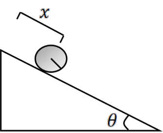
12.4 Example Problem: Sphere on an Incline ¶ The following problem includes rolling and translation motion.
Figure 12.4: A sphere of radius R R R θ \theta θ
Solution
First, we need the potential and kinetic energies. The only source of potential energy is the change in gravitational potential energy as the sphere rolls down. For kinetic energy, we have the translation and rotation of the sphere.
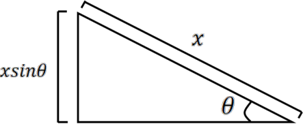
Since the motion is along the incline only, we will define x ^ \hat{x} x ^ U U U x x x Figure 12.5 x x x x x x x sin θ x\sin \theta x sin θ
Figure 12.5: Using Pythagorean theorem we can determine the change in height of the sphere.
The potential energy is therefore:
U = − M g Δ h U = -Mg\Delta h U = − M g Δ h U = − M g x sin θ U = -Mgx\sin \theta U = − M gx sin θ The potential energy is negative because U U U x x x
For the kinetic energy, we have the translation and rotation motion of the sphere, which we defined in Chapter 8
K = 1 2 M x ˙ 2 + 1 2 I ω 2 K = \frac{1}{2} M\dot{x}^{2}+ \frac{1}{2} I\omega ^{2} K = 2 1 M x ˙ 2 + 2 1 I ω 2 For a sphere, I = 2 5 M R 2 I = \frac{2}{5} MR^{2} I = 5 2 M R 2 Appendix A.4
ω = v c m R = x ˙ R \omega = \frac{v_{cm}}{R} = \frac{\dot{x}}{R} ω = R v c m = R x ˙ Substituting the moment of inertia equation and the rolling without slipping condition, the kinetic energy becomes:
K = 1 2 M x ˙ 2 + 1 2 ( 2 5 ) M R 2 ( x ˙ R ) 2 = 7 10 M x ˙ 2 K = \frac{1}{2} M\dot{x}^{2}+ \frac{1}{2} \bigg(\frac{2}{5} \bigg)MR^{2}\bigg(\frac{\dot{x}}{R} \bigg)^{2}= \frac{7}{10} M\dot{x}^{2} K = 2 1 M x ˙ 2 + 2 1 ( 5 2 ) M R 2 ( R x ˙ ) 2 = 10 7 M x ˙ 2 Now we can solve for the Lagrangian:
L = K − U = 7 10 M x ˙ 2 + M g x sin θ L = K - U = \frac{7}{10} M\dot{x}^{2}+ Mgx\sin \theta L = K − U = 10 7 M x ˙ 2 + M gx sin θ Note that θ \theta θ x ^ \hat{x} x ^
The Euler-Lagrange equations are:
∂ L ∂ x = M g sin θ \frac{\partial L}{\partial x} = Mg\sin \theta ∂ x ∂ L = M g sin θ d d t ( ∂ L ∂ x ˙ ) = d d t ( 7 5 M x ˙ ) = 7 5 M x ¨ \frac{\mathrm{d}}{\mathrm{d}t} \Bigg(\frac{\partial L}{\partial \dot{x}} \Bigg) = \frac{\mathrm{d}}{\mathrm{d}t} \bigg(\frac{7}{5} M\dot{x}\bigg) = \frac{7}{5} M\ddot{x} d t d ( ∂ x ˙ ∂ L ) = d t d ( 5 7 M x ˙ ) = 5 7 M x ¨ To solve for the motion itself, we equate the two Euler-Lagrange equations:
d d t ( ∂ L ∂ x ˙ ) = ∂ L ∂ x 7 5 M x ¨ = M g sin θ x ¨ = 5 7 g sin θ \begin{aligned}
\frac{\mathrm{d}}{\mathrm{d}t} \Bigg(\frac{\partial L}{\partial \dot{x}} \Bigg) &= \frac{\partial L}{\partial x} \\
\frac{7}{5} M\ddot{x} &= Mg\sin \theta \\
\ddot{x} &= \frac{5}{7} g\sin \theta
\end{aligned} d t d ( ∂ x ˙ ∂ L ) 5 7 M x ¨ x ¨ = ∂ x ∂ L = M g sin θ = 7 5 g sin θ Thus, our acceleration is proportional to gravity, with a sin θ \sin\theta sin θ 5 / 7 5/7 5/7
12.5 Challenging Problem: Particle on a Wire ¶ For this problem, the solution is not a simple differential equation. Consider whether you would try to solve this problem using Newton’s Laws or energy conservation.
A particle of mass m m m y = a x 4 y = ax^{4} y = a x 4 What is the equation of motion for the particle?
Figure 12.6: The function y = a x 4 y = ax^{4} y = a x 4 m m m
Solution
To help solve this problem, we will break it down into a few parts. We will get the equation of motion when we have expressions for K K K U U U
a) What is the velocity of the particle?
Since the particle moves in two-dimensions, x x x y y y
v ⃗ = x ˙ ı ^ + y ˙ ȷ ^ \vec{v} = \dot{x}\hat{\imath} + \dot{y}\hat{\jmath} v = x ˙ ^ + y ˙ ^ The position in the y-direction can be described by the equation of the wire, y = a x 4 y = ax^{4} y = a x 4 y ˙ = 4 a x 3 x ˙ \dot{y} = 4ax^{3}\dot{x} y ˙ = 4 a x 3 x ˙
v ⃗ = x ˙ ı ^ + 4 a x 3 x ˙ ȷ ^ \vec{v} = \dot{x}\hat{\imath} + 4ax^{3}\dot{x}\hat{\jmath} v = x ˙ ^ + 4 a x 3 x ˙ ^ b) Solve the Lagrangian.
We know that,
so let’s find our kinetic and potential energies. We only have translation kinetic energy from the motion of the particle,
K = 1 2 m v 2 K = \frac{1}{2} mv^{2} K = 2 1 m v 2 where,
v 2 = v ⃗ ⋅ v ⃗ v^{2}= \vec{v} \cdot \vec{v} v 2 = v ⋅ v v 2 = x ˙ 2 + y ˙ 2 v^{2}= \dot{x}^{2}+ \dot{y}^{2} v 2 = x ˙ 2 + y ˙ 2 v 2 = x ˙ 2 + ( 4 a x 3 x ˙ ) 2 v^{2}= \dot{x}^{2}+ (4ax^{3}\dot{x})^{2} v 2 = x ˙ 2 + ( 4 a x 3 x ˙ ) 2 v 2 = x ˙ 2 + 16 a 2 x 6 x ˙ 2 v^{2}= \dot{x}^{2}+ 16a^{2}x^{6}\dot{x}^{2} v 2 = x ˙ 2 + 16 a 2 x 6 x ˙ 2 v 2 = x ˙ 2 ( 1 + 16 a 2 x 6 ) v^{2}= \dot{x}^{2}(1 + 16a^{2}x^{6}) v 2 = x ˙ 2 ( 1 + 16 a 2 x 6 ) Therefore, we can solve for the kinetic energy in terms of x x x x ˙ \dot{x} x ˙
K = 1 2 m x ˙ 2 ( 1 + 16 a 2 x 6 ) K = \frac{1}{2} m\dot{x}^{2}(1 + 16a^{2}x^{6}) K = 2 1 m x ˙ 2 ( 1 + 16 a 2 x 6 ) The only source of potential energy is gravity,
U = m g h w h e r e h = y U = mgh \qquad \mathrm{where}\ h = y U = m g h where h = y U = m g y w h e r e U = 0 w h e n y = 0 U = mgy \qquad \mathrm{where}\ U = 0\ \mathrm{when}\ y = 0 U = m g y where U = 0 when y = 0 U = m g a x 4 U = mgax^{4} U = m g a x 4 Note that U U U y y y U > 0 U > 0 U > 0
L = K − U L = 1 2 m x ˙ 2 ( 1 + 16 a 2 x 6 ) − m g a x 4 \begin{aligned}
L &= K - U \\
L &= \frac{1}{2} m\dot{x}^{2}(1 + 16a^{2}x^{6}) - mgax^{4}
\end{aligned} L L = K − U = 2 1 m x ˙ 2 ( 1 + 16 a 2 x 6 ) − m g a x 4 c) Find the differential equation of motion of the bead.
To do this let’s solve the Euler-Lagrange equation:
d d t ( ∂ L ∂ x ˙ ) = ∂ L ∂ x \frac{\mathrm{d}}{\mathrm{d}t} \Bigg(\frac{\partial L}{\partial \dot{x}} \Bigg) = \frac{\partial L}{\partial x} d t d ( ∂ x ˙ ∂ L ) = ∂ x ∂ L We can start by solving the left-side:
∂ L ∂ x = ∂ ∂ x [ 1 2 m x ˙ 2 ( 1 + 16 a 2 x 6 ) − m g a x 4 ] ∂ L ∂ x = 1 2 m x ˙ 2 [ 16 a 2 ( 6 x 5 ) ] − 4 m g a x 3 ∂ L ∂ x = 48 m x ˙ 2 a 2 x 5 − 4 m g a x 3 \begin{aligned}
\frac{\partial L}{\partial x} &= \frac{\partial}{\partial x} \bigg[\frac{1}{2} m\dot{x}^{2}(1 + 16a^{2}x^{6}) - mgax^{4}\bigg] \\
\frac{\partial L}{\partial x} &= \frac{1}{2} m\dot{x}^{2}\Big[16a^{2}(6x^{5})\Big] - 4mgax^{3} \\
\frac{\partial L}{\partial x} &= 48m\dot{x}^{2}a^{2}x^{5}- 4mgax^{3}
\end{aligned} ∂ x ∂ L ∂ x ∂ L ∂ x ∂ L = ∂ x ∂ [ 2 1 m x ˙ 2 ( 1 + 16 a 2 x 6 ) − m g a x 4 ] = 2 1 m x ˙ 2 [ 16 a 2 ( 6 x 5 ) ] − 4 m g a x 3 = 48 m x ˙ 2 a 2 x 5 − 4 m g a x 3 Now let’s solve the right-side:
∂ L ∂ x ˙ = ∂ ∂ x ˙ [ 1 2 m x ˙ 2 ( 1 + 16 a 2 x 6 ) − m g a x 4 ] = m x ˙ ( 1 + 16 a 2 x 6 ) , d d t ( ∂ L ∂ x ˙ ) = d d t [ m x ˙ ( 1 + 16 a 2 x 6 ) ] . \begin{aligned}
\frac{\partial L}{\partial\dot{x}}
&=\frac{\partial}{\partial\dot{x}}
\left[\frac12m\dot{x}^2(1+16a^2x^6)-mgax^4\right]\\
&=m\dot{x}(1+16a^2x^6),\\
\frac{\mathrm{d}}{\mathrm{d}t}\left(\frac{\partial L}{\partial\dot{x}}\right)
&=\frac{\mathrm{d}}{\mathrm{d}t}\left[m\dot{x}(1+16a^2x^6)\right].
\end{aligned} ∂ x ˙ ∂ L d t d ( ∂ x ˙ ∂ L ) = ∂ x ˙ ∂ [ 2 1 m x ˙ 2 ( 1 + 16 a 2 x 6 ) − m g a x 4 ] = m x ˙ ( 1 + 16 a 2 x 6 ) , = d t d [ m x ˙ ( 1 + 16 a 2 x 6 ) ] . d d t ( ∂ L ∂ x ˙ ) = m x ¨ ( 1 + 16 a 2 x 6 ) + m x ˙ ( 96 a 2 x 5 x ˙ ) \frac{\mathrm{d}}{\mathrm{d}t} \Bigg(\frac{\partial L}{\partial \dot{x}} \Bigg) = m\ddot{x}(1 + 16a^{2}x^{6}) + m\dot{x}(96a^{2}x^{5}\dot{x}) d t d ( ∂ x ˙ ∂ L ) = m x ¨ ( 1 + 16 a 2 x 6 ) + m x ˙ ( 96 a 2 x 5 x ˙ ) Now we can equate the two sides and solve for the differential equation of motion:
d d t ( ∂ L ∂ x ˙ ) = ∂ L ∂ x \frac{\mathrm{d}}{\mathrm{d}t} \Bigg(\frac{\partial L}{\partial \dot{x}} \Bigg) = \frac{\partial L}{\partial x} d t d ( ∂ x ˙ ∂ L ) = ∂ x ∂ L m x ¨ ( 1 + 16 a 2 x 6 ) + m x ˙ ( 96 a 2 x 5 x ˙ ) = 48 m x ˙ 2 a 2 x 5 − 4 m g a x 3 m\ddot{x}(1 + 16a^{2}x^{6}) + m\dot{x}(96a^{2}x^{5}\dot{x}) = 48m\dot{x}^{2}a^{2}x^{5}- 4mgax^{3} m x ¨ ( 1 + 16 a 2 x 6 ) + m x ˙ ( 96 a 2 x 5 x ˙ ) = 48 m x ˙ 2 a 2 x 5 − 4 m g a x 3 m x ¨ ( 1 + 16 a 2 x 6 ) + m x ˙ ( 4 8 2 x 5 x ˙ ) + 4 m g a x 3 = 0 m\ddot{x}(1 + 16a^{2}x^{6}) + m\dot{x}(48^{2}x^{5}\dot{x}) + 4mgax^{3}= 0 m x ¨ ( 1 + 16 a 2 x 6 ) + m x ˙ ( 4 8 2 x 5 x ˙ ) + 4 m g a x 3 = 0 x ¨ ( 1 + 16 a 2 x 6 ) + x ˙ ( 4 8 2 x 5 x ˙ ) + 4 g a x 3 = 0 \ddot{x}(1 + 16a^{2}x^{6}) + \dot{x}(48^{2}x^{5}\dot{x}) + 4gax^{3}= 0 x ¨ ( 1 + 16 a 2 x 6 ) + x ˙ ( 4 8 2 x 5 x ˙ ) + 4 g a x 3 = 0 The solution is a differential equation of motion, but it is difficult to solve because it is non-linear with respect to both x x x x ˙ \dot{x} x ˙
Try solving this problem using energy conservation. Hint: Remember that energy conservation uses full derivatives and not partial derivatives.
If you were to try Newton’s law, to solve this problem, what other force is acting on the bead other than gravity (it is this force that makes applying Newton’s laws difficult)?
12.6 Real-World Applications ¶ Initially, it might seem like the Euler-Lagrange Method is unnecessarily complicated, but we’re really just touching the edge of what it can be used for. Remember that this textbooks is still mostly focusing on simple, idealized problems. The real world of experimentation and research is much more complex, and many physics problems don’t have simple, analytical solutions and can only be probed numerically using computers.
Lagrangian mechanics help simplify the calculations for complex or even chaotic systems where forces are hard to define or the initial conditions can drastically change the outcome (e.g., consider the motion of a double pendulum
One common application of Lagrangian mechanics is with magnetohydrodynamics (MHD), which is the study of fluids that conduct electrically. MHD is used in many branches of physics, but one example is nuclear fusion experimentation, where many experiments seek to produce energy by magnetically confining a fast-moving plasma in a torus. MHD research must solving various equations such as the equation of state, mass continuity, Faraday’s law, and Ohm’s law simultaneously for the entire system, and these equations are usually non-linear with time. As such, Lagrangian mechanics are often employed to simplify the problem.
For more information: Wikipedia webpage on MHD , listing various forms and equations. Science article
12.7 Summary on the Lagrange Method ¶ We have shown that the Lagrange method involves two main steps. First, you define the Lagrangian:
Second, you solve the Euler-Lagrange equations. For example, for motion in the x − x- x −
d d t ( ∂ L ∂ x ˙ ) = ∂ L ∂ x \frac{\mathrm{d}}{\mathrm{d}t} \Bigg(\frac{\partial L}{\partial \dot{x}} \Bigg) = \frac{\partial L}{\partial x} d t d ( ∂ x ˙ ∂ L ) = ∂ x ∂ L The Euler-Lagrange equations and the Lagrangian hold under very general circumstances. You can apply these equations to n-dimensional systems (e.g., you do not need to be restricted to 3 dimensions). Systems in n-dimension are often called Euclidean space. In broad terms, you can express the Euler-Lagrange equations as:
d d t ( ∂ L ∂ x ˙ i ) = ∂ L ∂ x i \frac{\mathrm{d}}{\mathrm{d}t} \Bigg(\frac{\partial L}{\partial \dot{x}_{i}} \Bigg) = \frac{\partial L}{\partial x_{i}} d t d ( ∂ x ˙ i ∂ L ) = ∂ x i ∂ L where x i x_{i} x i
Strategies for employing the Lagrange method successfully .
Choose your coordinate system carefully. You want a coordinate system that simplifies the problem.
Write out K K K U U U L = K − U L = K -U L = K − U L = K − U L = K -U L = K − U
Solve the Euler-Lagrange equations for each coordinate system separately. Note that a constant in the potential (e.g., U → U ( x i ) + U 0 ) U \rightarrow U(x_{i}) + U_{0}) U → U ( x i ) + U 0 )
If L L L x i x_i x i ∂ L / ∂ x i = 0 \partial L/\partial x_i=0 ∂ L / ∂ x i = 0 ∂ L / ∂ x ˙ i \partial L/\partial\dot{x}_i ∂ L / ∂ x ˙ i Section 12.3
Once you have L L L
12.8 Practice Problems ¶ See Appendix C for answers to the practice problems.
An ideal string is wrapped around a disk of mass M M M R R R 1 2 M R 2 \frac{1}{2} MR^{2} 2 1 M R 2 U U U y y y
Figure 12.7: Figure for Problem 12-4
Two identical blocks of mass m m m U U U
A block of mass m m m k k k x x x
a) What is the kinetic energy of the mass?
b) What is the potential energy of the mass?
c) Find the Lagrangian of the system and solve the Euler-Lagrange equations.
Figure 12.8: Figure for Problem 12-6
A circular disk of mass M M M R R R s = R / 2 s = R/2 s = R /2
a) What is the Lagrangian for this system?
b) Check that this answer makes sense by applying the Euler-Lagrange equations and showing that you get a standard differential equation of motion.
Figure 12.10: Figure for Problem 12-8
A snowboarder of mass m m m
x = a 4 ( 2 θ + sin 2 θ ) y = a 4 ( 1 − cos 2 θ ) \begin{aligned}
x &= \frac{a}{4} (2\theta + \sin 2\theta) \\
y &= \frac{a}{4} (1 - \cos 2\theta)
\end{aligned} x y = 4 a ( 2 θ + sin 2 θ ) = 4 a ( 1 − cos 2 θ ) where a a a < θ < π < \theta < \pi < θ < π
a) If gravity is the only force on the snowboarder, find the potential energy. Express this in terms of θ \theta θ θ ˙ \dot{\theta} θ ˙
b) What is the kinetic energy of the snowboarder? Express this in terms of θ \theta θ θ ˙ \dot{\theta} θ ˙
c) What is the Lagrangian of the system? Express this in terms of θ \theta θ θ ˙ \dot{\theta} θ ˙
d) Use the Euler-Lagrange equations to find the differential equation of motion. Do not solve this equation.
See the figure below. A mass M M M
a) Describe how the system would move if it is displaced a small distance x x x θ \theta θ
b) What is the potential energy of this system?
c) What is the kinetic energy of this system?
d) Use the Lagrange method to find the differential equation of motion for this system? Note: you must solve the x x x θ \theta θ
Figure 12.12: Figure for Problem 12-10