10. Central Forces and Motion in Space

In this chapter, we will expand on a few concepts that have already been covered. We will discuss central forces and their application. We will also expand on the motion of objects in 3-D under central forces and apply the concepts of central forces to gravity.

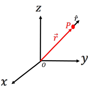
10.1 Introduction to Central Forces¶

Consider a particle of fixed mass at a position that can be defined by the vector $\vec{r}$ with respect to an origin. We’ll also define $\hat{r}$ as the unit vector in the direction of $\vec{r}$ . Recall that a unit vector has a length of one such that $\hat{r} \cdot \hat{r}$ = 1 and $\vec{r} = r\hat{r}$ .

Figure shows the point P in standard 3D Cartesian coordinates. — Figure 10.1:Point $P$ is the particle. Shown in red is the vector $\vec{r}$ in the figure to the right. $\hat{r}$ is shown in black as the unit vector in the direction of $\vec{r}$ .

A central force is defined as follows:

The force is directed toward or away from the origin (e.g., the force acts along $\hat{r}$ )
The magnitude of the force depends only on the distance $r$ .

\vec{F} = f(r)\hat{r} = f(r) \frac{\vec{r}}{r}

(1)

A central force is attractive if $f(r) < 0$ (the force points toward the origin) and repulsive if $f(r) > 0$ (the force points away from the origin). An attractive force acts to bring the particle to the origin, whereas a repulsive force acts to move the particle away from the origin. We have already discussed several such central forces in previous chapters.

Examples of central forces:

Gravity: $\vec{F}=-\dfrac{GMm}{r^2}\hat{r}$

Electrostatic force: $\vec{F}=\dfrac{kQq}{r^2}\hat{r}$

Spring Force: $\vec{F} = -kr\hat{r} =\Rightarrow$ often written in terms of 1-D motion (e.g., $F = -kx)$

Note that gravity and the spring force are always attractive $(f(r) < 0)$ . The electrostatic force can be either attractive or repulsive (depends on the charges).

10.2 Properties of Central Forces¶

10.2.1 Central Forces are Conservative Forces¶

Central forces are all conservative forces. In Chapter 8, we discussed conservative forces and showed that conservative forces obey,

\vec{\nabla} \times \vec{F} = 0

(2)

If a central force is defined as $\vec{F} = f(r)\hat{r}$ , then we can show that $\vec{\nabla} \times \vec{F}$ = 0 for all central forces. For simplicity, we will use spherical coordinates for the curl (see Appendix A.5).

\begin{aligned} \vec{\nabla} \times \vec{F} &= \frac{1}{r^{2}\sin \theta} \begin{vmatrix} \hat{r} & r\hat{\theta} & r\sin\theta\,\hat{\varphi} \\ \dfrac{\partial}{\partial r} & \dfrac{\partial}{\partial \theta} & \dfrac{\partial}{\partial \varphi} \\ f(r) & 0 & 0 \end{vmatrix} \\ &= \frac{1}{r^{2}\sin \theta}(0 - 0)\hat{r} + \frac{1}{r\sin \theta}\left(\frac{\partial f(r)}{\partial \varphi} - 0\right)\hat{\theta} + \frac{1}{r}\left(0 - \frac{\partial f(r)}{\partial \theta}\right)\hat{\varphi} \\ &= 0 \end{aligned}

(3)

Because $f(r)$ does not depend on $\theta$ or $\varphi$ (by definition), the partial derivatives of $f(r)$ with $\theta$ and $\varphi$ equal zero and the curl of $\vec{F}$ is zero. This means a general central force will always be conservative. Note that a conservative force may not be central. The force must still obey the two criteria in the first section to be defined as a central force.

If a central force is conservative, that means there is a potential field $U(r)$ that can describe the force where,

U = -\int f(r)\mathrm{d}r

(4)

where d $r$ is a tiny path. Recall that for conservative fields, the change in potential energy is independent of the path. Only the initial and final points matter.

Or we can solve for the force if we know the potential of the central force:

\vec{F} = -\vec{\nabla}U = - \frac{\partial U}{\partial r} \hat{r}

(5)

since the force is radial, only the radial component of the gradient matters. For a review of the properties of conservative forces, see Chapter 8.

10.2.2 Angular Momentum is Conserved¶

Another feature of central forces is that angular momentum is conserved. The angular momentum for a particle is defined as:

\vec{L} = \vec{r} \times \vec{p}

(6)

where $\vec{r}$ is the radial vector from the origin to the particle and $\vec{p} = m\vec{v}$ is the momentum of that particle. If the mass of the particle is constant, the time derivative of the angular momentum is then:

\begin{aligned} \frac{\mathrm{d}\vec{L}}{\mathrm{d}t} &= \frac{\mathrm{d}}{\mathrm{d}t} (\vec{r} \times \vec{p}) \\ &= \frac{\mathrm{d}\vec{r}}{\mathrm{d}t} \times \vec{p} + \vec{r} \times \frac{\mathrm{d}\vec{p}}{\mathrm{d}t} \\ &= \vec{v} \times \vec{p} + \vec{r} \times \vec{F} =\Rightarrow \vec{v} = \frac{\mathrm{d}\vec{r}}{\mathrm{d}t} \mathrm{and} \vec{F} = \frac{\mathrm{d}\vec{p}}{\mathrm{d}t} \\ &= \vec{v} \times (m\vec{v}) + \vec{r} \times (f(r)\hat{r}) =\Rightarrow \mathrm{for} \mathrm{a} \mathrm{central} \mathrm{force}, \vec{F} = f(r)\hat{r} \end{aligned}

(7)

=m\underbrace{(\vec{v}\times\vec{v})}_{0} +f(r)\underbrace{(\vec{r}\times\hat{r})}_{0}=0,

(8)

= 0

(9)

So for any central force with $\vec{F} = f(r)\hat{r}$ , the angular momentum of the system is conserved (assuming constant mass).

10.2.3 Motion will occur on a plane¶

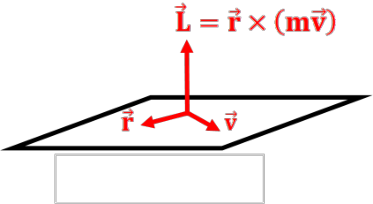
The motion of a particle under the action of a central force will take place on a 2-D plane even if the particle’s position is defined in a 3-D coordinate system. Figure 10.2 shows a vector diagram of the angular momentum. The angular momentum is defined as the vector cross product of $\vec{r} \times \vec{p} = m(\vec{r} \times \vec{v})$ . That means that the angular momentum vector is perpendicular to both the radial vector and the velocity vector (see diagram).

Figure shows the angular momentum vector pointing away from a plane defined by the radial and velocity vectors. — Figure 10.2:Vector diagram for the angular momentum, $\vec{L}$ . Recall that $\vec{L} = \vec{r}\times (m\vec{v})$ and will therefore be perpendicular to both $\vec{r}$ and $\vec{v}$ .

In the previous section, we showed that the angular momentum is constant under a central force. That includes both magnitude and direction. Since $\vec{L}$ defines the normal that is perpendicular to the plane given by $\vec{r}$ and $\vec{v}$ , that plane must also be constant (otherwise the direction of $\vec{L}$ would change). So both the radius and velocity vectors are confined and motion will only occur on this 2-D plane (e.g., the plane in Figure 10.2).

10.3 Equation of Motion for a Central Force¶

Since motion under a central force occurs on a 2-D plane (see Chapter 10.2.3), we can simplify the motion of a particle under a central force. It is generally convenient to use polar coordinates (see Chapter 1.2).

A central force has the form of $\vec{F} = f(r)\hat{r}$ . If this is the only force acting on a particle, then we can also use Newton’s second law to say that $\vec{F} = m\vec{a}$ (for a constant particle mass). Thus, we can say that $f(r)\hat{r} = m\vec{a}$ .

In polar coordinates, $\vec{a}$ is written as:

\vec{a} = \underbrace{(\ddot{r} - \dot{\theta}^{2}r)}_{a_{r}}\hat{r}+\underbrace{(2\dot{\theta}\dot{r} + \ddot{\theta}r)}_{a_{\theta}}\hat{\theta}

(10)

where we have a radial component of the acceleration and a tangential component (azimuthal or $\theta$ component). But the central force is radial only. This is a definition of a central force. As a consequence, we can make two conclusions about the acceleration.

1) The radial acceleration is $m\vec{a}_{r}= f(r)\hat{r}$ because both act in the radial direction.

f(r)\hat{r} = m\vec{a}_{r}= m(\ddot{r} - \dot{\theta}^{2}r)\hat{r}

(11)

2) The tangential acceleration is $\vec{a}_{\theta}$ = 0 because central forces are only radial in direction. Setting the tangential acceleration component to zero, we get:

\begin{aligned} 0 &= 2\dot{\theta}\dot{r} + \ddot{\theta}r \\ 0 &= \frac{1}{r} \frac{\mathrm{d}}{\mathrm{d}t} (r^{2}\dot{\theta}) \end{aligned}

(12)

where the latter equation can be expanded to recover the $\vec{a}_{\theta}$ terms. Recall that this comes from the definition of the radial vector in polar coordinates (see Chapter 1.2 for a refresher).

In the above equation, we have a time derivative equal to zero. If you have a time derivative equal to zero, that means the term in the derivative is a constant.

r^{2}\dot{\theta} = \mathrm{constant}

(13)

Note that we can also get to the conclusion that $r^{2}\dot{\theta}$ is constant using the angular momentum instead of Newton’s second law. For the angular momentum, we have $\vec{L} = \vec{r}\times \vec{p} = \vec{r}\times (m\vec{v})$ . In polar coordinates, $\vec{v} = \dot{r}\hat{r} + \dot{\theta}r\hat{\theta}$ (Chapter 1.2), so

\vec{L} = (r\hat{r}) \times m(\dot{r}\hat{r} + \dot{\theta}r\hat{\theta})

(14)

=m\dot{r}r\underbrace{(\hat{r}\times\hat{r})}_{0} +m\dot{\theta}r^2(\hat{r}\times\hat{\theta})

(15)

= m\dot{\theta}r^{2}\hat{k} =\Rightarrow \mathrm{for} \mathrm{cylindrical} \mathrm{coordinates}

(16)

Since $\vec{L}$ is a constant, the magnitude of $\vec{L}$ is also a constant. The magnitude of $\vec{L}$ is

|\vec{L}| = m\dot{\theta}r^{2}= \mathrm{constant}

(17)

Since $m$ is also a constant for our particle (assumed), we get that $\dot{\theta}r^{2}$ must be a constant.

10.4 Effective Potential¶

The effective potential is used to simplify complex problems involving central forces. For central forces, the motion occurs in a 2-D plane, so we can use plane polar coordinates to describe the motion. (Note that polar coordinates are convenient because the potential energy for the central force is radial.) In polar coordinates, the energy equations are:

\begin{aligned} U &= -\int \vec{F} \cdot \mathrm{d}\vec{r} = -\int f(r)\mathrm{d}r \\ K &= \frac{1}{2} mv^{2}= \frac{1}{2} m(\dot{r}^{2}+ r^{2}\dot{\theta}^{2}) \end{aligned}

(18)

We can use Equation 10.5 to re-write the kinetic energy in terms of the linear velocity $\dot{r}$

and the angular momentum using $\dot{\theta}=L/(mr^2)$ .

K = \frac{1}{2} m\dot{r}^{2}+ \frac{1}{2} \frac{L^{2}}{mr^{2}}

(19)

The total energy of the system is then:

\begin{aligned} E &= K + U \\ E &= \frac{1}{2} m\dot{r}^{2}+ \frac{1}{2} \frac{L^{2}}{mr^{2}} + U(r) \end{aligned}

(20)

where $U(r)$ represents the potential produced by the central force. The first term depends only on $\dot{r}$ whereas the other two terms depend only on $r$ ( $m$ and $L$ are constant).

E=\underbrace{\frac12m\dot{r}^2}_{\dot{r}\text{ term}} +\underbrace{\frac12\frac{L^2}{mr^2}+U(r)}_{r\text{ terms}}.

(21)

This should look familiar. This is a 1-D energy equation. You have the energy entirely expressed along one coordinate axis. For example, when we looked at a mass and spring, $K = \frac{1}{2} m\dot{x}^{2}$ and $U = \frac{1}{2} kx^{2}$ , such that $E = \frac{1}{2} m\dot{x}^{2}+ \frac{1}{2} kx^{2}$ , all the energy is along one axis $(x)$ . So the energy equation for a central force can be simplified into a 1-D energy equation with an additional $r$ term. By definition, the potential energy will depend on position alone. So we can combine the two $r-$ terms into an effective potential energy, $U_{eff}$ :

U_{eff}= \frac{1}{2} \frac{L^{2}}{mr^{2}} + U(r)

(22)

where first term is related to the angular momentum and is often called the centrifugal potential. The second term is the potential due to the central force itself.

Coming back to our energy equation, we have:

E = \frac{1}{2} m\dot{r}^{2}+ U_{eff}

(23)

Which looks exactly like a 1-D energy problem, even though the system may be in a 3-D space and moving in a 2-D plane. By cutting back on the dimensions, we make the math much easier.

We can re-write Equation 10.9 as follows (solving for $\dot{r}^{2})$ :

\dot{r}^{2}= \frac{2}{m} (E - U_{eff})

(24)

The term $\dot{r}^{2}$ is always positive or zero. So if $\dot{r}^{2}\ge 0$ , then

\begin{aligned} \frac{2}{m} (E - U_{eff}) &\ge 0 \\ E &\ge U_{eff} \end{aligned}

(25)

So with just the effective potential, we can start to get an idea of the allowed properties in the system. The system energy must be at least equal to the effective potential.

Continued

Solution

The energy equation for our central force is $E = \frac{1}{2} m\dot{r}^{2}+U_{eff}$ . If $\dot{r}$ = 0, then $E = U_{eff}$ . The potential of the central force.

\begin{aligned} U(r) &= - f(r)\mathrm{d}r \\ U(r) &= -\int (- \frac{\gamma}{r^{3}})\mathrm{d}r \\ U(r) &= - \frac{\gamma}{2r^{2}} \end{aligned}

(26)

So our effective potential is:

\begin{aligned} U_{eff}&= \frac{1}{2} \frac{L^{2}}{mr^{2}} + U(r) \\ U_{eff}&= \frac{1}{2} \frac{L^{2}}{mr^{2}} - \frac{\gamma}{2r^{2}} \\ U_{eff}&= \frac{1}{2r^{2}} \Bigg(\frac{L^{2}}{m} - \gamma \Bigg) \end{aligned}

(27)

Since $U_{eff}= E$ , we have:

E = \frac{1}{2r^{2}} \Bigg(\frac{L^{2}}{m} - \gamma \Bigg)

(28)

r^{2}= \frac{1}{2E} \Bigg(\frac{L^{2}}{m} - \gamma \Bigg)

(29)

r=\sqrt{\frac{1}{2E}\left(\frac{L^2}{m}-\gamma\right)}.

(30)

We ignore the negative case for the square-root because by definition, $r > 0$ .

As for the kind of motion, this object moves in such a way that $r$ is constant. In other words, the particle is moving in a perfect circle (circular motion).

10.5 Effective Force¶

If you have an effective potential, then you can define an effective force associated with that effective potential. This is not a true force, however. The only true force acting on the system is the central force. We’re just treating the constant angular momentum as an additional potential term and therefore creating an effective “force” that produces it. This is why we use the term “effective”, because it has an effect on the system that represents the motion, but it is not a real force. The effective force is a mathematical construct.

In general, we can get the force from the gradient of a potential, $\vec{F} = -\vec{\nabla}U$ . Since our potential only depends on position $r$ , we only care about the $r$ component of the gradient.

\begin{aligned} \vec{F}_{eff}&= - \frac{\partial U_{eff}}{\partial r} \hat{r} \\ &= - \frac{\partial}{\partial r} \Bigg(\frac{1}{2} \frac{L^{2}}{mr^{2}} + U(r)\Bigg)\hat{r} \end{aligned}

(31)

= -\Bigg(- \frac{L^{2}}{mr^{3}} \Bigg)\hat{r} - \frac{\mathrm{d}U(r)}{\mathrm{d}r} \hat{r}

(32)

= \frac{L^{2}}{mr^{3}} \hat{r} - \frac{\mathrm{d}U(r)}{\mathrm{d}r} \hat{r}

(33)

The effective force has two terms. The first term comes from the angular momentum of the system (the centrifugal potential) and the second term comes from the central force.

Sample Problem 10-2

A modification of Earth’s gravitational field is often described as $U(r)=-\dfrac{\gamma}{r}\left(1+\dfrac{\varepsilon}{r^2}\right)$

where $\gamma$ and $\varepsilon$ are constants. What is the effective force associated with this potential? Assume a particle of mass $m$ and an angular momentum of $L$ .

Solution

The effective force is given by $\vec{F}_{eff}= -\vec{\nabla}U_{eff}$ .

\begin{aligned} \vec{F}_{eff}&= - \frac{\partial U_{eff}}{\partial r} \hat{r} \\ \vec{F}_{eff}&= - \frac{\partial}{\partial r} \Bigg[\frac{1}{2} \frac{L^{2}}{mr^{2}} + U(r)\Bigg]\hat{r} \end{aligned}

(34)

\vec{F}_{eff}= - \frac{\partial}{\partial r} \Bigg[\frac{1}{2} \frac{L^{2}}{mr^{2}} - \frac{\gamma}{r} \bigg(1 + \frac{\varepsilon}{r^{2}} \bigg)\Bigg]\hat{r}

(35)

\vec{F}_{eff}= -\Bigg(- \frac{L^{2}}{mr^{3}} + \frac{\gamma}{r^{2}} + \frac{3\gamma \varepsilon}{r^{4}} \Bigg)\hat{r}

(36)

\vec{F}_{eff}= \Bigg(\frac{L^{2}}{mr^{3}} - \frac{\gamma}{r^{2}} - \frac{3\gamma \varepsilon}{r^{4}} \Bigg)\hat{r}

(37)

10.6 Example: Gravity as a Central Force¶

The gravitational force has the form $f(r)\hat{r}$ and is therefore a central force:

\vec{F} = - \frac{GMm}{r^{2}} \hat{r}

(38)

The gravitational force also falls under a class of forces that are called inverse-square laws. Any force proportional to $r^{-2}$ follows an inverse-square law.

What is the effective potential for a system moving under a gravitational force?

\begin{aligned} U_{eff}&= \frac{1}{2} \frac{L^{2}}{mr^{2}} + U(r) \\ &= \frac{1}{2} \frac{L^{2}}{mr^{2}} - \frac{GMm}{r} \end{aligned}

(39)

Recall that

U(r) = -\int \vec{F} \cdot \mathrm{d}\vec{r} = - \frac{GMm}{r}

(40)

relative to $U$ = 0 at infinity.

1) Consider the case where $L$ = 0**:** $L$ = 0 is a special case where an object has no angular momentum. That means the object only has motion along the radial direction (e.g., recall that $L = m\dot{\theta}r^{2}$ , so if $L$ = 0, then $\dot{\theta}$ = 0 and $\dot{\vec{r}} = \dot{r}\hat{r}$ ).

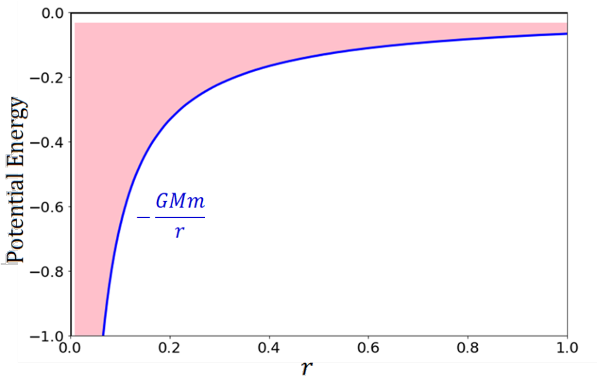
If $L$ = 0, then $U_{eff}= U(r)$ . That is, the effective potential is just the gravitational potential. In terms of the allowed energies, we have:

\begin{aligned} E &= \frac{1}{2} m\dot{r}^{2}- \frac{GMm}{r} \\ E &\ge - \frac{GMm}{r} \end{aligned}

(41)

because $\dot{r}^{2}\ge 0$ .

Figure 10.3 shows the potential energy for an object moving under the gravitational force when $L$ = 0. The blue curve shows $U_{grav}$ and the shaded in area shows the allowed energies, $E > U_{grav}$ . All constants are given arbitrary values for the purposes of plotting. Note that $E$ can be positive, depending on the value of $\dot{r}$ . We can only define the minimum allowed energy at each radius. For the actual motion within this system, we need to solve the equation:

\dot{r}^{2}= \frac{2}{m} \bigg(E + \frac{GMm}{r} \bigg)

(42)

\frac{\mathrm{d}r}{\mathrm{d}t} =\pm\sqrt{\frac{2}{m}\left(E+\frac{GMm}{r}\right)}.

(43)

\frac{\mathrm{d}r}{\sqrt{E+GMm/r}}=\pm\sqrt{\frac{2}{m}}\,\mathrm{d}t.

(44)

If you know the system energy, $E$ , you can then solve for how the position changes with time $r(t)$ by integrating both sides.

Figure 10.3 from the source textbook — Figure 10.3:The allowed energies for a system in a gravitational potential with no angular momentum $(L$ = 0). Blue curve shows the potential from gravity and the shaded in area shows the allowed values of energy.

2) Consider the case where $L \not =$ 0**:** If $L$ is a non-zero, then the system has angular momentum, and that angular momentum is constant. If $L \not =$ 0, then

U_{eff}= \frac{1}{2} \frac{L^{2}}{mr^{2}} - \frac{GMm}{r}

(45)

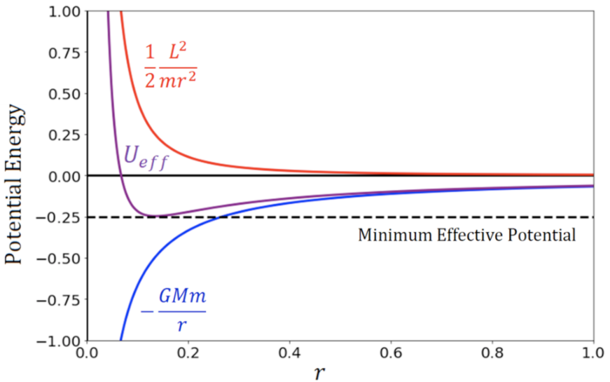
Figure 10.4 shows the effective potential (purple curve) for an object under the potential $U_{eff}$ . The figure compares the effective potential with the centrifugal potential (red curve) and the gravitational potential (blue curve). The constants are given arbitrary values.

The effective potential still sets the minimum value of energy that a system can have. That is, we still have the condition $E \ge U_{eff}$ because $\dot{r}^{2}\ge 0$ . So the effective potential curve $U_{eff}$ in Figure 10.4 shows the minimum allowed energy of the system. Note that this curve has a distinct shape with a local minimum in the potential. This shape has profound impact on how objects in this potential are going to move.

For simplicity, let’s look at the condition where $\dot{r}$ = 0. An object with $\dot{r}$ = 0 has no radial motion. Instead, all the motion will be transverse due to the non-zero angular momentum $(L = m\dot{\theta}r^{2})$ . Note that transverse motion describes rotation. So an object in a gravitational field will rotate or orbit around the source of that gravitational field.

Figure 10.4 from the source textbook — Figure 10.4:The effective potential energy for a system moving in a gravitational field. The effective potential is in purple. The potential from gravity is in blue and the centrifugal potential is in red. The functions use arbitrary constants and units for plotting.

Let’s find the conditions for a stable orbit. We will substitute $\gamma = GMm$ to make the math a bit easier to read. Assuming $\dot{r}$ = 0:

E = U_{eff}

(46)

0 = U_{eff}- E

(47)

\begin{aligned} 0 &= \frac{1}{2} \frac{L^{2}}{mr^{2}} - \frac{\gamma}{r} - E =\Rightarrow U_{eff}= \frac{1}{2} \frac{L^{2}}{mr^{2}} - \frac{\gamma}{r} \\ 0 &= \frac{L^{2}}{m} - 2\gamma r - 2Er^{2}=\Rightarrow \mathrm{multiply} \mathrm{by} 2r^{2} \end{aligned}

(48)

The above equation is a quadratic equation with $r$ , where the solution is:

r=\frac{-(-2\gamma)\pm\sqrt{(-2\gamma)^2-4(-2E)(L^2/m)}}{2(-2E)} =\frac{\gamma\pm\sqrt{\gamma^2+2EL^2/m}}{-2E}.

(49)

where $\gamma = GMm$ .

To have a real orbit, we need to have real values for $r$ . By definition, $r \ge 0$ , or $r$ must be positive. The above equation has two positive (real) solutions for $r$ if $E < 0$ or if the energy is negative.

Let’s consider a few cases.

Case (1) $E = E_{\min}$ : Figure 10.4 shows that there is an energy minimum, $E_{\min}$ . A system with $E = E_{\min}$ is a special case.

First, we need to find the value of $E_{\min}$ . We can do that by finding the position when the potential has a local minimum by taking the derivative of $U_{eff}$ with respect to $r$ .

\begin{aligned} \frac{\mathrm{d}U_{eff}}{\mathrm{d}r} &= 0 \\ 0 &= \frac{\mathrm{d}}{\mathrm{d}r} \Bigg(\frac{1}{2} \frac{L^{2}}{mr^{2}} - \frac{\gamma}{r} \Bigg) \end{aligned}

(50)

\begin{aligned} 0 &= - \frac{L^{2}}{mr^{3}} + \frac{\gamma}{r^{2}} \\ 0 &= - \frac{L^{2}}{m} + \gamma r \\ r_{\min}&= \frac{L^{2}}{\gamma m} \end{aligned}

(51)

The energy at this minimum position is:

\begin{aligned} 0 &= \frac{L^{2}}{m} - 2\gamma r_{\min}- 2E_{\min}r_{\min}^{2} \\ 0 &= \frac{L^{2}}{m} - 2\gamma \Bigg(\frac{L^{2}}{\gamma m} \Bigg) - 2E_{\min}\Bigg(\frac{L^{2}}{\gamma m} \Bigg)^{2} \end{aligned}

(52)

0 = 1 - 2 - 2E_{\min}\Bigg(\frac{L^{2}}{\gamma ^{2}m} \Bigg)

(53)

E_{\min}= - \frac{1}{2} \frac{m\gamma ^{2}}{L^{2}}

(54)

The values of $r_{\min}$ and $E_{\min}$ represent a special case where the is only one unique solution to the quadratic equation. If you sub $E = E_{\min}$ into the quadratic equation for $r$ , you will get that $r = r_{\min}$ as the only solution, as expected.

When $E = E_{\min}$ , it means that your orbital solution has the minimum allowed potential energy and it can only orbit with a single, fixed radius. This solution describes a circular orbit.

Case (2) $E > E_{\min}$ and $E < 0$ : Consider Figure 10.4 for a particle with an energy of $E = -0.2$ . This energy puts the system just above the minimum effective potential curve. With that energy, the allowed radii for the particle are between $r \approx 0.1$ and $r \approx 0.24$ (under

the condition $E \ge U_{eff}$ in Figure 10.4). That is, for radii of $r < 0.1$ and $r > 0.24, E = -0.2$ would be below effective potential curve, which is not allowed.

This scenario describes a bound elliptical orbit. The particle can move freely from $r \approx 0.1$ to $r \approx 0.24$ and back again all with the same energy (energy is conserved). The positions of $r \approx 0.1$ and $r \approx 0.24$ are special, because there are where $\dot{r}$ is instantaneously zero, but in this case, the radial velocity does not stay zero (unlike in Case 1).

Let’s say the particle starts at $t$ = 0 at $r \approx 0.1$ . At this instantaneous moment, $E = U_{eff}$ , so $\dot{r} = 0 (K_{r}$ = 0). But this is an instantaneous moment. The particle is allowed to move to larger radii (given its energy), but $E = K_{r}+U_{eff}$ will still be constant, so as $U_{eff}$ drops toward larger radii, $K_{r}$ will increase. As the particle approaches $r \approx 0.24, E \rightarrow U_{eff}$ and $K_{r}\rightarrow$ 0 again. The particle cannot travel further radially (it does not have enough energy) and instead, it will turn around back toward the origin. Thus, the $r \approx 0.1$ and $r \approx 0.24$ points are the turnaround points in this elliptical orbit. The motion is bounded by these two limits. We’ll discuss elliptical orbits in more detail in Chapter 11.

Case (3) $E > 0$ : If the energy is positive, then the quadratic equation for radius:

r=\frac{\gamma\pm\sqrt{\gamma^2+2EL^2/m}}{-2E}

(55)

will have one positive and one negative solution. Since negative radii are unphysical (by definition), this case describes an unbound orbit. Unbound orbits arise when systems have too much energy to be contained by the gravitational field. We will come back to these orbits in Chapter 11.

Sample Problem 10-3

In Sample Problem 10-2, we used a modification of Earth’s gravitational field described

as $U(r)=-\dfrac{\gamma}{r}\left(1+\dfrac{\varepsilon}{r^2}\right)$ , where $\gamma$ and $\varepsilon$ are constants. A particle of mass $m$ is in a closed

orbit in this gravitational potential with an angular momentum of $L$ . If the angular momentum of the system is the exact value to put the particle in a circular orbit, what are the possible radii for a circular orbit?

Solution

You have a circular orbit when $\mathrm{d}U_{eff}/\mathrm{d}r=0$ . For this system, $U_{eff}=L^2/(2mr^2)+U(r)$ ,

where $U(r)$ is the potential given in the equation. If you plot the effective potential, depending on the constants, you will get a curve that looks like:

Figure 10.5:An example of $U_{eff}$ with arbitrary constants.

So, we see that there are multiple possible places where the derivative of $U_{eff}$ will be zero (local maxima or minima). Note that the exact the shape of the effective potential curve will depend on the constants themselves.

To get the equations for a circular orbit, let’s first solve for the derivative and set that to be zero:

\begin{aligned} \frac{\mathrm{d}U_{eff}}{\mathrm{d}r} &= 0 \\ 0 &= \frac{\mathrm{d}}{\mathrm{d}r} \Bigg[\frac{1}{2} \frac{L^{2}}{mr^{2}} - \frac{\gamma}{r} \bigg(1 + \frac{\varepsilon}{r^{2}} \bigg)\Bigg] \end{aligned}

(56)

\begin{aligned} 0 &= - \frac{L^{2}}{mr^{3}} + \frac{\gamma}{r^{2}} + \frac{3\gamma \varepsilon}{r^{4}} \\ 0 &= - \frac{L^{2}r}{m} + \gamma r^{2}+ 3\gamma \varepsilon =\Rightarrow \mathrm{multiply} \mathrm{by} r^{4} \end{aligned}

(57)

Continued

Let’s use the quadratic equation to solve for $r$ .

r=\frac{-(-L^2/m)\pm\sqrt{(-L^2/m)^2-4(\gamma)(3\gamma\varepsilon)}}{2\gamma}.

(58)

So there are two values of $r > 0$ for which we can have a saddle point in the effective potential.

r=\frac{L^2/m\pm\sqrt{(L^2/m)^2-12\gamma^2\varepsilon}}{2\gamma}.

(59)

Since these are by definition the radii at a local maxima or minima, they are the solutions for a circular orbit. But only a local minimum will produce a stable circular orbit. Recall the discussion on saddle points from Chapter 8.8.

Remember that effective force is the gradient of a potential, so our initial assumption was that $F_{eff}$ = 0 for circular orbits. This means that our two radii are at the minimum and maximum points of potential, one being at a stable position and the other at an unstable position. We can look back to Chapter 8, to the analogy of a ball resting atop the potential energy curve to helped to describe the stability of positions. This means that the radius at the max potential will be unstable and the radius at the minimum potential will be stable.

10.7 Real World Application¶

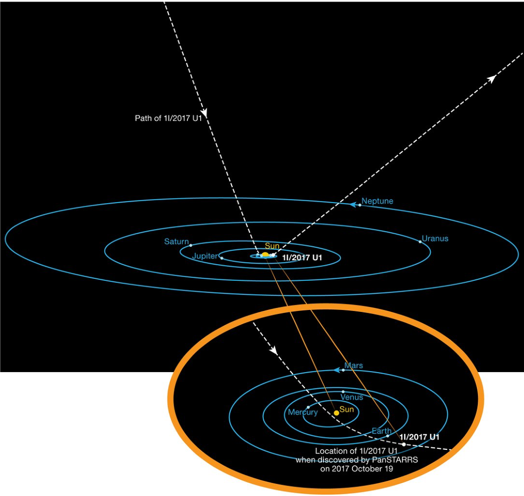
Planets, comets, and asteroids have bound orbits around the Sun. That means, they do not have enough energy to escape the Sun. If an object enters the Solar System with too much energy $(E > 0)$ it will not stick around. That exact event happened with the first-detected interstellar asteroid, ‘Oumuamua.

It was discovered on 19 October 2017 by Robert Weryk (a Canadian) using the University of Hawai‘i Pan-STARRS1 telescope and was noted to be moving very quickly. With more observations, it was found to have an unbound orbit. The figure below shows the orbit of ‘Oumuamua relative to the Solar System planets. The Sun’s gravitational field deflected its motion, but isn’t enough to keep ‘Oumuamua from escaping. This type of orbit is called a hyperbolic orbit (more on this in Chapter 11).

Based on its orbital properties, it was determined that ‘Oumuamua originated from outside the Solar System, making it the first detected asteroid to have come from another star. It was subsequently given the name ‘Oumuamua, which roughly means “first visitor from far away” in Hawaiian. It is also the first entry in a whole new asteroid classification system,

“1I”, where the “I” indicates it’s an interstellar object.

Figure shows the hyperbolic orbit of Oumuamua with a zoomed-out look for the whole Solar System and a zoomed in look with the inner planets. — Figure 10.6:The orbit of ‘Oumuamua. Image credit: ESO.

For more information: NASA’s basic information page on ‘Oumuamua has some good introductory reading plus an animation of the object’s orbit near its closest approach to the Sun and this NASA article highlights how much and how little we know about ‘Oumuamua.

10.8 Summary¶

Key Takeaways

This chapter introduces the central forces, which are a class of conservative forces that only have a radial dependence.

\vec{F} = f(r)\hat{r}

(60)

All motion under a central force takes place in a 2-D plane because these forces also conserve angular momentum

L = m\dot{\theta}r^{2}= \mathrm{constant}

(61)

As a result, the motion of a particle under a central force can be simplified greatly. Since central forces are also conservative forces, they can be described by a potential energy

\vec{F} = -\vec{\nabla}U = - \frac{\partial U}{\partial r} \hat{r}

(62)

which only depends on position.

Using energy conservation, we can also write the kinetic energy in terms of position and a constant angular momentum.

E = \frac{1}{2} m\dot{r}^{2}+ \frac{1}{2} \frac{L^{2}}{mr^{2}} + U(r)

(63)

We define the effective potential as the sum of the centrifugal potential (from angular momentum) and the central force potential,

U_{eff}= \frac{1}{2} \frac{L^{2}}{mr^{2}} + U(r)

(64)

If the central force potential is known, one can predict the motion of objects. Some basic cases are:

$\dot{r}$ = 0: All motion is transverse (azimuthal) and $E = U_{eff}$ .
$L$ = 0: All motion is along $\hat{r}$ and magnitude depends only on distance.
$L \not =$ 0 and $\dot{r} \not =$ 0: There will be a mix of linear and azimuthal motion and $E > U_{eff}$ because $\dot{r}^{2}$ is always positive.

Important Equations

Central Force:

\vec{F}=f(r)\hat{r}=m\vec{a}_r=m(\ddot{r}-\dot{\theta}^2r)\hat{r}

(65)

Potential of a Central Force:

\vec{F}=-\vec{\nabla}U=-\frac{\partial U}{\partial r}\hat{r}

(66)

Constant Angular Momentum:

L = m\dot{\theta}r^{2} = \mathrm{constant}

(67)

Kinetic Energy:

K = \frac{1}{2} m\dot{r}^{2}+ \frac{1}{2} \frac{L^{2}}{mr^{2}}

(68)

Energy:

\begin{aligned} E &= \frac{1}{2} m\dot{r}^{2}+ \frac{1}{2} \frac{L^{2}}{mr^{2}} + U(r) \\ E &= \frac{1}{2} m\dot{r}^{2}+ U_{eff} \end{aligned}

(69)

Effective Potential Energy:

U_{eff}= \frac{1}{2} \frac{L^{2}}{mr^{2}} + U(r)

(70)

Effective Force:

\vec{F}_{eff}= -\vec{\nabla}U_{eff}

(71)

Position of Saddle Point and Minimum Energy for Gravity:

r_{\min}= \frac{L^{2}}{\gamma m}

(72)

E_{\min}= - \frac{1}{2} \frac{m\gamma ^{2}}{L^{2}} \mathrm{for} \gamma = GMm \mathrm{and} U = - \frac{\gamma}{r}

(73)

10.9 Practice Problems¶

See Appendix C for answers to the practice problems.