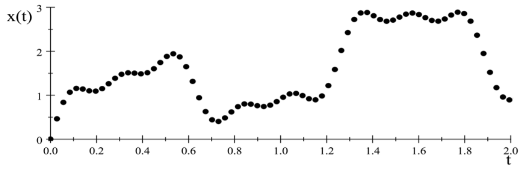
Development of classical mechanics has involved a close and synergistic interweaving of physics and mathematics, that continues to play a key role in these fields. The concepts of scalar and vector fields play a pivotal role in describing the force fields and particle motion in both the Newtonian formulation of classical mechanics and electromagnetism. Thus it is imperative that you be familiar with the sophisticated mathematical formalism used to treat multivariate scalar and vector fields in classical mechanics. Ordinary and partial differential equations up to second order, as well as integration of algebraic and trigonometric functions play a major role in classical mechanics. It is assumed that you already have a working knowledge of differential and integral calculus in sufficient depth to handle this material. Computer codes, such as Mathematica, MatLab, and Maple, or symbolic calculators, can be used to obtain mathematical solutions for complicated cases.
The following 9 appendices provide brief summaries of matrix algebra, vector algebra, orthogonal coordinate systems, coordinate transformations, tensor algebra, multivariate calculus, vector differential plus integral calculus, Fourier analysis and time-sampled waveform analysis. The manipulation of scalar and vector fields is greatly facilitated by transforming to orthogonal curvilinear coordinate systems that match the symmetries of the problem. These appendices discuss how to account for the time dependence of the orthogonal unit vectors for curvilinear coordinate systems. It is assumed that, except for coordinate transformations and tensor algebra, you have been introduced to these topics in linear algebra and other physics courses, and thus the purpose of these appendices is to serve as a reference plus brief review.
Matrix algebra provides an elegant and powerful representation of multivariate operators, and coordinate transformations that feature prominently in classical mechanics. For example they play a pivotal role in finding the eigenvalues and eigenfunctions for coupled equations that occur in rigid-body rotation, and coupled oscillator systems. An understanding of the role of matrix mechanics in classical mechanics facilitates understanding of the equally important role played by matrix mechanics in quantal physics.
It is interesting that although determinants were used by physicists in the late 19th century, and the concept of matrix algebra was developed by Arthur Cayley in England in 1855, many of these ideas were the work of Hamilton, and the discussion of matrix algebra was buried in a more general discussion of determinants. Matrix algebra was an esoteric branch of mathematics, little known by the physics community, until 1925 when Heisenberg proposed his innovative new quantum theory. The striking feature of this new theory was its representation of physical quantities by sets of time-dependent complex numbers and a peculiar multiplication rule. Max Born recognized that Heisenberg’s multiplication rule is just the standard “row times column” multiplication rule of matrix algebra; a topic that he had encountered as a young student in a mathematics course. In 1924 Richard Courant had just completed the first volume of the new text Methods of Mathematical Physics during which Pascual Jordan had served as his young assistant working on matrix manipulation. Fortuitously, Jordan and Born happened to share a carriage on a train to Hanover during which Jordan overheard Born talk about his problems trying to work with matrices. Jordan introduced himself to Born and offered to help. This led to publication, in September 1925, of the famous Born-Jordan paper[Bor25a] that gave the first rigorous formulation of matrix mechanics in physics. This was followed in November by the Born-Heisenberg-Jordan sequel[Bor25b] that established a logical consistent general method for solving matrix mechanics problems plus a connection between the mathematics of matrix mechanics and linear algebra. Matrix algebra developed into an important tool in mathematics and physics during World War 2 and now it is an integral part of undergraduate linear algebra courses.
Most applications of matrix algebra in this book are restricted to real, symmetric, square matrices. The size of a matrix is defined by the rank, which equals the row rank and column rank, i.e. the number of independent row vectors or column vectors in the square matrix. It is presumed that you have studied matrices in a linear algebra course. Thus the goal of this review is to list simple manipulation of symmetric matrices and matrix diagonalization that will be used in this course. You are referred to a linear algebra textbook if you need further details.
A matrix is a rectangular array of numbers with M rows and N columns. The notation used for an element of a matrix is Aij where i designates the row and j designates the column of this matrix element in the matrix A. Convention denotes a matrix A as
Matrices can be square, M=N, or rectangular M=N. Matrices having only one row or column are called row or column vectors respectively, and need only a single subscript label. For example,
Matrices are defined to obey certain rules for matrix manipulation as given below.
Multiplication of a matrix by a scalar λ simply multiplies each matrix element by λ.
Cij=λAij(A.3)
Addition of two matrices A and B having the same rank, i.e. the number of columns, is given by
Cij=Aij+Bij(A.4)
Multiplication of a matrix A by a matrix B is defined only if the number of columns in A equals the number of rows in B. The product matrix C is given by the matrix product
C=A⋅B(A.5)
Cij=[AB]ij=k∑AikBkj(A.6)
For example, if both A and B are rank three symmetric matrices then
If a matrix is non-singular, that is, its determinant is non-zero, then it is possible to define an inverse matrix A−1. A square matrix has an inverse matrix for which the product
The generalization of the scalar (dot) product in Euclidean space is called the inner product. Exploiting the rules of matrix multiplication requires taking the transpose of the first column vector to form a row vector which then is multiplied by the second column vector using the conventional rules for matrix multiplication. That is, for rank N vectors
For rank N=3 this inner product agrees with the conventional definition of the scalar product and gives a result that is a scalar. For the special case when [A]⋅[B]=0 then the two matrices are called orthogonal. The magnitude squared of a column vector is given by the inner product
For vectors having complex matrix elements the inner product is generalized to a form that is consistent with Equation A.22 when the column vector matrix elements are real.
The determinant of a square matrix with N rows equals a single number derived using the matrix elements of the matrix. The determinant is denoted as detA or ∣A∣ where
where ε(j1,j2,….jN) is the permutation index which is either even or odd depending on the number of permutations required to go from the normal order (1,2,3,…N) to the sequence (j1j2j3…jN).
all elements of a row (column) are identical with, or multiples of, the corresponding elements of another row (column).
The value of a determinant is unchanged if
rows and columns are interchanged.
a linear combination of any number of rows is added to any one row.
The value of a determinant changes sign if two rows, or any two columns, are interchanged.
Transposing a square matrix does not change its determinant. ∣∣AT∣∣=∣A∣
If any row (column) is multiplied by a constant factor then the value of the determinant is multiplied by the same factor.
The determinant of a diagonal matrix equals the product of the diagonal matrix elements. That is, when Aij=λiδij then ∣A∣=λ1λ2λ3…λN
The determinant of the identity (unity) matrix ∣I∣=1.
The determinant of the null matrix, for which all matrix elements are zero, ∣0∣=0
A singular matrix has a determinant equal to zero.
If each element of any row (column) appears as the sum (difference) of two or more quantities, then the determinant can be written as a sum (difference) of two or more determinants of the same order. For example for order N=2,
$$
∣∣A11±B11A21A12±B12A22∣∣
$$
A determinant of a matrix product equals the product of the determinants. That is, if C=AB then ∣C∣=∣A∣∣B∣
For a square matrix having N rows the cofactor is obtained by removing the ith row and the jth column and then collapsing the remaining matrix elements into a square matrix with N−1 rows while preserving the order of the matrix elements. This is called the complementary minor which is denoted as A(ij). The matrix elements of the cofactor square matrix a are obtained by multiplying the determinant of the (ij) complementary minor by the phase factor (−1)i+j. That is
aij=(−1)i+j∣∣A(ij)∣∣(A.28)
The cofactor matrix has the property that
k=1∑NAikajk=δij∣A∣=k=1∑NAkiakj(A.29)
Cofactors are used to expand the determinant of a square matrix in order to evaluate the determinant.
The (i,j) matrix elements of the inverse matrix A−1 of a non-singular matrix A are given by the ratio of the cofactor aji and the determinant ∣A∣, that is
Aij−1=∣A∣1aji(A.30)
Equations A.28 and A.29 can be used to evaluate the i,j element of the matrix product (A−1A)
The inverse of rank 2 or 3 matrices is required frequently when determining the eigen-solutions for rigidbody rotation, or coupled oscillator, problems in classical mechanics as described in chapters 11 and 12. Therefore it is convenient to list explicitly the inverse matrices for both rank 2 and rank 3 matrices.
Solving coupled linear equations can be reduced to diagonalization of a matrix. Consider the matrix A operating on the vector X to produce a vector Y, that are expressed as components with respect to the unprimed coordinate frame, i.e.
A⋅X=Y(A.34)
Consider that the unitary real matrix R with rank n, rotates the n-dimensional un-primed coordinate frame into the primed coordinate frame such that A, X and Y are transformed to A′, X′ and Y′ in the rotated primed coordinate frame. Then
X′=R⋅XY′=R⋅Y(A.35)
With respect to the primed coordinate frame Equation A.34 becomes
R⋅(A⋅X)=R⋅Y(A.36)
R⋅A⋅R−1⋅R⋅X=R⋅Y(A.37)
R⋅A⋅R−1⋅X′=A′⋅X′=Y′(A.38)
using the fact that the identity matrix I=R⋅R−1=R⋅RT since the rotation matrix in n dimensions is orthogonal.
Thus we have that the rotated matrix
A′=R⋅A⋅RT(A.39)
Let us assume that this transformed matrix is diagonal, then it can be written as the product of the unit matrix I and a vector of scalar numbers called the characteristic roots λ as
A′=R⋅A⋅RT=λI(A.40)
using the fact that RT=R−1 then gives
RT⋅(λI)=A′⋅RT(A.41)
Let both sides of Equation A.41 act on X′ which gives
λI⋅X′=A′⋅X′(A.42)
or
[λI−A′]X′=0(A.43)
This represents a set of n homogeneous linear algebraic equations in n unknowns X′ where λ is a set of characteristic roots, (eigenvalues) with corresponding eigenfunctions X′. Ignoring the trivial case of X′ being zero, then A.43 requires that the secular determinant of the bracket be zero, that is
∣λI−A′∣=0(A.44)
The determinant can be expanded and factored into the form
(λ−λ1)(λ−λ2)(λ−λ3)….(λ−λn)=0(A.45)
where the n eigenvalues are λ=λ1,λ2,…λn of the matrix A′.
The eigenvectors X′ corresponding to each eigenvalue are determined by substituting a given eigenvalue λi into the relation
X′T⋅A′⋅X′=[λiδij](A.46)
If all the eigenvalues are distinct, i.e. different, then this set of n equations completely determines the ratio of the components of each eigenvector along the axes of the coordinate frame. However, when two or more eigenvalues are identical, then the reduction to a true diagonal form is not possible and one has the freedom to select an appropriate eigenvector that is orthogonal to the remaining axes.
In summary, the matrix can only be fully diagonalized if
(a) all the eigenvalues are distinct,
(b) the real matrix is symmetric,
(c) it is unitary.
A frequent application of matrices in classical mechanics is for solving a system of homogeneous linear equations of the form
Then the set of linear equations can be written in a compact form using the matrices
A⋅X=0(A.50)
which can be solved using Equation A.43. Ensure that you are able to diagonalize a matrices with rank 2 and 3. You can use Mathematica, Maple, MatLab, or other such mathematical computer programs to diagonalize larger matrices.
The important force fields in classical mechanics, namely, gravitation, electric, and magnetic, are vector fields that have a position-dependent magnitude and direction. Thus, it is useful to summarize the algebra of vector fields.
A vector a has both a magnitude ∣a∣ and a direction defined by the unit vectore^a, that is, the vector can be written as a bold character a where
a=a⋅e^a(B.1)
where by convention the implied modulus sign is omitted. The hat symbol on the vector e^a designates that this is a unit vector with modulus ∣e^a∣=1.
Vector force fields are assumed to be linear, and consequently they obey the principle of superposition, are commutative, associative, and distributive as illustrated below for three vectors a,b,c plus a scalar multiplier γ.
a±ba+(b+c)γ(a+b)=±b+a=(a+b)+c=γa+γb(B.2)
The manipulation of vectors is greatly facilitated by use of components along an orthogonal coordinate system defined by three orthogonal unit vectors (e^1,e^2,e^3). For example the cartesian coordinate system is defined by three unit vectors which, by convention, are called (i^,j^,k^).
Multiplication of two vectors can produce a 9−component tensor that can be represented by a 3×3 matrix as discussed in appendix 19.5. There are two special cases for vector multiplication that are important for vector algebra; the first is the scalar product, and the second is the vector product.
The scalar product of two vectors is defined to be
a⋅b=∣a∣∣b∣cosθ(B.3)
where θ is the angle between the two vectors. It is a scalar and thus is independent of the orientation of the coordinate axis system. Note that the scalar product commutes, is distributive, and associative with a scalar multiplier, that is
a⋅b=b⋅aa⋅(b+c)=a⋅b+a⋅c(λa)⋅b=λ(b⋅a)(B.4)
Note that a⋅a=∣a∣2 and if a and b are perpendicular then cosθ=0 and thus a⋅b=0
If the three unit vectors (e^1,e^2,e^3) form an orthonormal basis, that is, they are orthogonal unit vectors, then from equations B.3 and B.4
e^i⋅e^k=δik(B.5)
If a^ is the unit vector for the vector a then the scalar product of a vector a with one of these unit vectors e^n gives the cosine of the angle between the vector a and e^n, that is
where the cosines are called the direction cosines since they define the direction of the vector a with respect to each orthogonal basis unit vector. Moreover, a⋅e^1=∣a∣a^⋅e^1=∣a∣cosα is the component of a along the e^1 axis. Thus the three components of the vector a is fully defined by the magnitude ∣a∣ and the direction cosines, corresponding to the angles α,β,γ. That is,
The vector product of two vectors is defined to be
c=a×b=∣a∣∣b∣sinθn^(B.12)
where θ is the angle between the vectors and n^ is a unit vector perpendicular to the plane defined by a and b such that the unit vectors (a^,b^,n^) obey a right-handed screw rule. The vector product acts like a pseudovector which comprises a normal vector multiplied by a sign factor that depends on the handedness of the system as described in appendix 19.4.3.
The components of c are defined by the relation
ci≡jk∑εijkajbk(B.13)
where the (Levi-Civita) permutation symbol εijk has the following properties
εijk=0εijk=+1εijk=−1 if an index is equal to any another index if i,j,k, form an even permutation of 1,2,3 if i,j,k, form an odd permutation of 1,2,3(B.14)
For example, if the three unit vectors (e^1,e^2,e^3) form an orthonormal basis, then e^i≡∑jkεijke^je^k, i.e.
where θ is the angle between the two vectors and the determinant is evaluated for the top row. Examples of vector products are torque N=r×F, angular momentum L=r×p, and the magnetic force FB=qv×B.
There are several permutations of scalar triple products of three vectors [a,b,c] that are identical.
a⋅(b×c)=c⋅(a×b)=b⋅(c×a)=(a×b)⋅c=−a⋅(c×b)(B.21)
That is, the scalar product is invariant to cyclic permutations of the three vectors but changes sign for interchange of two vectors. The scalar product is unchanged by swapping the scalar (dot) and vector (cross).
Because of the symmetry the scalar triple product can be denoted as [a,b,c] and
[a,b,c]>0[a,b,c]=0[a,b,c]<0 if [a,b,c] is right-handed if [a,b,c] is coplanar if [a,b,c] is left-handed(B.22)
The scalar triple product can be written in terms of the components using a determinant
The vector triple product a×(b×c) is a vector. Since (b×c) is perpendicular to the plane of b,c, then a×(b×c) must lie in the plane containing b,c. Therefore the triple product can be expanded in terms of b,c, as given by the following identity
Partition the following exercises among your collaborators. Once you have completed your problem, check with a classmate before writing it on the board. After you have verified that you have found the correct solution, write your answer in the space provided on the board, taking care to include the steps that you used to arrive at your solution. The following information is needed.
a=3i+2j−9k
b=−2i+3k
c=−2i+j−6k
d=i+9j+4k
E=⎝⎛23−2710−4−25⎠⎞
F=(3546)
G=⎝⎛27−1−411⎠⎞
H=⎝⎛−8−4−1−120−3−20⎠⎞
Calculate each of the following
∣a−(b+3c)∣
(EH)T
Component of c along a
∣HE∣
Angle between c and d
EHG
(b×d)⋅a
EG−HG
(b×d)×a
EH−HTET
b×(d×a)
F−1
For what values of a are the vectors A=2ai^−2j^+ak^ and B=ai^+2aj^+2k^ perpendicular?
Show that the triple scalar product (A×B)⋅C can be written as
(A×B)⋅C=∣∣A1B1C1A2B2C2A3B3C3∣∣
Show also that the product is unaffected by interchange of the scalar and vector product operations or by change in the order of A,B,C as long as they are in cyclic order, that is
(A×B)⋅C=A⋅(B×C)=B⋅(C×A)=(C×A)⋅B
Therefore we may use the notation ABC to denote the triple scalar product. Finally give a geometric interpretation of ABC by computing the volume of the parallelepiped defined by the three vectors A,B,C.
The methods of vector analysis provide a convenient representation of physical laws. However, the manipulation of scalar and vector fields is greatly facilitated by use of components with respect to an orthogonal coordinate system such as the following.
Cartesian coordinates (rectangular) provide the simplest orthogonal rectangular coordinate system. The unit vectors specifying the direction along the three orthogonal axes are taken to be (i^,j^,k^). In cartesian coordinates scalar and vector functions are written as
ϕ=ϕ(x,y,z)(C.1)
r=xi^+yj^+zk^(C.2)
Calculation of the time derivatives of the position vector is especially simple using cartesian coordinates because the unit vectors (i^,j^,k^) are constant and independent in time. That is;
dtdi^=dtdj^=dtdk^=0
Since the time derivatives of the unit vectors are all zero then the velocity r˙=dtdr reduces to the partial time derivatives of x, y, and z. That is,
There are many examples in physics where the symmetry of the problem makes it more convenient to solve motion at a point P(x,y,z) using non-cartesian curvilinear coordinate systems. For example, problems having spherical symmetry are most conveniently handled using a spherical coordinate system(r,θ,ϕ) with the origin at the center of spherical symmetry. Such problems occur frequently in electrostatics and gravitation; e.g. solutions of the atom, or planetary systems. Note that a cartesian coordinate system still is required to define the origin plus the polar and azimuthal angles θ,ϕ. Using spherical coordinates for a spherically symmetric system allows the problem to be factored into a cyclic angular part, the solution which involves spherical harmonics that are common to all such spherically-symmetric problems, plus a one-dimensional radial part that contains the specifics of the particular spherically-symmetric potential. Similarly, for problems involving cylindrical symmetry, it is much more convenient to use a cylindrical coordinate system(ρ,ϕ,z). Again it is necessary to use a cartesian coordinate system to define the origin and angle ϕ. Motion in a plane can be handled using two dimensional polar coordinates.
Curvilinear coordinate systems introduce a complication in that the unit vectors are time dependent in contrast to cartesian coordinate system where the unit vectors (i^,j^,k^) are independent and constant in time. The introduction of this time dependence warrants further discussion.
Each of the three axes qi in curvilinear coordinate systems can be expressed in cartesian coordinates (x,y,z) as surfaces of constant qi given by the function
qi=fi(x,y,z)(C.5)
where i=1, 2, or 3. An element of length dsi perpendicular to the surface qi is the distance between the surfaces qi and qi+dqi which can be expressed as
dsi=hidqi(C.6)
where hi is a function of (q1,q2,q3). In cartesian coordinates h1, h2, and h3 are all unity. The unit-length vectors q^1, q^2, q^3, are perpendicular to the respective q1, q2, q3 surfaces, and are oriented to have increasing indices such that q^1×q^2=q^3. The correspondence of the curvilinear coordinates, unit vectors, and transform coefficients to cartesian, polar, cylindrical and spherical coordinates is given in Table 19.4.1.
Curvilinear
q1
q2
q3
q^1
q^2
q^3
h1
h2
h3
Cartesian
x
y
z
i^
j^
k^
1
1
1
Polar
r
θ
r^
θ^
1
r
Cylindrical
ρ
φ
z
ρ^
φ^
z^
1
ρ
1
Spherical
r
θ
φ
r^
θ^
φ^
1
r
rsinθ
The differential distance and volume elements are given by
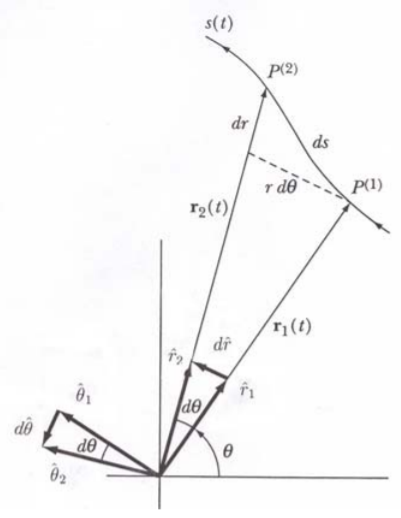
The complication and implications of time-dependent unit vectors are best illustrated by considering twodimensional polar coordinates which is the simplest curvilinear coordinate system. Polar coordinates are a special case of cylindrical coordinates, when z is held fixed, or a special case of spherical coordinate system, when ϕ is held fixed.
Consider the motion of a point P as it moves along a curve s(t) such that in the time interval dt it moves from P(1) to P(2) as shown in Figure 19.4.1. The two-dimensional polar coordinates have unit vectorsr^,θ^, which are orthogonal and change from r^1,θ^1, to r^2,θ^2, in the time dt. Note that for these polar coordinates the angle unit vector θ^ is taken to be tangential to the rotation since this is the direction of motion of a point on the circumference at radius r.
The net changes shown in figure of Table 19.4.2 are
dr^=r^2−r^1=dr^=∣r^∣dθθ^=dθθ^(C.9)
since the unit vector r^ is a constant with ∣r^∣=1. Note that the infinitesimal dr^ is perpendicular to the unit vector r^, that is, dr^ points in the tangential direction θ^.
Similarly, the infinitesimal
dθ^=θ^2−θ^1=dθ^=−dθr^(C.10)
which is perpendicular to the tangential θ^ unit vector and therefore points in the direction −r^. The minus sign causes −dθr^ to be directed in the opposite direction to r^.
The net distance element ds is given by
ds=drr^+rdr^=drr^+rdθθ^(C.11)
This agrees with the prediction obtained using Table 19.4.1.
The time derivatives of the unit vectors are given by equations C.9 and C.10 to be,
dtdr^=dtdθθ^(C.12)
dtdθ^=−dtdθr^(C.13)
Note that the time derivatives of unit vectors are perpendicular to the corresponding unit vector, and the unit vectors are coupled.
where the rθ˙2r^ term is the effective centripetal acceleration while the 2r˙θ˙θ^ term is called the Coriolis term. For the case when r˙=r¨=0, then the first bracket in C.15 is the centripetal acceleration while the second bracket is the tangential acceleration.
This discussion has shown that in contrast to the time independence of the cartesian unit basis vectors, the unit basis vectors for curvilinear coordinates are time dependent which leads to components of the velocity and acceleration involving coupled coordinates.
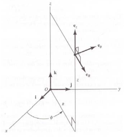
The three-dimensional cylindrical coordinates (ρ,ϕ,z) are obtained by adding the motion along the symmetry axis z^ to the case for polar coordinates. The unit basis vectors are shown in Table 19.4.3 where the angular unit vector ϕ^ is taken to be tangential corresponding to the direction a point on the circumference would move. The distance and volume elements, the cartesian coordinate components of the cylindrical unit basis vectors, and the unit vector time derivatives are shown in Table 19.4.3. The time dependence of the unit vectors is used to derive the acceleration. As for the two-dimensional polar coordinates, the ρ^ and θ^ direction components of the acceleration for cylindrical coordinates are coupled functions of ρ, ρ˙, ρ¨, ϕ˙, and ϕ¨.
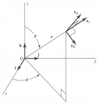
The three dimensional spherical coordinates, can be treated the same way as for cylindrical coordinates. The unit basis vectors are shown in Table 19.4.4 where the angular unit vectors θ^ and ϕ^ are taken to be tangential corresponding to the direction a point on the circumference moves for a positive rotation angle.
The distance and volume elements, the cartesian coordinate components of the spherical unit basis vectors, and the unit vector time derivatives are shown in the table given in Figure 19.4.3. The time dependence of the unit vectors is used to derive the acceleration. As for the case of cylindrical coordinates, the r^, θ^, and ϕ^ components of the acceleration involve coupling of the coordinates and their time derivatives.
It is important to note that the angular unit vectors θ^ and ϕ^ are taken to be tangential to the circles of rotation. However, for discussion of angular velocity of angular momentum it is more convenient to use the axes of rotation defined by r^×θ^ and r^×ϕ^ for specifying the vector properties which is perpendicular to the unit vectors θ^ and ϕ^. Be careful not to confuse the unit vectors θ^ and ϕ^ with those used for the angular velocities θ˙ and ϕ˙.
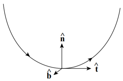
The cartesian, polar, cylindrical, or spherical curvilinear coordinate systems, all are orthogonal coordinate systems that are fixed in space. There are situations where it is more convenient to use the Frenet-Serret coordinates which comprise an orthogonal coordinate system that is fixed to the particle that is moving along a continuous, differentiable, trajectory in three-dimensional Euclidean space. Let s(t) represent a monotonically increasing arc-length along the trajectory of the particle motion as a function of time t. The Frenet-Serret coordinates, shown in Figure 19.4.4, are the three instantaneous orthogonal unit vectors t^, n^, and b^ where the tangent unit vector t^ is the instantaneous tangent to the curve, the normal unit vector n^ is in the plane of curvature of the trajectory pointing towards the center of the instantaneous radius of curvature and is perpendicular to the tangent unit vector t^, while the binormal unit vector is b^=t^×n^ which is the perpendicular to the plane of curvature and is mutually perpendicular to the other two Frenet-Serrat unit vectors. The Frenet-Serret unit vectors are defined by the relations
dsdt^=κn^(C.16)
dsdb^=−τn^(C.17)
dsdn^=−κt^+τb^(C.18)
The curvature κ=ρ1 where ρ is the radius of curvature and τ is the torsion that can be either positive or negative. For increasing s, a non-zero curvature κ implies that the triad of unit vectors rotate in a right-handed sense about b^. If the torsion τ is positive (negative) the triad of unit vectors rotates in right (left) handed sense about t^.
In general the Frenet-Serret unit vectors are time dependent. If the curvature κ=0 then the curve is a straight line and n^ and b^ are not well defined. If the torsion is zero then the trajectory lies in a plane. Note that a helix has constant curvature and constant torsion.
The rate of change of a general vector field E along the trajectory can be written as
dsdE=(dsdEtt^+dsdEnn^+dsdEbb^)+ω×E(C.23)
The Frenet-Serret coordinates are used in the life sciences to describe the motion of a moving organism in a viscous medium. The Frenet-Serret coordinates also have applications to General Relativity.
The goal of this problem is to help you understand the origin of the equations that relate two different coordinate systems. Refer to diagrams for cylindrical and spherical coordinates as your teaching assistant explains how to arrive at expressions for x1, x2, and x3 in terms of ρ, ϕ, and z and how to derive expressions for the velocity and acceleration vectors in cylindrical coordinates. Now try to relate spherical and rectangular coordinate systems. Your group should derive expressions relating the coordinates of the two systems, expressions relating the unit vectors and their time derivatives of the two systems, and finally, expressions for the velocity and acceleration in spherical coordinates.
Coordinate systems can be translated, or rotated with respect to each other as well as being subject to spatial inversion or time reversal. Scalars, vectors, and tensors are defined by their transformation properties under rotation, spatial inversion and time reversal, and thus such transformations play a pivotal role in physics.
Translational transformations are involved frequently for transforming between the center of mass and laboratory frames for reaction kinematics as well as when performing vector addition of central forces for the cases where the centers are displaced. Both the classical Galilean transformation or the relativistic Lorentz transformation are handled the same way. Consider two parallel orthonormal coordinate frames where the origin of F′(x′,y′,z′) is displaced by a time dependent vector a(t) from the origin of frame F(x,y,z). Then the Galilean transformation for a vector r in frame F to r′ in frame F′ is given by
r(x′,y′,z′)=r(x,y,z)+a(t)(D.1)
The velocities for a moving frame are given by the vector difference of the velocity in a stationary frame, and the velocity of the origin of the moving frame. Linear accelerations can be handled similarly.
Rotational transformations of the coordinate system are used extensively in physics. The transformation properties of fields under rotation define the scalar and vector properties of fields, as well as rotational symmetry and conservation of angular momentum.
Rotation of the coordinate frame does not change the value of any scalar observable such as mass, temperature etc. That is, transformation of a scalar quantity is invariant under coordinate rotation from x,y,z→x′,y′,z′.
ϕ(x′y′z′)=ϕ(xyz)(D.2)
By contrast, the components of a vector along the coordinate axes change under rotation of the coordinate axes. This difference in transformation properties under rotation between a scalar and a vector is important and defines both scalars and a vectors.
Matrix mechanics, described in appendix 19.1, provides the most convenient way to handle coordinate rotations. The transformation matrix, between coordinate systems having differing orientations is called the rotation matrix. This transforms the components of any vector with respect to one coordinate frame to the components with respect to a second coordinate frame rotated with respect to the first frame.
Assume a point P has coordinates (x1,x2,x3) with respect to a certain coordinate system. Consider rotation to another coordinate frame for which the point P has coordinates (x1′,x2′,x3′) and assume that the origins of both frames coincide. Rotation of a frame does not change the vector, only the vector components of the unit basis states. Therefore
Note that if one designates that the unit vectors for the unprimed coordinate frame are (e^1,e^2,e^3) and for the primed coordinate frame (e^1′,e^2′,e^3′), then taking the scalar product of Equation D.3 sequentially with each of the unit base vectors (e^1′,e^2′,e^3′) leads to the following three relations
Note that the (e^i′⋅e^j) are the direction cosines as defined by the scalar product of two unit vectors for axes i,j, that is, they are the cosine of the angle between the two unit vectors.
The inverse procedure is obtained by multiplying Equation D.3 successively by one of the unit basis vectors (e^1,e^2,e^3) leading to three equations
Consider an arbitrary rotation through an angle θ. Equations D.10 and D.11 can be used to relate six of the nine quantities λij in the rotation matrix, so only three of the quantities are independent. That is, because of Equation D.11 we have three equations which ensure that the transformation is unitary.
λi12+λi22+λi32=1(D.12)
Also requiring that the axes be orthogonal gives three equations
j∑λijλkj=0,i=k(D.13)
These six relations can be expressed as
j∑λijλkj=δik(D.14)
The fact that the rotation matrix should have three independent quantities is due to the fact that all rotations can be expressed in terms of rotations about three orthogonal axes.
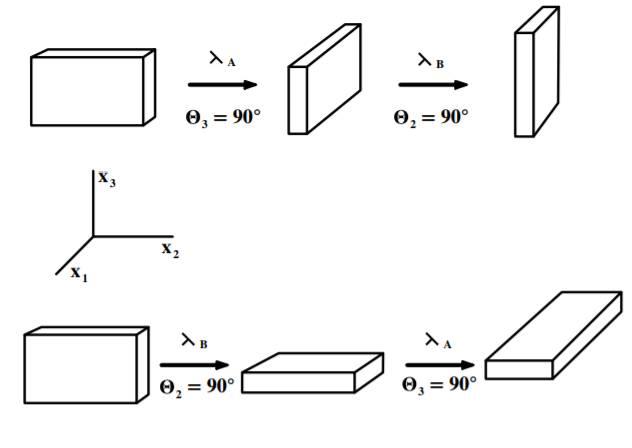
Figure 19.5.2:Order of two finite rotations for a parallelepiped.
Consider two finite 90∘ rotations λA and λB illustrated in Figure 19.5.2. The λA rotation is 90∘ around the x3 axis in a right-handed direction as shown. In such a rotation the axes transform to x1′=x2,x2′=−x1,x3′=x3 and the rotation matrix is
λA=⎝⎛0−10100001⎠⎞(D.15)
The second rotation λB is a right-handed rotation about the x1′ axis which formerly was the x2 axis. Then x1"=x2′,x2"=−x1′,x3"=x3′ and the rotation matrix is
λB=⎝⎛10000−1010⎠⎞(D.16)
Consider the product of these two finite rotations which corresponds to a single rotation matrix λAB
An entirely different orientation results as illustrated in Figure 19.5.2.
This behavior of finite rotations is a consequence of the fact that finite rotations do not commute, that is, reversing the order does not give the same answer. Thus, if we associate the vectors A and B with these rotations, then it implies that the vector product AB=BA. That is, for finite rotation matrices, the product does not behave like for true vectors since they do not commute.
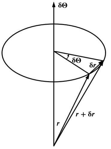
Infinitesimal rotations do not suffer from the noncommutation defect of finite rotations. If the position vector of a point changes from r to r+δr then the geometrical situation is represented correctly by
δr=δθ×r(D.21)
where δθ is a quantity whose magnitude is equal to the infinitesimal rotation angle and which has a direction along the instantaneous axis of rotation as illustrated in Figure 19.5.3.
The infinitesimal angle δθ is a vector which is shown by proving that two infinitesimal rotations δθ1 and δθ2 commute. The change in position vectors of the point are
δr1=δθ1×r(D.22)
and
δr2=δθ2×(r+δr1)(D.23)
Thus the final position vector for δθ1 followed by δθ2 is
r+δr1+δr2=r+δθ1×r+δθ2×(r+δr1)(D.24)
Assuming that the second-order infinitesimals can be ignored gives
r+δr1+δr2=r+δθ1×r+δθ2×r(D.25)
Consider now the inverse order of rotations.
r+δr2+δr1=r+δθ2×r+δθ1×(r+δr2)(D.26)
Again, neglecting the second-order infinitesimals gives
r+δr2+δr1=r+δθ2×r+δθ1×r(D.27)
Note that the products of these two infinitesimal rotations, D.25 and D.27 are identical. That is, assuming that second-order infinitesimals can be neglected, then the infinitesimal rotations commute, and thus δθ1 and δθ2 are correctly represented by vectors.
The fact that δθ is a vector allows angular velocity to be represented by a vector. That is, angular velocity is the ratio of an infinitesimal rotation to an infinitesimal time.
ω=δtδθ(D.28)
Note that this implies that the velocity of the point can be expressed as
The requirement that the coordinate axes be orthogonal, and that the transformation be unitary, leads to the relation between the components of the rotation matrix.
j∑λijλkj=δik(D.30)
It was shown in equation (19.1.12) that, for such an orthogonal matrix, the inverse matrix λ−1 equals the transposed matrix λT
λ−1=λT
Inserting the orthogonality relation for the rotation matrix leads to the fact that the square of the determinant of the rotation matrix equals one,
∣λ∣2=1(D.31)
that is
∣λ∣=±1(D.32)
A proper rotation is the rotation of a normal vector and has
∣λ∣=+1(D.33)
An improper rotation corresponds to
∣λ∣=−1(D.34)
An improper rotation implies a rotation plus a spatial reflection which cannot be achieved by any combination of only rotations.
Consider the cross product of two vectors c=a×b. It can be shown that the cross product behaves under rotation as:
ci′=∣λ∣j∑λijcj(D.35)
For all proper rotations the determinant of λ=+1 and thus the cross product also acts like a proper vector under rotation. This is not true for improper rotations where ∣λ∣=−1.
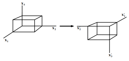
Spatial inversion, that is, mirror reflection, corresponds to reflection of all coordinate vectors, i=−i, j=−j, and k=−k. Such a transformation corresponds to the transformation matrix
λ=⎝⎛−1000−1000−1⎠⎞=−⎝⎛100010001⎠⎞(D.36)
Figure 19.5.4:Inversion of an object corresponds to reflection about the origin of all axes.
Thus ∣λ∣=−1, that is, it corresponds to an improper rotation. A spatial inversion for two vectors A(r) and B(r) correspond to
A(r)=−A(−r)B(r)=−B(−r)(D.37)
That is, normal polar vectors change sign under spatial reflection. However, the cross product C=A×B does not change sign under spatial inversion since the product of the two minus signs is positive. That is,
C(r)=+C(−r)(D.38)
Thus the cross product behaves differently from a polar vector. This improper behavior is characteristic of an axial vector, which also is called a pseudovector.
Examples of pseudovectors are angular momentum, spin, magnetic field etc. These pseudovectors are defined using the right-hand rule and thus have handedness. For a right-handed system
CR=A×B(D.39)
Changing to a left-handed system leads to
CL=B×A=−A×B(D.40)
That is, handedness corresponds to a definite ordering of the cross product. Proper orthogonal transformations are said to preserve chirality (Greek for handedness) of a coordinate system.
An example of the use of the right-handed system is the usual definition of cartesian unit vectors,
i×j=k(D.41)
An obvious question to be asked, is the handedness of a coordinate system merely a mathematical curiosity or does it have some deep underlying significance? Consider the Lorentz force
F=q(E+v×B)(D.42)
Since force and velocity are proper vectors then the magnetic B field must be a pseudo vector. Note that calculation of the B field occurs only in cross products such as,
∇×B=μj(D.43)
where the current density j is a proper vector. Another example is the Biot-Savart Law which expresses B as
dB=4πμoIr2dl×r(D.44)
Thus even though B is a pseudo vector, the force F remains a proper vector. Thus if a left-handed coordinate definition of BL=4πμoIr2r×dl is used in D.44, and F=q(E+BL×v) in D.42, then the same final physical result would be obtained.
It was long thought that the laws of physics were symmetric with respect to spatial inversion ( i.e. mirror reflection), meaning that the choice between a left-handed and right-handed representations (chirality) was arbitrary. This is true for gravitational, electromagnetic and the strong force, and is called the conservation of parity. The fourth fundamental force in nature, the weak force, violates parity and favors handedness. It turns out that right-handed ordinary matter is symmetrical with left-handed antimatter.
In addition to the two flavors of vectors, one has scalars and pseudoscalars defined by:
ϕ(r)=+ϕ(−r)(D.45)
ϕ(r)=−ϕ(−r)(D.46)
An example of a pseudoscalar is the scalar product A⋅(B×C)
The basic laws of classical mechanics are invariant to the sense of the direction of time. Under time reversal the vector r is unchanged while both momentum p and time t change sign under time reversal, thus the time derivative F=dtdp is invariant to time reversal; that is, the force is unchanged and Newton’s Laws F=dtdp are invariant under time reversal. Since the force can be expressed as the gradient of a scalar potential for a conservative field, then the potential also remains unchanged. That is
dtdp=−∇U(r)=F(D.47)
It is necessary to introduce tensor algebra, given in appendix 19.5, prior to discussion of the transformation properties of observables which is the topic of appendix 19.5.5.
Suppose the x2-axis of a rectangular coordinate system is rotated by 30∘ away from the x3-axis around the x1-axis.
(a) Find the corresponding transformation matrix. Try to do this by drawing a diagram instead of going to the book or the notes for a formula.
(b) Is this an orthogonal matrix? If so, show that it satisfies the main properties of an orthogonal matrix. If not, explain why it fails to be orthogonal.
(c) Does this matrix represent a proper or an improper rotation? How do you know?
When you were first introduced to vectors, you most likely were told that a scalar is a quantity that is defined by a magnitude, while a vector has both a magnitude and a direction. While this is certainly true, there is another, more sophisticated way to define a scalar quantity and a vector quantity: through their transformation properties. A scalar quantity transforms as ϕ′=ϕ while a vector quantity transforms as Ai′=∑jλijAj. To show that the scalar product does indeed transform as a scalar, note that:
Now you will show that the vector product transforms as a vector. Begin by writing out what you are trying to show explicitly and show it to the teaching assistant. Once the teaching assistant has confirmed that you have the correct expression, try to prove it. The vector product is a bit more difficult to work with than the scalar product, so your teaching assistant is prepared to give you a hint if you get stuck.
Suppose you have two rectangular coordinate systems that share a common origin, but one system is rotated by an angle θ with respect to the other. To describe this rotation, you have made use of the rotation matrix λ(θ). (I’m changing the notation slightly to put the emphasis on the angle of rotation.)
(a) Verify that the product of two rotation matrices λ(θ1)λ(θ2) is in itself a rotation matrix.
(b) In abstract algebra, a group G is defined as a set of elements g together with a binary operation ∗ acting on that set such that four properties are satisfied:
i. (Closure) For any two elements gi and gj in the group G, the product of the elements, gi∗gj is also in the group G.
ii. (Associativity) For any three elements gi,gj,gk of the group G, (gi∗gj)∗gk=gi∗(gj∗gk).
iii. (Existence of Identity) The group G contains an identity element e such that g∗e=e∗g=g for all g∈G.
iv. (Existence of Inverses) For each element g∈G, there exists an inverse element g−1∈G such that g∗g−1=g−1∗g=e.
Show that if the product ∗ denotes the product of two matrices, then the set of rotation matrices together with ∗ forms a group. This group is known as the special orthogonal group in two dimensions, also known as SO(2).
(c) Is this group commutative? In abstract algebra, a commutative group is called an abelian group.
When you look in a mirror the image of you appears left-to-right reversed, that is, the image of your left ear appears to be the right ear of the image and vice versa. Explain why the image is left-right reversed rather than up-down reversed or reversed about some other axis; i.e. explain what breaks the symmetry that leads to these properties of the mirror image.
Find the transformation matrix that rotates the axis x3 of a rectangular coordinate system 45∘ toward x1 around the x2 axis.
For simplicity, take λ to be a two-dimensional transformation matrix. Show by direct expansion that ∣λ∣2=1.
Mathematically scalars and vectors are the first two members of a hierarchy of entities, called tensors, that behave under coordinate transformations as described in appendix 19.4. The use of the tensor notation provides a compact and elegant way to handle transformations in physics.
A scalar is a rank 0 tensor with one component, that is invariant under change of the coordinate system.
ϕ(x′y′z′)=ϕ(xyz)(E.1)
A vector is a rank 1 tensor which has three components, that transform under rotation according to matrix relation
x′=λ⋅x(E.2)
where λ is the rotation matrix. Equation E.2 can be written in the suffix form as
xi′=j=1∑3λijxj(E.3)
The above definitions of scalars and vectors can be subsumed into a class of entities called tensors of rank n that have 3n components. A scalar is a tensor of rank r=0, with only 30=1 component, whereas a vector has rank r=1, that is, the vector x has one suffix i and 31=3 components.
A second-order tensor Tij has rank r=2 with two suffixes, that is, it has 32=9 components that transform under rotation as
Tij′=k=1∑3l=1∑3λikλjlTkl(E.4)
For second-order tensors, the transformation formula given by Equation E.4 can be written more compactly using matrices. Thus the second-order tensor can be written as a 3×3 matrix
where λljT are the matrix elements of the transposed matrix λT. The summations in E.6 can be expressed in both the tensor and conventional matrix form as the matrix product
T′=λ⋅T⋅λT(E.7)
Equation E.7 defines the rotational properties of a spherical tensor.
Tensor products feature prominently when using tensors to represent transformations. A second-order tensor T can be formed by using the tensor product, also called outer product, of two vectors a and b which, written in suffix form, is
In component form the matrix elements of this matrix are given by
Tij=aibj(E.9)
This second-order tensor product has a rank r=2, that is, it equals the sum of the ranks of the two vectors. Equation E.8 is called a dyad since it was derived by taking the dyadic product of two vectors. In general, multiplication, or division, of two vectors leads to second-order tensors. Note that this second-order tensor product completes the triad of tensors possible taking the product of two vectors. That is, the scalar product a⋅b, has rank r=0, the vector product a×b, rank r=1 and the tensor product a⊗b has rank[1]r=2.
Higher-order tensors can be created by taking more complicated tensor products. For example, a rank-3 tensor can be created by taking the tensor outer product of the rank-2 tensor Tij and a vector ck which, for a dyadic tensor, can be written as the tensor product of three vectors. That is,
Tijk=Tijck=aibjck(E.10)
In summary, the rank of the tensor product equals the sum of the ranks of the tensors included in the tensor product.
The lowest rank tensor product, which is called the inner product, is obtained by taking the tensor product of two tensors for the special case where one index is repeated, and taking the sum over this repeated index. Summing over this repeated index, which is called contraction, removes the two indices for which the index is repeated, resulting in a tensor that has rank r equal to the sum of the ranks minus 2 for one contraction. That is, the product tensor has rank r=r1+r2−2.
The simplest example is the inner product of two vectors which has rank r=1+1−2=0, that is, it is the scalar product that equals the trace of the inner product matrix, and this inner product is commutative.
An especially important case is the inner product of a rank-2 dyad a⊗b, given by Equation E.8, with a vector c, that is, the inner product T=a⊗b⋅c. Written in component form, the inner product is
i∑3aibicj=(i∑3aibi)cj=(a⋅b)cj(E.11)
The scalar product a⋅b is a scalar number, and thus the inner-product tensor is the vector c renormalized by the magnitude of the scalar product a⋅b. That is, it has a rank r=2+1−2=1. Thus the inner product of this rank-2 tensor with a vector gives a vector. The inner product of a rank-2 tensor with a rank-1 tensor is used in this book for handling the rotation matrix, the inertia tensor for rigid-body rotation, and for the stress and the strain tensors used to describe elasticity in solids.
In principle one must distinguish between a 3×3 square matrix, and the tensor component representations of a rank-2 tensor. However, as illustrated by the previous discussion, for orthogonal transformations, the tensor components of the second rank tensor transform identically with the matrix components. Thus functionally, the matrix formulation and tensor representations are identical. As a consequence, all the terminology and operations used in matrix mechanics are equally applicable to the tensor representation.
The tensor representation of the rotation matrix provides the simplest example of the equivalence of the matrix and tensor representations of transformations. Appendix 19.4.2 showed that the unitary rotation matrix λ, acting on a vector x transforms it to the vector x′ that is rotated with respect to x. That is, the transformation is
Appendix 19.4.2 showed that the rotation matrix λ requires 9 components to fully specify the transformation from the initial 3-component vector x to the rotated vector x′. The rotation tensor is a dyad as well as being unitary and dimensionless. Note that Equation D5 is an example of the inner product of a rank−2 rotation tensor acting on a vector leading to a another vector that is rotated with respect to the first vector.
In general, rank-2 tensors have dimensions and are not unitary. For example, the angular velocity vector ω and the angular momentum vector L are related by the inner product of the inertia tensor {I} and ω. That is
L={I}⋅ω(11.6)
The inertia tensor has dimensions of mass×length2 and relates two very different vector observables. The stress tensor and the strain tensor, discussed in chapter 15, provide another example of second-order tensors that are used to transform one vector observable to another vector observable analogous to the case of the rotation matrix or the inertia tensor.
Note that pseudo-tensors can be used to make a rotational transformation plus a change in the sign. That is, they lead to a parity inversion.
The tensor notation is used extensively in physics since it provides a powerful, elegant, and compact representation for describing transformations.
In general the configuration space used to specify a dynamical system is not a Euclidean space in that there may not be a system of coordinates for which the distance between any two neighboring points can be represented by the sum of the squares of the coordinate differentials. For example, a set of cartesian coordinate does not exist for the two-dimension motion of a single particle constrained to the curved surface of a fixed sphere. Such curved spaces need to be represented in terms of Riemannian geometry rather than Euclidean geometry. Curved configuration spaces occur in some branches of physics such as Einstein’s General Theory of Relativity.
Tensors have transformation properties that can be either contravariant or covariant. Consider a set of generalized coordinates q′ that are a function of the coordinates q. Then infinitesimal changes dqm will lead to infinitesimal changes dq′n where
dq′n=m∑∂qm∂q′ndqm(E.12)
Contravariant components of a tensor transform according to the relation
λ′n=m∑∂qm∂q′nλm(E.13)
Equation E.13 relates the contravariant components in the unprimed and primed frames.
Derivatives of a scalar function ϕ, such as
λn′=∂qn∂ϕ=m∑∂qm∂ϕ∂qn∂qm=m∑∂qn∂qmλm(E.14)
That is, covariant components of the tensor transform according to the relation
λn′=m∑∂qn∂qmλm(E.15)
It is important to differentiate between contravariant and covariant vectors. The superscript/subscript convention for distinguishing between these two flavors of tensors is given in table 19.6.1
xμ
denotes a contravariant vector
xν
denotes a covariant vector
In linear algebra one can map from one coordinate system to another as illustrated in appendix 19.4. That is, the tensor x can be expressed as components with respect to either the unprimed or primed coordinate frames
For a n−dimensional manifold the unit basis column vectors e^ transform according to the transformation matrix λ
e^′=λ⋅e^(E.17)
Since the tensor x is independent of the coordinate basis, the components of x must have the opposite transform
x′=(λ−1)T⋅x(E.18)
This normal vector x is called a “contravariant vector” because it transforms contrary to the basis column vector transformation.
The inverse of Equation E.18 gives that the column vector element
xμ=ν∑λμνxν′(E.19)
Consider the case of a gradient with respect to the coordinate x in both the unprimed and primed bases. Using the chain rule for the partial derivative then the component of the gradient in the primed frame can be expanded as
That is, a gradient transforms as a covariant vector, like the unit vectors, whereas a vectorxis contravariant under transformation.
Normally the basis is orthonormal, (λ−1)T=λ, and thus there is no difference between contravariant and covariant vectors. However, for curved coordinate systems, such as non-Euclidean geometry in the General Theory of Relativity, the covariant and contravariant vectors behave differently.
The Einstein convention is extended to apply to matrices by writing the elements of the matrix A as Aνμ while the elements of the transposed matrix A−1 are written as Aμν. The matrix product for A with a contravariant vector X is written as
X′μ=ν∑AνμXν(E.22)
where the summation over ν effectively cancels the identical superscript and subscript ν.
Similarly a covariant vector, such as a gradient, is written as,
where gμν is a unitary matrix called a covariant metric. The covariant metric transforms a contravariant to a covariant tensor. For example the matrix element of a covariant tensor Xν can be written as
Xν=μ∑gμνXμ(E.26)
By association of the covariant metric with either of the vectors in the inner product gives
S=μν∑gμνXμYν=ν∑XνYν=μ∑XμYμ(E.27)
Similarly it can be defined in terms of an orthogonal contravariant metricgμν where
S=μν∑gμνXμYν(E.28)
Then
Xν=μ∑gμνXμ(E.29)
Association of the contravariant metric with one of the vectors in the inner product gives the inner product
S=μν∑gμνXμYν=ν∑XνYν=μ∑XμYμ(E.30)
For most situations in this book the metric gμν is diagonal and unitary.
In physics, observables can be represented by spherical tensors which specify the angular momentum and parity characteristics of the observable, and the tensor rank is independent of the time dependence. The transformation properties of these tensors, coupled with their time-reversal invariance, specify the fundamental characteristics of the observables.
Table 19.6.2 summarizes the transformation properties under rotation, spatial inversion and time reversal for observables encountered in classical mechanics and electrodynamics. Note that observables can be scalar, vector, pseudovector, or second-order tensors, under rotation, and even or odd under either space inversion or time inversion. For example, in classical mechanics the inertia tensor I relates the angular velocity vector ω to the angular momentum vector L by taking the inner product L=I⋅ω. In general I is not diagonal and thus the angular momentum is not parallel to the angular velocity ω. A similar example in electrodynamics is the dielectric tensor K which relates the displacement field D to the electric field E by D=K⋅E. For anisotropic crystal media K is not diagonal leading to the electric field vectors E and D not being parallel.
As discussed in chapter 7, Noether’s Theorem states that symmetries of the transformation properties lead to important conservation laws. The behavior of classical systems under rotation relates to the conservation of angular momentum, the behavior under spatial inversion relates to parity conservation, and time-reversal invariance relates to conservation of energy. That is, conservative forces conserve energy and are time-reversal invariant.
Physical Observable
Rotation (Tensor rank)
Space inversion
Time reversal
Name
1) Classical Mechanics
Mass density
ρ
0
Even
Even
Scalar
Kinetic energy
p2/2m
0
Even
Even
Scalar
Potential energy
U(r)
0
Even
Even
Scalar
Lagrangian
L
0
Even
Even
Scalar
Hamiltonian
H
0
Even
Even
Scalar
Gravitational potential
ϕ
0
Even
Even
Scalar
Coordinate
r
1
Odd
Even
Vector
Velocity
v
1
Odd
Odd
Vector
Momentum
p
1
Odd
Odd
Vector
Angular momentum
L=r×p
1
Even
Odd
Pseudovector
Force
F
1
Odd
Even
Vector
Torque
N=r×F
1
Even
Even
Pseudovector
Gravitational field
g
1
Odd
Even
Vector
Inertia tensor
I
2
Even
Even
Tensor
Elasticity stress tensor
Tik
2
Even
Even
Tensor
2) Electromagnetism
Charge density
ρ
0
Even
Even
Scalar
Current density
j
1
Odd
Odd
Vector
Electric field
E
1
Odd
Even
Vector
Polarization
P
1
Odd
Even
Vector
Displacement
D
1
Odd
Even
Vector
Magnetic B field
B
1
Even
Odd
Pseudovector
Magnetization
M
1
Even
Odd
Pseudovector
Magnetic H field
H
1
Even
Odd
Pseudovector
Poynting vector
S=E×H
1
Odd
Odd
Vector
Dielectric tensor
K
2
Even
Even
Tensor
Maxwell stress tensor
Tik
2
Even
Even
Tensor
2Based on table 6.1 in “Classical Electrodynamics”2nd edition, by J.D. Jackson [Jac75]
19.7: Appendix - Aspects of Multivariate Calculus¶
Multivariate calculus provides the framework for handling systems having many variables associated with each of several bodies. It is assumed that the reader has studied linear differential equations plus multivariate calculus and thus has been exposed to the calculus used in classical mechanics. Chapter 5 of this book introduced variational calculus which covers several important aspects of multivariate calculus such as Euler’s variational calculus and Lagrange multipliers. This appendix provides a brief review of a selection of other aspects of multivariate calculus that feature prominently in classical mechanics.
The extension of the derivative to multivariate calculus involves use of partial derivatives. The partial derivative with respect to the variable xi of a multivariate function f(x1,x2,....,xN) involves taking the normal one-variable derivative with respect to xi assuming that the other N−1 variables are held constant. That is,
where it will be assumed that the function f(x) is a continuously-differentiable function to nth order, then all partial derivatives of that order or less are independent of the order in which they are performed. That is,
∂xi∂xj∂2f(x)=∂xj∂xi∂2f(x)(F.2)
The chain rule for partial differentiation gives that
The linear operator notation provides a powerful, elegant, and compact way to express, and apply, the equations of multivariate calculus; it is used extensively in mathematics and physics. The linear operators typically comprise partial derivatives that act on scalar, vector, or tensor fields. Table 19.7.1 lists a few elementary examples of the use of linear operators in this textbook. The first four linear operators involve the widely used del operator ∇ to generate the gradient, divergence and curl as described in appendices 19.7 and 19.8. The fifth and sixth linear operators act on the Lagrangian in Lagrangian mechanics applications. The final two linear operators act on the wavefunction for wave mechanics.
Name
Partial derivative
Field
Action
Gradient
∇≡i^∂x∂+j^∂y∂+k^∂z∂
Scalar potential V
E=∇V
Divergence
∇⋅≡(i^∂x∂+j^∂y∂+k^∂z∂)⋅
Vector field E
∇⋅E
Curl
∇×≡(i^∂x∂+j^∂y∂+k^∂z∂)×
Vector field E
∇×E
Laplacian
∇2=∇⋅∇≡∂x2∂2+∂y2∂2+∂z2∂2
Scalar potential V
∇2V
Euler-Lagrange
Λj≡dtd∂q˙j∂−∂qj∂
Scalar Lagrangian L
ΛL=0
Canonical momentum
pj≡∂q˙j∂
Scalar Lagrangian L
pj≡∂q˙j∂L
Canonical momentum
pj≡iℏ∂q˙j∂
Wavefunction Ψ
pjΨ≡iℏ∂q˙j∂Ψ
Hamiltonian
H=iℏ∂t∂
Wavefunction Ψ
HΨ=iℏ∂t∂Ψ=EΨ
There are three ways of expressing operations such as addition, multiplication, transposition or inversion of operations that are completely equivalent because they all are based on the same principles of linear algebra. For example, a transformation O acting on a vector A can produce the vector B. The simplest way to express this transformation is in terms of components
Bi=j=1∑3OijAj(F.6)
Another way is to use matrix mechanics where the 3×3 matrix (O) transforms the column vector (A) to the column vector (B), that is,
(B)=(O)(A)(F.7)
The third approach is to assume an operator O acts on the vector A
B=OA(F.8)
In classical mechanics, and quantum mechanics, these three equivalent approaches are used and exploited extensively and interchangeably. In particular the rules of matrix manipulation, that are given in appendix 19.1, are synonymous, and equivalent to, those that apply for operator manipulation. If the operator is complex then the operator properties are summarized as follows.
The generalization of the transpose for complex operators is the Hermitian conjugateO†
Oij†=Oji∗(F.9)
Note also that
O†=(O∗)T=(OT)∗(F.10)
The generalization of a symmetric matrix is Hermitian, that is, O is equal to its Hermitian conjugate
Oij†=Oji∗=Oij(F.11)
For a real matrix the complex conjugation has no effect so the matrix is real and symmetric.
The generalization of orthogonal is unitary for which the operator is unitary if it is non-singular and
The Jacobian determinant, which is usually called the Jacobian, is used extensively in mechanics for both rotational and translational coordinate transformations. The Jacobian determinant is defined as being the ratio of the n-dimensional volume element dx1dx2...dxn in one coordinate system, to the volume element dy1dy2...dyn in the second coordinate system. That is
Consider a coordinate transformation for the integral of the function f(x1,x2,..xn) to the integral of a function g(y1,y2,...yn) where yi=h(x1,x2,...xn). The coordinate transformation of the integral equation can be expressed in terms of the Jacobian J(y1y2...yn)
The differential cross sections for scattering can be defined either by the number of a definite kind of particle/per event, going into the volume element in momentum space dp1dp2dp3, or by the number going into the solid angle element having momentum between p and p+dp. That is, the first definition can be written as a differential equation
In classical mechanics the Jacobian often is extended from 3 dimensions to n-dimensional transformations. The Jacobian is unity for unitary transformations such as rotations and linear translations which implies that the volume element is preserved. It will be shown that this also is true for a certain class of transformations in classical mechanics that are called canonical transformations. The Jacobian transforms the local density to be correct for any scale transformations such as transforming linear dimensions from centimeters to inches.
Hamiltonian mechanics can be derived directly from Lagrange mechanics by considering the Legendre transformation between the conjugate variables (q,q˙,t) and (q,p,t). Such a derivation is of considerable importance in that it shows that Hamiltonian mechanics is based on the same variational principles as those used to derive Lagrangian mechanics; that is d’Alembert’s Principle or Hamilton’s Principle. The general problem of converting Lagrange’s equations into the Hamiltonian form hinges on the inversion of equation (8.1.3) that defines the generalized momentum p. This inversion is simplified by the fact that (8.1.3) is the first partial derivative of the Lagrangian L(q,q˙,t) which is a scalar function.
Consider transformations between two functions F(u,w) and G(v,w) where u and v are the active variables related by the functional form
v=∇uF(u,w)(F.19)
and where w designates passive variables and ∇uF(u,w) is the first-order derivative of F(u,w), i.e. the gradient, with respect to the components of the vector u. The Legendre transform states that the inverse formula can always be written in the form
u=∇vG(v,w)(F.20)
where the function G(v,w) is related to F(u,w) by the symmetric relation
G(v,w)+F(u,w)=u⋅v(F.21)
and where the scalar product u⋅v=∑i=1Nuivi.
Furthermore the derivatives with respect to all the passive variables {wi} are related by
∇wF(u,w)=−∇wG(v,w)(F.22)
The relationship between the functions F(u,w) and G(v,w) is symmetrical and each is said to be the Legendre transform of the other.
Below you will find a set of integrals. Your teaching assistant will divide you into groups and each group will be assigned one integral to work on. Once your group has solved the integral, write the solution on the board in the space provided by the teaching assistant.
(a) ∫02π∫0π/4∫0cosθr2sinθdrdθdϕ
(b) ∫(rr˙−r2rr˙)dt
(c) ∫SA⋅da where A=xi^+yj^+zk^ and S is the sphere x2+y2+z2=9.
(d) ∫S(∇×A)⋅da where A=yi^+zj^+xk^ and S is the surface defined by the paraboloid z=1−x2−y2, where z≥0.
Differential operators like time (dtd) do not change the rotational properties of scalars or proper vectors. A scalar operator dsd acting on a scalar field ϕ(xyz), in a rotated coordinated frame ϕ′(x′y′z′) is unchanged.
That is, differentiation of scalar or vector fields with respect to a scalar operator does not change the rotational behavior. In particular, the scalar differentials of vectors continue to obey the rules of ordinary proper vectors. The scalar operator ∂t∂ is used for calculation of velocity or acceleration.
Vector differential operators in cartesian coordinates¶
Vector differential operators, such as the gradient operator, are important in physics. The action of vector operators differ along different orthogonal axes.
That is the vector derivative acting of a scalar field transforms like a proper vector.
Define the gradient, or ∇ operator, as
∇≡i∑ei∂xi∂(G.8)
where ei is the unit vector along the xi axis. In cartesian coordinates, the del vector operator is,
∇≡i∂x∂+j∂y∂+k∂z∂(G.9)
The gradient was applied to the gravitational and electrostatic potential to derive the corresponding field. For example, for electrostatics it was shown that the gradient of the scalar electrostatic potential field V can be written in cartesian coordinates as
E=−∇V(G.10)
Note that the gradient of a scalar field produces a vector field. You are familiar with this if you are a skier in that the gravitational force pulls you down the line of steepest descent for the ski slope.
Another possible operation for the del operator is the scalar product with a vector. Using the definition of a scalar product in cartesian coordinates gives
This scalar derivative of a vector field is called the divergence. Note that the scalar product produces a scalar field which is invariant to rotation of the coordinate axes.
The vector product of the del operator with another vector, is called the curl which is used extensively in physics. It can be written in the determinant form
∇×A=∣∣i∂x∂Axj∂y∂Ayk∂z∂Az∣∣(G.12)
By contrast to the scalar product, both the gradient of a scalar field, and the vector product, are vector fields for which the components along the coordinate axes transform in a specific manner, such as to keep the length of the vector constant, as the coordinate frame is rotated. The gradient, scalar and vector products with the ∇ operator are the first order derivatives of fields that occur most frequently in physics.
Second derivatives of fields also are used. Let us consider some possible combinations of the product of two del operators.
There are pitfalls in the discussion of second derivatives in that it is assumed that both del operators operate on the same variable, otherwise the results are different.
Vector differential operators in curvilinear coordinates¶
As discussed in Appendix 19.3 there are many situations where the symmetries make it more convenient to use orthogonal curvilinear coordinate systems rather than cartesian coordinates. Thus it is necessary to extend vector derivatives from cartesian to curvilinear coordinates. Table 19.3.1 can be used for expressing vector derivatives in curvilinear coordinate systems.
The gradient, divergence, curl and Laplacian are used extensively in curvilinear coordinate systems when dealing with vector fields in Newtonian mechanics, electromagnetism, and fluid flow.
Field equations, such as for electromagnetic and gravitational fields, require both line integrals, and surface integrals, of vector fields to evaluate potential, flux and circulation. These require use of the gradient, the Divergence Theorem and Stokes Theorem which are discussed in the following sections.
The change ΔV in a scalar field for an infinitesimal step dl along a path can be written as
ΔV=(∇V)⋅dl(H.1)
since the gradient of V, that is, ∇V, is the rate of change of V with dl. Discussions of gravitational and electrostatic potential show that the line integral between points a and b is given in terms of the del operator by
Vb−Va=∫ab(∇V)⋅dl(H.2)
This relates the difference in values of a scalar field at two points to the line integral of the dot product of the gradient with the element of the line integral.
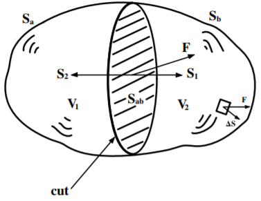
Figure 19.9.1:A volume V enclosed by a closed surface S is cut into two pieces at the surface Sab. This gives V1 enclosed by S1 and V1 enclosed by S2.
Consider the flux Φ of a vector field F for a closed surface, usually called a Gaussian surface, S shown in Figure 19.9.1.
Φ=∮SF⋅dS(H.3)
If the enclosed volume is cut in to two pieces enclosed by surfaces S1=Sa+Sab and S2=Sb+Sab. The flux through the surface Sab common to both S1 and S2 are equal and in the same direction. Then the net flux through the sum of S1 and S2 is given by
∮S1F⋅dS+∮S2F⋅dS=∮SF⋅dS(H.4)
since the contributions of the common surface Sab cancel in that the flux out of S1 is equal and opposite to the flux into S2 over the surface Sab. That is, independent of how many times the volume enclosed by S is subdivided, the net flux for the sum of all the Gaussian surfaces enclosing these subdivisions of the volume, still equals ∮SF⋅dS.
Consider that the volume enclosed by S is subdivided into N subdivisions where N→∞, then even though ∮SiF⋅dS→0 as N→∞, the sum over surfaces of all the infinitesimal volumes remains unchanged
Φ=∮SF⋅dS=i∑N→∞∮SiF⋅dS(H.5)
Thus we can take the limit of a sum of an infinite number of infinitesimal volumes as is needed to obtain a differential form. The surface integral for each infinitesimal volume will equal zero which is not useful, that is ∮SiF⋅dS→0 as N→∞. However, the flux per unit volume has a finite value as N→∞. This ratio is called the divergence of the vector field;
divF=LimΔτi→0Δτi∮SiF⋅dS(H.6)
where Δτi is the infinitesimal volume enclosed by surface Si. The divergence of the vector field is a scalar quantity.
Thus the sum of flux over all infinitesimal subdivisions of the volume enclosed by a closed surface S equals
In the limit N→∞, Δτi→0, this becomes the integral;
Φ=∮SF⋅dS=∫EnclosedvolumedivFdτ(H.8)
This is called the Divergence Theorem or Gauss’s Theorem. To avoid confusion with Gauss’s law in electrostatics, it will be referred to as the Divergence theorem.
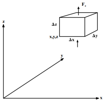
Figure 19.9.2:Computation of flux out of an infinitesimal rectangular box, Δx, Δy, Δz.
Consider the special case of an infinitesimal rectangular box, size Δx,Δy,Δz shown in Figure 19.9.2. Consider the net flux for the z component Fzentering the surface ΔxΔy at location (x,y,z).
ΔΦzin=(Fz+2Δx∂x∂Fz+2Δy∂y∂Fz)ΔxΔy(H.9)
The net flux of the z component out of the surface at z+Δz is
since Δτ=ΔxΔyΔz. But the right hand side of the equation equals the scalar product ∇⋅F, that is,
divF=∇⋅F(H.14)
The divergence is a scalar quantity. The physical meaning of the divergence is that it gives the net flux per unit volume flowing out of an infinitesimal volume. A positive divergence corresponds to a net outflow of flux from the infinitesimal volume at any location while a negative divergence implies a net inflow of flux to this infinitesimal volume.
It was shown that for an infinitesimal rectangular box
ΔΦ=(∂x∂Fx+∂y∂Fy+∂z∂Fz)ΔxΔyΔz=∇⋅FΔτ(H.15)
Integrating over the finite volume enclosed by the surface S gives
Φ=∮SF⋅dS=Enclosedvolume∫∇⋅Fdτ(H.16)
This is another way of expressing the Divergence theorem
Φ=∮SF⋅dS=Enclosedvolume∫divFdτ(H.17)
The divergence theorem, developed by Gauss, is of considerable importance, it relates the surface integral of a vector field, that is, the outgoing flux, to a volume integral of ∇⋅F over the enclosed volume.
Maxwell’s laws relate the circulation of the field around a closed loop to the rate of change of flux through the surface bounded by the closed loop. It is possible to write these integral equations in a differential form as follows.
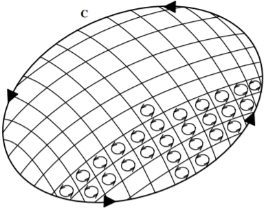
Consider the line integral around a closed loop C shown in Figure 19.9.3.
If this area is subdivided into two areas enclosed by loops C1 and C2, then the sum of the line integrals is the same
∮CF⋅dl=∮C1F⋅dl+∮C2F⋅dl(H.18)
because the contributions along the common boundary cancel since they are taken in opposite directions if C1 and C2 both are taken in the same direction. Note that the line integral, and corresponding enclosed area,
are vector quantities related by the right-hand rule and this must be taken into account when subdividing the area. Thus the area can be subdivided into an infinite number of pieces for which
where ΔSi is the infinitesimal area bounded by the closed sub-loop Ci and ΔSi⋅n is the normal component of this area pointing along the n direction which is the direction along which the line integral points.
Figure 19.9.3:The circulation around a path is equal to the sum of the circulations around subareas made by subdividing the area.
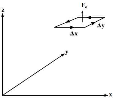
The component of the curl of the vector function along the direction n is defined to be
The physics meaning of the curl is that it is the circulation, or rotation, for an infinitesimal loop at any location. The word curl is German for rotation.
Potential formulations of curl-free and divergence-free fields¶
Interesting consequences result from the Divergence theorem and Stokes Theorem for vector fields that are either curl-free or divergence-free. In particular two theorems result from the second derivatives of a vector field.
everywhere. This is automatically obeyed if the vector field is expressed as the gradient of a scalar field
F=∇ϕ(H.32)
since
∇×(∇ϕ)=0(H.33)
That is, any curl-free vector field can be expressed in terms of the gradient of a scalar field.
The scalar field ϕ is not unique, that is, any constant α can be added to ϕ since ∇α=0, that is, the addition of the constant α does not change the gradient. This independence to addition of a number to the scalar potential is called a gauge invariance discussed in chapter 13.2, for which
F=∇ϕ′=∇(ϕ+α)=∇ϕ(H.34)
That is, this gauge-invariant transformation does not change the observable F. The electrostatic field E and the gravitation field g are examples of irrotational fields that can be expressed as the gradient of scalar potentials.
everywhere. This is automatically obeyed if the field F is expressed in terms of the curl of a vector field G such that
F=∇×G(H.36)
since ∇⋅∇×G=0. That is, any divergence-free vector field can be written as the curl of a related vector field.
As discussed in chapter 13.2, the vector potential G is not unique in that a gauge transformation can be made by adding the gradient of any scalar field, that is, the gauge transformation G′=G+∇φ gives
F=∇×G′=∇×(G+∇φ)=∇×G.(H.37)
This gauge invariance for transformation to the vector potential G′ does not change the observable vector field F. The magnetic field B is an example of a solenoidal field that can be expressed in terms of the curl of a vector potential A.
Any linear system that is subject to a time-dependent forcing function F(t), can be expressed as a linear superposition of frequency-dependent solutions of the individual harmonic decomposition a(ω) of the forcing function. Similarly, any linear system subject to a spatially-dependent forcing function F(x) can be expressed as a linear superposition of the wavenumber-dependent solutions of the individual harmonic decomposition a(kx) of the forcing function. Fourier analysis provides the mathematical procedure for the transformation between the periodic waveforms and the harmonic content, that is, F(t)⇔a(ω), or F(x)⇔a(kx). Fourier’s theorem states that any arbitrary forcing function F(t) can be decomposed into a sum of harmonic terms. For example for a time-dependent periodic forcing function the decomposition can be a cosine series of the form
F(t)=n=1∑∞αncos(nω0t+ϕn)(I.1)
where ω0 is the lowest (fundamental) frequency solution. For an aperiodic function a cosine decomposition can be of the form
F(t)=∫0∞α(ω)cos(ωt+ϕ(ω))dω(I.2)
Either of the complementary functions F(t)⇔a(ω), or F(x)⇔a(kx) are equivalent representations of the harmonic content that can be used to describe signals and waves. The following two sections give an introduction to Fourier analysis.
Discrete solutions occur for systems when periodic boundary conditions exist. The response of periodic systems can be described in either the time versus angular frequency domains, or equivalently, the spatial coordinate x versus the corresponding wave number kx. For periodic systems this decomposition leads to the Fourier series where a generalized phase coordinate ϕ can be used to represent either the time or spatial coordinates, that is, with ϕ=ω0t or ϕ=kxx respectively. The Fourier series relates the two representations of the discrete wave solutions for such periodic systems.
Fourier’s theorem states that for a general periodic system any arbitrary forcing function F(ϕ) can be decomposed into a sum of sinusoidal or cosinusoidal terms. The summation can be represented by three equivalent series expansions given below, where ϕ=ω0t or ϕ=k0⋅r, and where ω0,k0 are the fundamental angular frequency and fundamental wave number respectively.
f(ϕ)=2a0+n=1∑∞[ancos(nϕ)+bnsin(nϕ)](I.3)
f(ϕ)=2a0+n=0∑∞cncos(nϕ+φn)(I.4)
f(ϕ)=2a0+n=0∑∞dnsin(nϕ+θn)(I.5)
where n is an integer, and φn,θn are phase shifts fit to the initial conditions.
The normal modes of a discrete system form a complete set of solutions that satisfy the following orthogonality relation
∫02πfn(ϕ)fm(ϕ)dϕ=cnδmn(I.6)
where δmn is the Kronecker delta symbol defined in equation (9.2.10). Orthogonality can be used to determine the coefficients for equations I.3 to be
a0=π1∫−π+πf(ϕ)dϕ(I.7)
an=π1∫−π+πf(ϕ)cos(nϕ)dϕ(I.8)
bn=π1∫−π+πf(ϕ)sin(nϕ)dϕ(I.9)
Similarly the coefficients for I.4 and I.5 are related to the above coefficients by
cn2=dn2=an2+bn2
Instead of the simple trigonometric form used in equations (I.3 − I.5) the cosine and sine functions can be expanded into the exponential form where
where n is any integer and, from the orthogonality, the Fourier coefficients are given by
gn=2π1∫−π+πf(ϕ)enϕdϕ(I.12)
These coefficients are related to the cosine plus sine series amplitudes by
gn=21(an−ibn)(when n is positive)
gn=21(an+ibn)(when n is negative)
These results show that the coefficients of the exponential series are in general complex, and that they occur in conjugate pairs (that is, the imaginary part of a coefficient an is equal but opposite in sign to that for the coefficient a−n). Although the introduction of complex coefficients may appear unusual, it should be remembered that the real part of a pair of coefficients denotes the magnitude of the cosine wave of the relevant frequency, and that the imaginary part denotes the magnitude of the sine wave. If a particular pair of coefficients an and a−n are real, then the component at the frequency nω0 is simply a cosine; if an and a−n are purely imaginary, the component is just a sine; and if, as is the general case, an and a−n are complex, both cosine and a sine terms are present.
The use of the exponential form of the Fourier series gives rise to the notion of ‘negative frequency’. Of course, f(t)=ancosωnt is a wave of a single frequency ωn=nω0 radians/second, and may be represented by a single line of height an in a normal spectral diagram. However, using the exponential form of the Fourier series results in both positive and negative ω components.
The coexistence of both negative and positive angular frequencies ±ω can be understood by consideration of the Argand diagram where the real component is plotted along the x-axis and the imaginary component along the y-axis. The function gne+iωt represents a vector of length gn that rotates with an angular velocity ω in a positive direction, that is counterclockwise, whereas, gne−iωt represents the vector rotating in a negative direction, that is clockwise. Thus the sum of the two rotating vectors, according to equations I.3, leads to cancellation of the opposite components on the imaginary y axis and addition of the two gncosωt real components on the x axis. Subtraction leads to cancellation of the real x components and addition of the imaginary y axis components.
The Fourier transform (also called the Fourier integral) does for the non-repetitive signal waveform what the Fourier series does for the repetitive signal. It was shown that the line spectrum of a recurrent periodic pulse waveform is modified as the pulse duration decreases, assuming the period of the waveform (and hence its fundamental component) remains unchanged. Suppose now that the duration of the pulses remain fixed but the separation between them increases, giving rise to an increasing period. In the limit, only a single rectangular pulse remains, its neighbors having moved away on either side towards ±∞. In this case, the fundamental frequency ω0 tends towards zero and the harmonics become extremely closely spaced and of vanishingly small amplitudes, that is, the system approximates a continuous spectrum.
Mathematically, this situation may be expressed by modifications to the exponential form of the Fourier series already derived. Let the phase factor ϕ=ω0t in Equation I.11 then
Equation I.15 shows how a non-repetitive time-domain wave form is related to its continuous spectrum. These are known as Fourier integrals or Fourier transforms. They are of central importance for signal processing. For convenience the transforms often are written in the operator formalism using the F symbol in the form
f(t)=2π1∫−∞+∞G(ω)eiωtdω≡F−1[2π1G(ω)](I.16)
G(ω)=∫−∞+∞f(t)e−iωtdt≡Ff(t)(I.17)
It is very important to grasp the significance of these two equations. The first tells us that the Fourier transform of the waveform f(t) is continuously distributed in the frequency range between ω=±∞, whereas the second shows how, in effect, the waveform may be synthesized from an infinite set of exponential functions of the form e±iωt, each weighted by the relevant value of G(ω). It is crucial to realize that this transformation can go either way equally, that is, from G(ω) to f(t) or vice versa.[2]
An alternative approach for unloosing periodic signals, that is complementary to the Fourier analysis harmonic decomposition, is time-sampled (discrete-sample) waveform analysis where the signal amplitude is measured repetitively at regular time intervals in a time-ordered sequence, that is, a sequence of samples of the instantaneous delta-function amplitudes is recorded. Typically an amplitude-to-digital converter is used to digitize the amplitude for each measured sample and the digital numbers are recorded; this process is called digital signal processing.
The general principles are best explained by first considering the response of a linear system to a step function impulse, followed by a square impulse, and leading to the response of a δ-function impulsive driving force.
Figure 19.10.1:Response of a underdamped linear oscillator with ω=10, and Γ=2 to the following impulsive force. (a) Step function force F=0 for t<0 and F=m for t>0. (b) Square-wave force where F=m for 0<t<τ for τ=3, and F=0 at other times. (c) Delta-function impulse P=1.
where ω1≡ω02−(2Γ)2. This functional form is shown in Figure 19.10.1a. Note that the amplitude of the transient response equals −a at t=0 to cancel the particular solution when it jumps to +a. The oscillatory behavior then is just that of the transient response.
A square impulse can be generated by the superposition of two opposite-sign stepfunctions separated by a time τ as shown in Figure 19.10.1b.
The square impulse can be taken to the limit where the width τ is negligibly small relative to the response times of the system. It can be shown that letting τ→0, but keeping the magnitude of the total impulse P=aτ finite for the impulse at time t0, leads to the solution for the δ-function impulse occurring at t0
x(t)=ω1Pe−2Γ(t−t0)sinω1(t−t0)t>t0(I.22)
This response to a delta function impulse is shown in Figure 19.10.1c for the case where t0=0. An example is the response when the hammer strikes a piano string at t=0.
Figure 19.10.2:Decomposition of the function x(t)=2sin(t)+sin(5t)+31sin(15t)+51sin(25t) into a time-ordered sequence of δ-function samples.
The response of the linearly-damped linear oscillator to an delta function impulse, that has been expressed above, can be used to exploit the powerful Green’s technique for decomposition of any general forcing function. That is, if the driven system is linear, then the principle of superposition is applicable and allowing expression of the inhomogeneous part of the differential equation as the sum of individual delta functions. That is;
x¨+Γx˙+ω02x=n=−∞∑∞mFn(t)=n=−∞∑∞In(t)(I.23)
As illustrated in Figure 19.10.2 discrete-time waveform analysis involves repeatedly sampling the instantaneous amplitude in a regular and repetitive sequence of δ-function impulses. Since the superposition principle applies for this linear system then the waveform can be described by a sum of an ordered series of deltafunction impulses where t′ is the time of an impulse. Integrating over all the δ-function responses that have occurred at time t′, that is prior to the time of interest t, leads to
Superposition allows the summed response of the system to be written in an integral form
x(t)=∫−∞tF(t′)G(t−t′)dt′(I.26)
which gives the final time dependence of the forced system. This repetitive time-sampling approach avoids the need of using Fourier analysis. Note that the Green’s function G(t−t′) includes implicitly the frequency of the free undamped linear oscillator ω0, the free damped linear oscillator ω1≡ω02−(2Γ)2, as well as the damping coefficient Γ. Access to the combination of fast microcomputers coupled to fast digital sampling techniques has made digital signal sampling the pre-eminent technique for signal recording of audio, video, and detector signal processing.
[1] SELECTION OF TEXTBOOKS ON CLASSICAL MECHANICS¶
[Ar78] V. I. Arnold, “Mathematical methods of Classical Mechanics”, 2nd edition, Springer-Verlag (1978)
This textbook provides an elegant and advanced exposition of classical mechanics expressed in the language of differential topology.
[Co50] H.C. Corben and P. Stehle, “Classical Mechanics”, John Wiley (1950)
This classic textbook covers the material at the same level and comparable scope as the present textbook.
[Fo05] G. R. Fowles, G. L. Cassiday, “Analytical Mechanics”. Thomson Brookes/Cole, Belmont, (2005)
An elementary undergraduate text that emphasizes computer simulations.
[Go50] H. Goldstein, “Classical Mechanics”, Addison-Wesley, Reading (1950)
This has remained the gold standard graduate textbook in classical mechanics since 1950. Goldstein’s book is the best graduate-level reference to supplement the present textbook. The lack of worked examples is an impediment to using Goldstein for undergraduate courses. The 3rd edition, published by Goldstein, Poole, and Safko (2002), uses the symplectic notation that makes the book less friendly to undergraduates. The Cline book adopts the nomenclature used by Goldstein to provide a consistent presentation of the material.
[Gr06] R. D. Gregory, “Classical Mechanics”, Cambridge University Press
This outstanding, and original, introduction to analytical mechanics was written by a mathematician. It is ideal for the undergraduate, but the breadth of the material covered is limited.
[Gr10] W. Greiner, “Classical Mechanics, Systems of particles and Hamiltonian Dynamics”, 2nd edition, Springer (2010). This excellent modern graduate textbook is similar in scope and approach to the present text. Greiner includes many interesting worked examples, as well as a reproduction of the Struckmeier[Str08] presentation of the extended Lagrangian and Hamiltonian mechanics formalism of Lanczos[La49].
[Jo98] J. V. José and E. J. Saletan, “Classical Dynamics, A Contemporary Approach”, Cambridge University Press (1998)
This modern advanced graduate-level textbook emphasizes configuration manifolds and tangent bundles which makes it unsuitable for use by most undergraduate students.
[Jo05] O. D. Johns, “Analytical Mechanics for Relativity and Quantum Mechanics”, 2nd edition, Oxford University Press (2005). Excellent modern graduate text that emphasizes the Lanczos[La49] parametric approach to Special Relativity. The Johns and Cline textbooks were developed independently but are similar in scope and approach. For consistency, the name “generalized energy”, which was introduced by Johns, has been adopted in the Cline textbook.
[Ki85] T.W.B. Kibble, F.H. Berkshire. “Classical Mechanics, (5th edition)”, Imperial College Press, London, 2004. Based on the textbook written by Kibble that was published in 1966 by McGrawHill. The 4th and 5th editions were published jointly by Kibble and Berkshire. This excellent and well-established textbook addresses the same undergraduate student audience as the present textbook. This book covers the variational principles and applications with minimal discussion of the philosophical implications of the variational approach.
[La10] O.L. De Lange and J. Pierrus, “Solved Problems in Classical Mechanics”, Oxford University Press, 2010. Presents both numerical and analytical solution of problems in classical mechanics.
[La49] C. Lanczos, “The Variational Principles of Mechanics”, University of Toronto Press, Toronto, (1949)
An outstanding graduate textbook that has been one of the founding pillars of the field since 1949. It gives an excellent introduction to the philosophical aspects of the variational approach to classical mechanics, and introduces the extended formulations of Lagrangian and Hamiltonian mechanics that are applicable to relativistic mechanics.
[La60] L. D. Landau, E. M. Lifshitz, “Mechanics”, Volume 1 of a Course in Theoretical Physics, Pergamon Press (1960)
An outstanding, succinct, description of analytical mechanics that is devoid of any superfluous text. This Course in Theoretical Physics is a masterpiece of scientific writing and is an essential component of any physics library. The compactness and lack of examples makes this textbook less suitable for most undergraduate students.
[Li94] Yung-Kuo Lim, “Problems and Solutions on Mechanics” (1994)
This compendium of 408 solved problems, which are taken from graduate qualifying examinations in physics at several U.S. universities, provides an invaluable resource that complements this textbook for study of Lagrangian and Hamiltonian mechanics.
[Ma65] J. B. Marion, “Classical Dynamics of Particles and Systems”, Academic Press, New York, (1965)
This excellent undergraduate text played a major role in introducing analytical mechanics to the undergraduate curriculum. It has an outstanding collection of challenging problems. The 5th edition has been published by S. T. Thornton and J. B. Marion, Thomson, Belmont, (2004).
[Me70] L. Meirovitch, “Methods of Analytical Dynamics”, McGraw-Hill New York, (1970)
An advanced engineering textbook that emphasizes solving practical problems, rather than the underlying theory.
[Mu08] H. J. W. Müller-Kirsten, “Classical Mechanics and Relativity”, World Scientific, Singapore, (2008)
This modern graduate-level textbook emphasizes relativistic mechanics making it an excellent complement to the present textbook.
[Pe82] I. Percival and D. Richards, “Introduction to Dynamics” Cambridge University Press, London, (1982)
Provides a clear presentation of Lagrangian and Hamiltonian mechanics, including canonical transformations, Hamilton-Jacobi theory, and action-angle variables.
[Sy60] J.L. Synge, “Principles of Classical Mechanics and Field Theory”, Volume III/I of “Handbuch der Physik” Springer-Verlag, Berlin (1960).
A classic graduate-level presentation of analytical mechanics.
[Th04] S.T. Thornton, and J. B. Marion, “Classical Dynamics of Particles and Systems”, 5th edition. Brooks/Cole-Thomson Learning, New York, (2004)
Thornton has expanded the outstanding collection of challenging problems in this popular classical mechanics book.
The only asymmetry in the Fourier transform relations comes from the 2π factor originating from the fact that by convention physicists use the angular frequency ω=2πν rather than the frequency ν. In order to restore symmetry many papers use the factor 2π1 in both relations rather than using the 2π1 factor in Equation I.16 and unity in Equation I.17.