16.1: Introduction
Lagrangian and Hamiltonian mechanics have been used to determine the equations of motion for discrete systems having a finite number of discrete variables where . There are important classes of systems where it is more convenient to treat the system as being continuous. For example, the interatomic spacing in solids is a few which is negligible compared with the size of typical macroscopic, three-dimensional solid objects. As a consequence, for wavelengths much greater than the atomic spacing in solids, it is useful to treat macroscopic crystalline lattice systems as continuous three-dimensional uniform solids, rather than as three-dimensional discrete lattice chains. Fluid and gas dynamics are other examples of continuous mechanical systems. Another important class of continuous systems involves the theory of fields, such as electromagnetic fields. Lagrangian and Hamiltonian mechanics of the continua extend classical mechanics into the advanced topic of field theory. This chapter goes beyond the scope of a typical undergraduate classical mechanics course in order to provide a brief glimpse of how Lagrangian and Hamiltonian mechanics can underlie advanced and important aspects of the mechanics of the continua, including field theory.

Figure 16.1.1:Rubber bands are one type of elastic solid that can be described with continuous formalism. (CC BY-SA 3.0; Bill Ebbesen)
16.2: The Continuous Uniform Linear Chain
The Lagrangian for the discrete lattice chain, for longitudinal modes, is given by equation to be
where the masses are attached in series to identical springs of length and spring constant . Assume that the spring has a uniform cross-section area and length . Then each spring volume element has a mass , that is, the volume mass density or . Chapter 16.5 will show that the spring constant where is Young’s modulus, is the cross sectional area of the chain element, and is the length of the element. Then the spring constant can be written as . Therefore Equation 16.1 can be expressed as a sum over volume elements
In the limit that and the spacing , then the summation in Equation 16.2 can be written as a volume integral where is the distance along the linear chain and the volume element . Then the Lagrangian can be written as the integral over the volume element rather than a summation over . That is,
The discrete-chain coordinate is assumed to be a continuous function for the uniform chain. Thus the integral form of the Lagrangian can be expressed as
where the function is called the Lagrangian density defined by
The variable in the Lagrangian density is not a generalized coordinate; it only serves the role of a continuous index played previously by the index . For the discrete case, each value of defined a different generalized coordinate . Now for each value of there is a continuous function which is a function of both position and time.
Lagrange’s equations of motion applied to the continuous Lagrangian in Equation 16.4 gives
This is the familiar wave equation in one dimension for a longitudinal wave on the continuous chain with a phase velocity
The continuous linear chain also can exhibit transverse modes which have a Lagrangian density were the Young’s modulus is replaced by the tension in the chain, and is replaced by the linear mass density of the chain, leading to a phase velocity for a transverse wave .
16.3: The Lagrangian density formulation for continuous systems
One spatial dimension
In general the Lagrangian density can be a function of , and . It is of interest that Hamilton’s principle leads to a set of partial differential equations of motion, based on the Lagrangian density, that are analogous to the Lagrange equations of motion for discrete systems. When deriving the Lagrangian equations of motion in terms of the Lagrangian density using Hamilton’s principle, the notation is simplified if the system is limited to one spatial coordinate . In addition, it is convenient to use the compact notation where the spatial derivative is written and the time derivative is , and the one-dimensional Lagrangian density is assumed to be a function . The appearance of the derivative as an argument of the Lagrange density is a consequence of the continuous dependence of on . In principle, higher-order derivatives could occur but they do not arise in most problems of physical interest.
Assuming that the one spatial dimension is , then Hamilton’s principle of least action can be expressed in terms of the Lagrangian density as
Following the same approach used in chapter 5.2, it is assumed that the stationary path for the action integral is described by the function . Define a neighboring function using a parametric representation such that when , the extremum function yields the stationary action integral .
Assume that an infinitesimal fraction of a neighboring function is added to the extremum path . That is, assume
where it is assumed that both the extremum function and the auxiliary function are well behaved functions of and , with continuous first derivatives, and that at and because, for all possible paths, the function must be identical with at the end points of the path, i.e. .
A parametric family of curves , as a function of the admixture coefficient , is described by the function
Then Hamilton’s principle requires that the action integral be a stationary function value for , that is, is independent of which is satisfied if
Equations 16.9, 16.10,and 16.11 give the partial differentials
Integration by parts in both the and terms in Equation 16.13, plus using the fact that at both end points, yields
Therefore Hamilton’s principle, Equation 16.13 becomes
Since the auxiliary function is arbitrary, then the integrand term in the square brackets of Equation 16.19 must equal zero. That is,
Equation 16.20 gives the equations of motion in terms of the Lagrangian density that has been derived based on Hamilton’s principle.
Three spatial dimensions
Equation expresses the Lagrangian as an integral of the Lagrangian density over a single continuous index where the Lagrangian density is a function . The derivation of the Lagrangian equations of motion in terms of the Lagrangian density for three spatial dimensions involves the straightforward addition of the , and coordinates. That is, in three dimensions the vector displacement is expressed by the vector and the Lagrangian density is related to the Lagrangian by integration over three dimensions. That is, they are related by the equation
where, in cartesian coordinates, the volume element . The Lagrangian density is a function where the one field quantity has been extended to a spatial vector and the spatial derivatives have been transformed into . Applying the method used for the one-dimensional spatial system, to the three-dimensional system, leads to the following set of equations of motion
where the spatial derivatives have been written explicitly for clarity.
Note that the equations of motion, Equation 16.22, treat the spatial and time coordinates symmetrically. This symmetry between space and time is unchanged by multiplying the spatial and time coordinate by arbitrary numerical factors. This suggests the possibility of introducing a four-dimensional coordinate system
where the parameter is freely chosen. Using this 4-dimensional formalism allows Equation 16.22 to be written more compactly as
As discussed in chapter 17, relativistic mechanics treats time and space symmetrically, that is, a four-dimensional vector can be used that treats time and the three spatial dimensions symmetrically and equally. This four-dimensional space-time formulation allows the first four terms in Equation 16.22 to be condensed into a single term which illustrates the symmetry underlying Equation 16.23. If the Lagrangian density is Lorentz invariant, and if , then Equation 16.23 is covariant. Thus the Lagrangian density formulation is ideally suited to the development of relativistically covariant descriptions of fields.
16.4: The Hamiltonian density formulation for continuous systems
Chapter 16.3 illustrated, in general terms, how field theory can be expressed in a Lagrangian formulation via use of the Lagrange density. It is equally possible to obtain a Hamiltonian formulation for continuous systems analogous to that obtained for discrete systems. As summarized in chapter 8, the Hamiltonian and Hamilton’s canonical equations of motion are related directly to the Lagrangian by use of a Legendre transformation. The Hamiltonian is defined as being
The generalized momentum is defined to be
Equation 16.25 allows the Hamiltonian 16.24 to be written in terms of the conjugate momenta as
where the Lagrangian has been partitioned into the terms for each of the individual coordinates, that is, .
In the limit that the coordinates are continuous, then the summation in Equation 16.26 can be transformed into a volume integral over the Lagrangian density . In addition, a momentum density can be represented by the vector field where
Then the obvious definition of the Hamiltonian density is
where the Hamiltonian density is defined to be
Unfortunately the Hamiltonian density formulation does not treat space and time symmetrically making it more difficult to develop relativistically covariant descriptions of fields. Hamilton’s principle can be used to derive the Hamilton equations of motion in terms of the Hamiltonian density analogous to the approach used to derive the Lagrangian density equations of motion. As described in Classical Mechanics edition by Goldstein, the resultant Hamilton equations of motion for one dimension are
Note that Equation 16.31 differs from that for discontinuous systems.
16.5: Linear Elastic Solids
Elasticity is a property of matter where the atomic forces in matter act to restore the shape of a solid when distorted due to the application of external forces. A perfectly elastic material returns to its original shape if the external force producing the deformation is removed. Materials are elastic when the external forces do not exceed the elastic limit. Above the elastic limit, solids can exhibit plastic flow and concomitant heat dissipation. Such non-elastic behavior in solids occurs when they are subject to strong external forces.
The discussion of linear systems, in chapters 3 and 14, focused on one dimensional systems, such as the linear chain, where the transverse rigidity of the chain was ignored. An extension of the one-dimensional linear chain to two-dimensional membranes, such as a drum skin, is straightforward if the membrane is thin enough so that the rigidity of the membrane can be ignored. Elasticity for three-dimensional solids requires accounting for the strong elastic forces exerted against any change in shape in addition to elastic forces opposing change in volume. The stiffness of solids to changes in shape, or volume, is best represented using the concepts of stress and strain.
Forces in matter can be divided into two classes;
body forces, such as gravity, which act on each volume element, and
surface forces which are the forces that act on both sides of any infinitesimal surface element inside the solid.
Surface forces can have components along the normal to the infinitesimal surface, as well as shear components in the plane of the surface element. Typically solids are elastic to both normal and shear components of the surface forces whereas shear forces in liquids and gases lead to fluid flow plus viscous forces due to energy dissipation. As described below, the forces acting on an infinitesimal surface element are best expressed in terms of the stress tensor, while the relative distortion of the shape, or volume, of the body are best expressed in terms of the strain tensor. The moduli of elasticity relate the ratio of the corresponding stress and strain tensors. The moduli of elasticity are constant in linear elastic solids and thus the stress is proportional to the strain providing that the strains do not exceed the elastic limit.
Stress tensor
Consider an infinitesimal surface area of an arbitrary closed volume element inside the medium. The surface area element is defined as a vector where is the outward normal to the closed surface that encloses the volume element. Assume that is the force element exerted by the outside on the material inside the volume element. The stress tensor is defined as the ratio of and where the force vector is given by the inner product of the stress tensor and the surface element vector . That is,
Since both and are vectors, then Equation 16.33 implies that the stress tensor must be a second-rank tensor as described in appendix 19.5, that is, the stress tensor is analogous to the rotation matrix or the inertia tensor. Note that if and are collinear, then the stress tensor reduces to the conventional pressure . The general stress tensor equals the momentum flux density and has the dimensions of pressure.
Strain tensor
Forces applied to a solid body can lead to translational, or rotational acceleration, in addition to changing the shape or volume of the body. Elastic forces do not act when an overall displacement of an infinitesimal volume occurs, such as is involved in translational or rotational motion. Elastic forces act to oppose position-dependent differences in the displacement vector , that is, the strain depends on the tensor product . For an elastic medium, the strain depends only on the applied stress and not on the prior loading history.
Consider that the matter at the location is subject to an elastic displacement , and similarly at a displaced location where are cartesian coordinates. The net relative displacement between and is given by
Ignoring the second order term equation gives that the component of is
Define the elements of the strain tensor to be given by
then
Thus the strain tensor is a rank-2 tensor defined as the ratio of the strain vector and the infinitesimal area vector .
where the component form of the rank -2 strain tensor is
The potential-energy density for linear elastic forces is quadratic in the strain components. That is, it is of the form
where is a rank-4 tensor. No preferential directions remain for a homogeneous isotropic elastic body which allows for two contractions, thereby reducing the potential energy density to the inner product
Moduli of elasticity
The modulus of elasticity of a body is defined to be the slope of the stress-strain curve and thus, in principle, it is a complicated rank-4 tensor that characterizes the elastic properties of a material. Thus the general theory of elasticity is complicated because the elastic properties depend on the orientation of the microscopic composition of the elastic matter. The theory simplifies considerably for homogeneous, isotropic linear materials below the elastic limit, where the strain is proportional to the applied stress. That is, the modulus of elasticity then reduces by contractions to a constant scalar value that depends on the properties of the matter involved.
The potential energy density for homogeneous, isotropic, linear material, Equation 16.41, can be separated into diagonal and off-diagonal components of the strain tensor. That is,
The diagonal first term is the dilation term which corresponds to changes in the volume with no changes in shape. The off-diagonal second term involves the shear terms that correspond to changes of the shape of the body that also changes the volume. The constants and are Lamé’s moduli of elasticity which are positive. The various moduli of elasticity, corresponding to different distortions in the shape and volume of any solid body, can be derived from Lamé’s moduli for the material.
The components of the elastic forces can be derived from the gradient of the elastic potential energy, Equation 16.42 by use of Gauss’ law plus vector differential calculus. The components of the elastic force, derived from the strain tensor , can be associated with the corresponding components of the stress tensor . Thus, for homogeneous isotropic linear materials, the components of the stress tensor are related to the strain tensor by the relation
where it has been assumed that . The two moduli of elasticity and are material-dependent constants. Equation 16.43 can be written in tensor notation as
where is the trace of the strain tensor and is the identity matrix.
Equation 16.44 can be inverted to give the strain tensor components in terms of the stress tensor components.
The various moduli of elasticity relate combinations of different stress and strain tensor components. The following five elastic moduli are used frequently to describe elasticity in homogeneous isotropic media, and all are related to Lamé’s two moduli of elasticity.
Young’s modulus describes tensile elasticity which is axial stiffness of the length of a body to deformation along the axis of the applied tensile force.
2)Bulk modulus defines the relative dilation or compression of a bodies volume to pressure applied uniformly in all directions.
The bulk modulus is an extension of Young’s modulus to three dimensions and typically is larger than . The inverse of the bulk modulus is called the compressibility of the material.
Shear modulus describes the shear stiffness of a body to volume-preserving shear deformations. The shear strain becomes a deformation angle given by the ratio of the displacement along the axis of the shear force and the perpendicular moment arm. The shear modulus equals Lamé’s constant . That is,
Poisson’s ratio is the negative ratio of the transverse to axial strain. It is a measure of the volume conserving tendency of a body to contract in the directions perpendicular to the axis along which it is stretched. In terms of Lamé’s constants, Poisson’s ratio equals
Note that for a stable, isotropic elastic material, Poisson’s ratio is bounded between to ensure that the , and moduli have positive values. At the incompressible limit, , and the bulk modulus and Lame parameter are infinite, that is, the compressibility is zero. Typical solids have Poisson’s ratios of if hard and if soft.
The stiffness of elastic solids in terms of the elastic moduli of solids can be complicated due to the geometry and composition of solid bodies. Often it is more convenient to express the stiffness in terms of the spring constant where
The spring constant is inversely proportional to the length of the spring because the strain of the material is defined to be the fractional deformation, not the absolute deformation.
16.5.4 Equations of motion in a uniform elastic media
The divergence theorem relates the volume integral of the divergence of to the vector force density acting on the closed surface.
That is, the inner product of the del operator, , and the rank-2 stress tensor , give the vector force density . This force acting on the enclosed mass , for the closed volume, leads to an acceleration . Thus
Use Equation 16.44 to relate the stress tensor to the moduli of elasticity gives
where . In general this equation is difficult to solve. However, for the simple case of a plane wave in the direction, the problem reduces to the following three equations
Equation 16.54 corresponds to a longitudinal wave traveling with velocity . Equations 16.55, 16.56 correspond to two perpendicular transverse waves traveling with velocity . This illustrates the important fact that longitudinal waves travel faster than transverse waves in an elastic solid. Seismic waves in the Earth, generated by earthquakes, exhibit this property. Note that shearing stresses do not exist in ideal liquids and gases since they cannot maintain shear forces and thus .
16.6: Electromagnetic Field Theory
Maxwell stress tensor
Analytical formulations for continuous systems, developed for describing elasticity, are generally applicable when applied to other fields, such as the electromagnetic field. The use of the Maxwell’s stress tensor , to describe momentum in the electromagnetic field, is an important example of the application of continuum mechanics in field theory.
The Lorentz force can be written as
where the force density is defined to be
Maxwell’s equations
can be used to eliminate the charge and current densities in Equation 16.57
Vector calculus gives that
while Faraday’s law gives
Equation 16.62 allows Equation 16.61 to be rewritten as
Equation 16.63 can be inserted into Equation 16.60. In addition, a term can be added since which allows equation 16.60 to be written in the symmetric form
Using the vector identity
Let , then
That is
Similarly
Inserting equations 16.68 and 16.69 into Equation 16.65 gives
This complicated formula can be simplified by defining the rank-2 Maxwell stress tensor which has components
The inner product of the del operator and the Maxwell stress tensor is a vector with components of
The above definition of the Maxwell stress tensor, plus the Poynting vector , allows the force density Equation 16.58 to be written in the form
The divergence theorem allows the total force, acting of the volume , to be written in the form
Note that, if the Poynting vector is time independent, then the second term in Equation 16.75 is zero and the Maxwell stress tensor is the force per unit area, (stress) acting on the surface. The fact that is a rank-2 tensor is apparent since the stress represents the ratio of the force-density vector and the infinitesimal area vector , which do not necessarily point in the same directions.
Momentum in the electromagnetic field
Chapter 7.2 showed that the electromagnetic field carries a linear momentum where is the charge on a body and is the electromagnetic vector potential. It is useful to use the Maxwell stress tensor to express the momentum density directly in terms of the electric and magnetic fields.
Newton’s law of motion can be used to write Equation 16.75 as
where is the total mechanical linear momentum of the volume . Equation 16.76 implies that the electromagnetic field carries a linear momentum
The term in Equation 16.76 is the momentum per unit time flowing into the closed surface. In field theory it can be useful to describe the behavior in terms of the momentum flux density . Thus the momentum flux density in the electromagnetic field is
Then Equation 16.76 implies that the total momentum flux density is related to Maxwell’s stress tensor by
That is, like the elasticity stress tensor, the divergence of Maxwell’s stress tensor equals the rate of change of the total momentum density, that is, is the momentum flux density.
This discussion of the Maxwell stress tensor and its relation to momentum in the electromagnetic field illustrates the role that analytical formulations of classical mechanics can play in field theory
16.7: Ideal Fluid Dynamics
The distinction between a solid and a fluid is that a fluid flows under shear stress whereas the elasticity of solids oppose distortion and flow. Shear stress in a fluid is opposed by dissipative viscous forces, which depend on velocity, as opposed to elastic solids where the shear stress is opposed by the elastic forces which depend on the displacement. An ideal fluid is one where the viscous forces are negligible, and thus the shear stress Lamé parameter .
Continuity Equation
Fluid dynamics requires a different philosophical approach than that used to describe the motion of an ensemble of known solid bodies. The prior discussions of classical mechanics used, as variables, the coordinates of each member of an ensemble of particles with known masses. This approach is not viable for fluids which involve an enormous number of individual atoms as the fundamental bodies of the fluid. The best philosophical approach for describing fluid dynamics is to employ continuum mechanics using definite fixed volume elements and describe the fluid in terms of macroscopic variables of the fluid such as mass density , pressure , and fluid velocity .
Conservation of fluid mass requires that the rate of change of mass in a fixed volume must equal the net inflow of mass.
Using the divergence theorem allows this to be written as
Mass conservation must hold for any arbitrary volume, therefore the continuity equation can be written in the differential form
Euler’s hydrodynamic equation
The fluid surrounding a volume exerts a net force that equals the surface integral of the pressure . This force can be transformed to a volume integral of . The net force then will lead to an acceleration of the volume element. That is
Thus the force density is given by
Note that the acceleration in Equation 16.83 refers to the rate of change of velocity for individual atoms in the fluid, not the rate of change of fluid velocity at a fixed point in space. These two accelerations are related by noting that, during the time , the change in velocity of a given fluid particle is composed of two parts, namely
the change during in the velocity at a fixed point in space, and
the difference between the velocities at that same instant in time at two points displaced a distance apart, where is the distance moved by a given fluid particle during the time .
The first part is given by at a given point in space. The second part equals
Thus
Divide both sides by gives that the acceleration of the atoms in the fluid equals
Substitute Equation 16.87 into 16.84 gives
This is Euler’s equation for hydrodynamics. The two terms on the left represent the acceleration in the individual fluid components while the right-hand side lists the force density producing the acceleration.
Additional forces can be added to the right-hand side. For example, the gravitational force density can be expressed in terms of the gravitational scalar potential to be
Inclusion of the gravitational field force density in Euler’s equation gives
Irrotational flow and Bernoulli’s equation
Streamlined flow corresponds toirrotational flow, that is, . Since irrotational flow is curl free, the velocity streamlines can be represented by a scalar potential field . That is
This scalar potential field can be used to derive the vector velocity field for irrotational flow.
Note that the term in Euler’s Equation 16.90 can be rewritten using the vector identity
Inserting Equation 16.92 into Euler’s Equation 16.90 then gives.
Potential flow corresponds to time independent irrotational flow, that is, both and . For potential flow Equation 16.93 reduces to
which implies that
This is the famous Bernoulli’s equation that relates the interplay of the fluid velocity, pressure and gravitational energy. Bernoulli’s equation plays important roles in both hydrodynamics and aerodynamics.
Gas flow
Fluid dynamics applied to gases is a straightforward extension of fluid dynamics that employs standard thermodynamical concepts. The following example illustrates the application of fluid mechanics for calculating the velocity of sound in a gas.
16.8: Viscous Fluid Dynamics
Viscous fluid dynamics is a branch of classical mechanics that plays a pivotal role in a wide range of aspects of life, such as blood flow in human anatomy, weather, hydraulic engineering, and transportation by land, sea, and air. Viscous fluid flow provides nature’s most common manifestation of nonlinearity and turbulence in classical mechanics, and provides an excellent illustration of possible solutions of non-linear equations of motion introduced in chapter 4. A detailed description of turbulence remains a challenging problem and this subject has the reputation of being the last great unsolved problem in classical mechanics. There is an apocryphal story that Werner Heisenberg was asked, if given the opportunity, what would he like to ask God. His reply was “When I meet God, I am going to ask him two questions: Why relativity? and why turbulence?, I really believe he will only have an answer to the first”.
In contrast to solids, fluids do not have elastic restoring forces to support shear stress because the fluid flows. Shear stresses in fluids are balance by viscous forces which are velocity dependent. There are two mechanisms that lead to shear stress acting between adjacent fluid layers in relative motion. The first mechanism involves laminar flow where the viscous forces produce shear stress between adjacent layers of the fluid which are moving parallel along adjacent streamlines at differing velocities. Viscous forces typically dominate laminar flow. High viscosity fluids like honey exhibit laminar flow and are more difficult to stir or pour compared with low-viscosity fluids like water. The second mechanism involves turbulent flow where shear stress is due to momentum transfer between adjacent layers when the flow breaks up into large-scale coherent vortex structures which carry most of the kinetic energy. These eddies lead to transverse motion that transfers momentum plus heat between adjacent layers and leads to higher drag. The wing-tip vortex produced by the wing tip of an aircraft is an example of a dynamically-distinct, large-scale, coherent vortex structure which has considerable angular momentum and decays by fragmentation into a cascade of smaller scale structures.
Navier-Stokes equation
Viscous forces acting on the small-scale coherent structures eventually dissipate the energy in turbulent motion. The viscous drag can be handled in terms of a stress tensor analogous to its use when accounting for the elastic restoring forces in elasticity as discussed in chapter 16.5.3. That is, the viscous force density is related to the deceleration of the volume element by
where the components of the stress tensor are
Note that the stress tensor gives the momentum flux density tensor, which involves a diagonal term proportional to pressure , plus a viscous drag term that is proportional to the product of two velocities.
The Navier-Stokes equations are the fundamental equations characterizing fluid flow. They are based on application of Newton’s second law of motion to fluids together with the assumption that the fluid stress is the sum of a diffusing viscous term plus a pressure term. Combining Euler’s equation, , with 16.95 gives the Navier-Stokes equation
where is the fluid density, is the flow velocity vector, the pressure, is the shear stress tensor viscous drag term, and represents external body forces per unit volume such as gravity acting on the fluid. For incompressible flow the stress tensor term simplifies to . Then the Navier-Stokes equation simplifies to
where is the viscosity drag term. The left-hand side of Equation 16.98 represents the rate of change of momentum per unit volume while the right-hand side represents the summation of the forces per unit volume that are acting.
The Navier-Stokes equations are nonlinear due to the term as well as being a function of velocity. This non-linearity leads to a wide spectrum of dynamic behavior ranging from ordered laminar flow to chaotic turbulence. Numerical solution of the Navier-Stokes equations is extremely difficult because of the wide dynamic range of the dimensions of the coherent structures involved in turbulent motion. For example, simulation calculations require use of a high resolution mesh which is a challenge to the capabilities of current generation computers.
The microscopic boundary condition at the interface of the solid and fluid is that the fluid molecules have zero average tangential velocity relative to the normal to the solid-fluid interface. This implies that there is a boundary layer for which there is a gradient in the tangential velocity of the fluid between the solid-fluid interface and the free-steam velocity. This velocity gradient produces vorticity in the fluid. When the viscous forces are negligible then the angular momentum in any coherent vortex structure is conserved leading to the vortex motion being preserved as it propagates.
Reynolds number
Fluid flow can be characterized by the Reynolds number Re which is a dimensionless number that is a measure of the ratio of the inertial forces to viscous forces . That is,
where is the relative velocity between the free fluid flow and the solid surface, is a characteristic linear dimension, is the dynamic viscosity of the fluid, is the kinematic viscosity , and is the density of the fluid. The Law of Similarity implies that at a given Reynolds number, for a specific shaped solid body, the fluid flow behaves identically independent of the size of the body. Thus one can use small models in wind tunnels, or water-flow tanks, to accurately model fluid flow that can be scaled up to a full-sized aircraft or boats by scaling and to give the same Reynolds number.
Laminar and turbulent fluid flow
Fluid flow over a cylinder illustrates the general features of fluid flow. The drag force acting on a cylinder of diameter and length , with the cylindrical axis perpendicular to the fluid flow, is given by
where is the coefficient of drag. Figure 16.8.1 upper shows the dependence of the drag coefficient as a function of the Reynolds number, for fluid flow that is transverse to a smooth circular cylinder. The lower part of Figure 16.8.1 shows the streamlines for flow around the cylinder at various Reynolds numbers for the points identified by the letters , , , , and on the plot of the drag coefficient versus Reynolds number for a smooth cylinder.
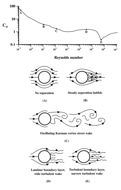
Figure 16.8.1:Upper: The dependence of the coefficient of drag on Reynolds number Re for fluid flow perpendicular to a smooth circular cylinder of diameter and length . Lower: Typical flow patterns for flow past a circular cylinder at various Reynolds numbers as indicated in the upper figure.
A) At low velocities, where Re , the flow is laminar around the cylinder in that the low vorticity is damped by the viscous forces and the term in Equation 16.98 can be ignored. The coefficient of drag varies inversely with Re leading to the drag forces that are roughly linear with velocity as described in chapter 2.10.5. The size and velocities of raindrops in a light rain shower correspond to such Reynolds numbers.
B) For the flow has two turbulent vortices immediately behind the body in the wake of the cylinder, but the flow still is primarily laminar as illustrated.
C) For the pair of vortices peel off alternately producing a regular periodic sequence of vortices although the flow still is laminar. This vortex sheet is called a von Kármán vortex sheet for which the velocity at a given position, relative to the cylinder, is time dependent in contrast to the situation at lower Reynolds numbers.
D) For viscous forces are negligible relative to the inertial effects of the vortices and boundary-layer vortices have less time to diffuse into the larger region of the fluid, thus the boundary layer is thinner. The boundary-layer flow exhibits a small scale chaotic turbulence in three dimensions superimposed on regular alternating vortex structures. In this range is roughly constant and thus the drag forces are proportional to the square of the velocity. This regime of Reynold numbers corresponds to typical velocities of moving automobiles.
E) For Re , which is typical of a flying aircraft, the inertial effects dominate except in the narrow boundary layer close to the solid-fluid interface. The chaotic region works its way further forward on the cylinder reducing the volume of the chaotic turbulent boundary layer which results in a significant decreases in . For a sailplane wing flying at about 50 , the boundary layer at the leading edge of the cylinder reduces to the order of a millimeter in thickness at the leading edge and a centimeter at the trailing edge. At these Reynold’s numbers the airflow comprises a thin boundary layer, where viscous effects are important, plus fluid flow in the bulk of the fluid where the vortex inertial terms dominate and viscous forces can be ignored. That is, the viscous stress tensor term , on the right-hand side of Equation 16.97, can be ignored, and the Navier-Stokes equation reduces to the simpler Euler equation for such inviscid fluid flow.
The importance of the inertia of the vortices is illustrated by the persistence of the vortex structure and turbulence over a wide range of length scales characteristic of turbulent flow. The dynamic range of the dimension of coherent vortex structures is enormous. For example, in the atmosphere the vortex size ranges from 105 in diameter for hurricanes down to in thin boundary layers adjacent to an aircraft wing. The transition from laminar to turbulent flow is illustrated by water flow over the hull of a ship which involves laminar flow at the bow followed by turbulent flow behind the bow wave and at the stern of the ship. The broad extent of the white foam of seawater along the side and the stern of a ship illustrates the considerable energy dissipation produced by the turbulence. The boundary layer of a stalled aircraft wing is another example. At a high angle of attack, the airflow on the lower surface of the wing remains laminar, that is, the stream velocity profile, relative to the wing, increases smoothly from zero at the wing surface outwards until it meets the ambient air velocity on the outer surface of the boundary layer which is the order of a millimeter thick. The flow on the top surface of the wing initially is laminar before becoming turbulent at which point the boundary layer rapidly increases in thickness. Further back the airflow detaches from the wing surface and large-scale vortex structures lead to a wide boundary layer comparable in thickness to the chord of the wing with vortex motion that leads to the airflow reversing its direction adjacent to the upper surface of the wing which greatly increases drag. When the vortices begin to shed off the bounded surface they do so at a certain frequency which can cause vibrations that can lead to structural failure if the frequency of the shedding vortices is close to the resonance frequency of the structure.
Considerable time and effort are expended by aerodynamicists and hydrodynamicists designing aircraft wings and ship hulls to maximize the length of laminar region of the boundary layer to minimize drag. When the Reynolds number is large the slightest imperfections in the shape of wing, such as a speck of dust, can trigger the transition from laminar to turbulent flow. The boundaries between adjacent large-scale coherent structures are sensitively identified in computer simulations by large divergence of the streamlines at any separatrix. A large positive, finite-time, Lyapunov exponent identifies divergence of the streamlines which occurs at a separatrix between adjacent large-scale coherent vortex structures, whereas the Lyapunov exponents are negative for converging streamlines within any coherent structure. Computations of turbulent flow often combine the use of finite-time Lyapunov exponents to identify coherent structures, plus Lagrangian mechanics for the equations of motion since the Lagrangian is a scalar function, it is frame independent, and it gives far better results for fluid motion than using Newtonian mechanics. Thus the Lagrangian approach in the continua is used extensively for calculations in aerodynamics, hydrodynamics, and studies of atmospheric phenomena such as convection, hurricanes, tornadoes, etc.
16.9: Summary and Implications
The goal of this chapter is to provide a glimpse into the classical mechanics of the continua which introduces the Lagrangian density and Hamiltonian density formulations of classical mechanics.
Lagrangian density formulation
In three dimensional Lagrangian density is related to the Lagrangian by taking the volume integral of the Lagrangian density.
Applying Hamilton’s Principle to the three-dimensional Lagrangian density leads to the following set of differential equations of motion
Hamiltonian density formulation
In the limit that the coordinates are continuous, then the Hamiltonian density can be expressed in terms of a volume integral over the momentum density and the Lagrangian density where
Then the obvious definition of the Hamiltonian density is
where the Hamiltonian density is given by
These Lagrangian and Hamiltonian density formulations are of considerable importance to field theory and fluid mechanics.
Linear elastic solids
The theory of continuous systems was applied to the case of linear elastic solids. The stress tensor is a rank 2 tensor defined as the ratio of the force vector and the surface element vector . That is, the force vector is given by the inner product of the stress tensor and the surface element vector .
The strain tensor also is a rank 2 tensor defined as the ratio of the strain vector and infinitesimal area .
where the component form of the rank 2 strain tensor is
The modulus of elasticity is defined as the slope of the stress-strain curve. For linear, homogeneous, elastic matter, the potential energy density separates into diagonal and off-diagonal components of the strain tensor
where the constants and are Lamé’s moduli of elasticity which are positive. The stress tensor is related to the strain tensor by
Electromagnetic field theory
The rank 2 Maxwell stress tensor has components
The divergence theorem allows the total electromagnetic force, acting of the volume , to be written as
The total momentum flux density is given by
where the electromagnetic field momentum density is given by the Poynting vector as .
Ideal fluid dynamics
Mass conservation leads to the continuity equation
Euler’s hydrodynamic equation gives
where is the scalar gravitational potential. If the flow is irrotational and time independent then
Viscous fluid dynamics
For incompressible flow the stress tensor term simplifies to . Then the Navier-Stokes equation becomes
where is the viscosity drag term. The left-hand side of Equation 16.98 represents the rate of change of momentum per unit volume while the right-hand side represents the summation of the forces per unit volume that are acting.
The Reynolds number is a dimensionless number that characterizes the ratio of inertial forces to viscous forces in a viscous medium. The evolution of flow from laminar flow to turbulent flow, with increase of Reynolds number, was discussed.
The classical mechanics of continuous fields encompasses a remarkably broad range of phenomena with important applications to laminar and turbulent fluid flow, gravitation, electromagnetism, relativity, and quantum fields.