3.1: Introduction to Linear Oscillators
Oscillations are a ubiquitous feature in nature. Examples are periodic motion of planets, the rise and fall of the tides, water waves, pendulum in a clock, musical instruments, sound waves, electromagnetic waves, and wave-particle duality in quantal physics. Oscillatory systems all have the same basic mathematical form although the names of the variables and parameters are different. The classical linear theory of oscillations will be assumed in this chapter since:
The linear approximation is well obeyed when the amplitudes of oscillation are small, that is, the restoring force obeys Hooke’s Law.
The Principle of Superposition applies.
The linear theory allows most problems to be solved explicitly in closed form. This is in contrast to non-linear system where the motion can be complicated and even chaotic as discussed in chapter 4.
3.2: Linear Restoring Forces
An oscillatory system requires that there be a stable equilibrium about which the oscillations occur. Consider a conservative system with potential energy for which the force is given by
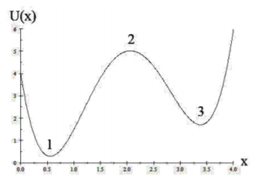
Figure 3.2.1:Stability for a one-dimensional potential U(x).
Figure 3.2.1 illustrates a conservative system that has three locations at which the restoring force is zero, that is, where the gradient of the potential is zero. Stable oscillations occur only around locations 1 and 3 whereas the system is unstable at the zero gradient location 2. Point 2 is called a separatrix in that an infinitesimal displacement of the particle from this separatrix will cause the particle to diverge towards either minimum 1 or 3 depending on which side of the separatrix the particle is displaced.
The requirements for stable oscillations about any point are that the potential energy must have the following properties.
Stability requirements
The potential has a stable position for which the restoring force is zero, i.e.
The potential must be positive and an even function of displacement . That is. where is even.
The requirement for the restoring force to be linear is that the restoring force for perturbation about a stable equilibrium at is of the form
The potential energy function for a linear oscillator has a pure parabolic shape about the minimum location, that is,
where is the location of the minimum.
Most oscillatory systems involve small amplitude oscillations about a stable minimum. For weak non-linear systems, where the amplitude of oscillation about the minimum is small, it is useful to make a Taylor expansion of the potential energy about the minimum. That is
By definition, at the minimum and thus Equation 3.3 can be written as
For small amplitude oscillations, the system is linear if the second-order term in Equation 3.2 is dominant.
The linearity for small amplitude oscillations greatly simplifies description of the oscillatory motion and complicated chaotic motion is avoided. Most physical systems are approximately linear for small amplitude oscillations, and thus the motion close to equilibrium approximates a linear harmonic oscillator.
3.3: Linearity and Superposition
An important aspect of linear systems is that the solutions obey the Principle of Superposition, that is, for the superposition of different oscillatory modes, the amplitudes add linearly. The linearly-damped linear oscillator is an example of a linear system in that it involves only linear operators, that is, it can be written in the operator form (appendix 19.6.2)
The quantity in the brackets on the left hand side is a linear operator that can be designated by where
An important feature of linear operators is that they obey the principle of superposition. This property results from the fact that linear operators are distributive, that is
Therefore if there are two solutions and for two different forcing functions and
then the addition of these two solutions, with arbitrary constants, also is a solution for linear operators.
In general then
The left hand bracket can be identified as the linear combination of solutions
while the driving force is a linear superposition of harmonic forces
Thus these linear combinations also satisfy the general linear equation
Applicability of the Principle of Superposition to a system provides a tremendous advantage for handling and solving the equations of motion of oscillatory systems.
3.4: Geometrical Representations of Dynamical Motion
The powerful pattern-recognition capabilities of the human brain, coupled with geometrical representations of the motion of dynamical systems, provide a sensitive probe of periodic motion. The geometry of the motion often can provide more insight into the dynamics than inspection of mathematical functions. A system with degrees of freedom is characterized by locations , velocities , and momenta , in addition to the time and instantaneous energy . Geometrical representations of the dynamical correlations are illustrated by the configuration space and phase space representations of these variables.
Configuration space 
A configuration space plot shows the correlated motion of two spatial coordinates and averaged over time. An example is the two-dimensional linear oscillator with two equations of motion and solutions
where . For unequal restoring force constants, the trajectory executes complicated Lissajous figures that depend on the angular frequencies and the phase factor . When the ratio of the angular frequencies along the two axes is rational, that is is a rational fraction, then the curve will repeat at regular intervals as shown in Figure 3.4.1, and this shape depends on the phase difference. Otherwise the trajectory gradually fills the whole rectangle.
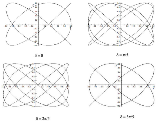
Figure 3.4.1:Configuration plots of where and at four different phase values . The curves are called Lissajous figures
State space, 
Visualization of a trajectory is enhanced by correlation of configuration and it’s corresponding velocity which specifies the direction of the motion. The state space representation[1] is especially valuable when discussing Lagrangian mechanics which is based on the Lagrangian .
The free undamped harmonic oscillator provides a simple application of state space. Consider a mass attached to a spring with linear spring constant for which the equation of motion is
By integration this gives
The first term in Equation 3.18 is the kinetic energy, the second term is the potential energy, and is the total energy which is conserved for this system. This equation can be expressed in terms of the state space coordinates as
This corresponds to the equation of an ellipse for a state-space plot of versus as shown in Figure 3.4.2-upper. The elliptical paths shown correspond to contours of constant total energy which is partitioned between kinetic and potential energy. For the coordinate axis shown, the motion of a representative point will be in a clockwise direction as the total oscillator energy is redistributed between potential to kinetic energy. The area of the ellipse is proportional to the total energy .
Phase space, 
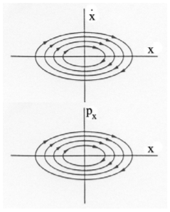
Figure 3.4.2:State space (upper), and phase space (lower) diagrams, for the linear harmonic oscillator.
Phase space, which was introduced by J.W. Gibbs for the field of statistical mechanics, provides a fundamental graphical representation in classical mechanics. The phase space coordinates are the conjugate coordinates and are fundamental to Hamiltonian mechanics which is based on the Hamiltonian . For a conservative system, only one phase-space curve passes through any point in phase space like the flow of an incompressible fluid. This makes phase space more useful than state space where many curves pass through any location. Lanczos [La49] defined an extended phase space using four-dimensional relativistic space-time as discussed in chapter 17.
Since for the non-relativistic, one-dimensional, linear oscillator, then Equation 3.19 can be rewritten in the form
This is the equation of an ellipse in the phase space diagram shown in Fig.3.4.2-lower which looks identical to Fig.3.4.2-upper since that the ordinate variable is multiplied by the constant . That is, the only difference is the phase-space coordinates replace the state-space coordinates . State space plots are used extensively in this chapter to describe oscillatory motion. Although phase space is more fundamental, both state space and phase space plots provide useful representations for characterizing and elucidating a wide variety of motion in classical mechanics. The following discussion of the undamped simple pendulum illustrates the general features of state space.
Plane pendulum
Consider a simple plane pendulum of mass attached to a string of length in a uniform gravitational field . There is only one generalized coordinate, . Since the moment of inertia of the simple plane-pendulum is then the kinetic energy is
and the potential energy relative to the bottom dead center is
Thus the total energy equals
where is a constant of motion. Note that the angular momentum is not a constant of motion since the angular acceleration explicitly depends on .
It is interesting to look at the solutions for the equation of motion for a plane pendulum on a state space diagram shown in Figure 3.4.3. The curves shown are equally-spaced contours of constant total energy. Note that the trajectories are ellipses only at very small angles where , the contours are non-elliptical for higher amplitude oscillations. When the energy is in the range the motion corresponds to oscillations of the pendulum about . The center of the ellipse is at which is a stable equilibrium point for the oscillation. However, when there is a phase change to rotational motion about the horizontal axis, that is, the pendulum swings around and over top dead center, i.e. it rotates continuously in one direction about the horizontal axis. The phase change occurs at . and is designated by the separatrix trajectory.
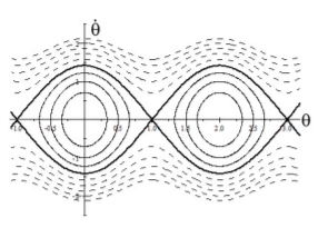
Figure 3.4.3:State space diagram for a plane pendulum. The \theta axis is in units of radians. Note that and correspond to the same physical point, that is the phase diagram should be rolled into a cylinder connected at .
Figure 3.4.3 shows two cycles for to better illustrate the cyclic nature of the phase diagram. The closed loops, shown as fine solid lines, correspond to pendulum oscillations about or for . The dashed lines show rolling motion for cases where the total energy . The broad solid line is the separatrix that separates the rolling and oscillatory motion. Note that at the separatrix the kinetic energy and are zero when the pendulum is at top dead center which occurs when . The point is an unstable equilibrium characterized by phase lines that are hyperbolic to this unstable equilibrium point. Note that and correspond to the same physical point, that is, the phase diagram is better presented on a cylindrical phase space representation since is a cyclic variable that cycles around the cylinder whereas oscillates equally about zero having both positive and negative values. The state-space diagram can be wrapped around a cylinder, then the unstable and stable equilibrium points will be at diametrically opposite locations on the surface of the cylinder at . For small oscillations about equilibrium, also called librations, the correlation between and is given by the clockwise closed loops wrapped on the cylindrical surface, whereas for energies the positive corresponds to counterclockwise rotations while the negative corresponds to clockwise rotations.
State-space diagrams will be used for describing oscillatory motion in chapters 3 and 4. Phase space is used in statistical mechanics in order to handle the equations of motion for ensembles of independent particles since momentum is more fundamental than velocity. Rather than try to account separately for the motion of each particle for an ensemble, it is best to specify the region of phase space containing the ensemble. If the number of particles is conserved, then every point in the initial phase space must transform to corresponding points in the final phase space. This will be discussed in chapters 8.3 and 15.2.7.
3.5: Linearly-damped Free Linear Oscillator
General solution
All simple harmonic oscillations are damped to some degree due to energy dissipation via friction, viscous forces, or electrical resistance etc. The motion of damped systems is not conservative since energy is dissipated as heat. As was discussed in chapter 2 the damping force can be expressed as
where the velocity dependent function can be complicated. Fortunately there is a very large class of problems in electricity and magnetism, classical mechanics, molecular, atomic, and nuclear physics, where the damping force depends linearly on velocity which greatly simplifies solution of the equations of motion. Therefore this chapter will discuss linear damping.
Consider the free simple harmonic oscillator, that is, assuming no oscillatory forcing function, with a linear damping term where the parameter is the damping factor. Then the equation of motion is
This can be rewritten as
where the damping parameter
and the characteristic angular frequency
The general solution to the linearly-damped free oscillator is obtained by inserting the complex trial solution . Then
This implies that
The solution is
The two solutions are complex conjugates and thus the solutions of the damped free oscillator are
This can be written as
where
Underdamped motion 
When then the square root is real so the solution can be written taking the real part of which gives that Equation 3.33 equals
Where and are adjustable constants fit to the initial conditions. Therefore the velocity is given by
This is the damped sinusoidal oscillation illustrated in Figure 3.5.1-upper. The solution has the following characteristics:
The oscillation amplitude decreases exponentially with a time constant .
There is a small reduction in the frequency of the oscillation due to the damping leading to
![The amplitude-time dependence and state-space diagrams for the free linearly-damped harmonic oscillator. The upper row shows the underdamped system for the case with damping \Gamma = \frac{\omega_0}{5\pi}. The lower row shows the overdamped ( \frac{\Gamma}{ 2} > \omega_0) [solid line] and critica…](/variationalPrinciples/build/lt-21115-3-789f28b48ef5661f6ad194fa759cfecb.5.1.png)
Figure 3.5.1:The amplitude-time dependence and state-space diagrams for the free linearly-damped harmonic oscillator. The upper row shows the underdamped system for the case with damping . The lower row shows the overdamped [solid line] and critically damped [dashed line] in both cases assuming that initially the system is at rest.
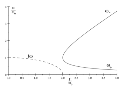
Figure 3.5.2:Real and imaginary solutions of the damped harmonic oscillator. A phase transition occurs at . For (dashed) the two solutions are complex conjugates and imaginary. For , (solid), there are two real solutions and with widely different decay constants where dominates the decay at long times.
Overdamped case 
In this case the square root of is imaginary and can be expressed as . Therefore the solution is obtained more naturally by using a real trial solution in Equation 3.33 which leads to two roots
Thus the exponentially damped decay has two time constants and .
The time constant thus the first term in the bracket decays in a shorter time than the second term . As illustrated in Figure 3.5.2 the decay rate, which is imaginary when underdamped, i.e. bifurcates into two real values for overdamped, i.e. . At large times the dominant term when overdamped is for which has the smallest decay rate, that is, the longest decay constant . There is no oscillatory motion for the overdamped case, it slowly moves monotonically to zero as shown in fig 3.5 lower. The amplitude decays away with a time constant that is longer than .
Critically damped 
This is the limiting case where For this case the solution is of the form
This motion also is non-sinusoidal and evolves monotonically to zero. As shown in Figure 3.5.1 the critically-damped solution goes to zero with the shortest time constant, that is, largest . Thus analog electric meters are built almost critically damped so the needle moves to the new equilibrium value in the shortest time without oscillation.
It is useful to graphically represent the motion of the damped linear oscillator on either a state space diagram or phase space diagram as discussed in chapter 3.4. The state space plots for the undamped, overdamped, and critically-damped solutions of the damped harmonic oscillator are shown in Figure 3.5.1. For underdamped motion the state space diagram spirals inwards to the origin in contrast to critical or overdamped motion where the state and phase space diagrams move monotonically to zero.
Energy dissipation
The instantaneous energy is the sum of the instantaneous kinetic and potential energies
where and are given by the solution of the equation of motion. Consider the total energy of the underdamped system
where . The average total energy is given by substitution for and and taking the average over one cycle. Since
Then the velocity is given by
Inserting equations 3.41 and 3.42 into 3.40 gives a small amplitude oscillation about an exponential decay for the energy . Averaging over one cycle and using the fact that , and , gives the time-averaged total energy as
which can be written as
Note that the energy of the linearly damped free oscillator decays away exponentially with a time constant . That is, the intensity has a time constant that is half the time constant for the decay of the amplitude of the transient response. Note that the average kinetic and potential energies are identical, as implied by the Virial theorem, and both decay away with the same time constant. This relation between the mean life for decay of the damped harmonic oscillator and the damping width term occurs frequently in physics.
The damping of an oscillator usually is characterized by a single parameter called the Quality Factor where
The energy loss per radian is given by
where the numerator is the frequency of the free damped linear oscillator.
Thus the Quality factor equals
The larger the factor, the less damped is the system, and the greater is the number of cycles of the oscillation in the damped wave train. Chapter 3.11.3 shows that the longer the wave train, that is the higher is the factor, the narrower is the frequency distribution around the central value. The Mössbauer effect in nuclear physics provides a remarkably long wave train that can be used to make high precision measurements. The high- precision of the LIGO laser interferometer was used in the recent successful search for gravity waves.
| Oscillating system | Typical Q factors |
|---|---|
| Earth, for earthquake wave | 250-1400 |
| Piano string | 3000 |
| Crystal in digital watch | 104 |
| Microwave cavity | 104 |
| Excited atom | 107 |
| Neutron star | 1012 |
| LIGO laser | 1013 |
| Mössbauer effect in nucleus | 1014 |
3.6: Sinusoidally-driven, linearly-damped, linear oscillator
The linearly-damped linear oscillator, driven by a harmonic driving force, is of considerable importance to all branches of science and engineering. The equation of motion can be written as
where is the driving force. For mathematical simplicity the driving force is chosen to be a sinusoidal harmonic force. The solution of this second-order differential equation comprises two components, the complementary solution (transient response), and the particular solution (steady-state response).
Transient response of a driven oscillator
The transient response of a driven oscillator is given by the complementary solution of the above second-order differential equation
which is identical to the solution of the free linearly-damped harmonic oscillator. As discussed in section 3.5 the solution of the linearly-damped free oscillator is given by the real part of the complex variable where
and
Underdamped motion :
When , then the square root is real so the transient solution can be written taking the real part of which gives
The solution has the following characteristics:
a) The amplitude of the transient solution decreases exponentially with a time constant while the energy decreases with a time constant of .
b) There is a small downward frequency shift in that .
Overdamped case :
In this case the square root is imaginary, which can be expressed as which is real and the solution is just an exponentially damped one
There is no oscillatory motion for the overdamped case, it slowly moves monotonically to zero. The total energy decays away with two time constants greater than .
Critically damped :
For this case, as mentioned for the damped free oscillator, the solution is of the form
The critically-damped system decays away the quickest.
Steady state response of a driven oscillator
The particular solution of the differential equation gives the important steady state response, to the forcing function. Consider that the forcing term is a single frequency sinusoidal oscillation.
Thus the particular solution is the real part of the complex variable which is a solution of
A trial solution is
This leads to the relation
Multiplying the numerator and denominator by the factor gives
The steady state solution thus is given by the real part of , that is
This can be expressed in terms of a phase defined as
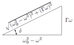
Figure 3.6.1:Phase between driving force and resultant motion.
As shown in Figure 3.6.1 the hypotenuse of the triangle equals . Thus
and
The phase represents the phase difference between the driving force and the resultant motion. For a fixed the phase when , and increases to when . For the phase as .
The steady state solution can be re-expressed in terms of the phase shift as
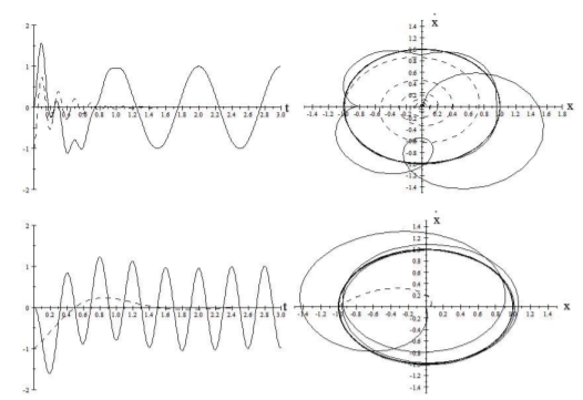
Figure 3.6.2:Amplitude versus time, and state space plots of the transient solution (dashed) and total solution (solid) for two cases. The upper row shows the case where the driving frequency while the lower row shows the same for the case where the driving frequency .
Complete solution of the driven oscillator
To summarize, the total solution of the sinusoidally forced linearly-damped harmonic oscillator is the sum of the transient and steady-state solutions of the equations of motion.
This for the underdamped case, the transient solution is the complementary solution
where . The steady-state solution is given by the particular solution
Note that the frequency of the transient solution is which in general differs from the driving frequency . The phase shift for the transient component is set by the initial conditions. The transient response leads to a more complicated motion immediately after the driving function is switched on. Figure 3.6.2 illustrates the amplitude time dependence and state space diagram for the transient component, and the total response, when the driving frequency is either or . Note that the modulation of the steady-state response by the transient response is unimportant once the transient response has damped out leading to a constant elliptical state space trajectory. For cases where the initial conditions are then the transient solution has a relative phase difference radians at and relative amplitudes such that the transient and steady-state solutions cancel at .
The characteristic sounds of different types of musical instruments depend very much on the admixture of transient solutions plus the number and mixture of oscillatory active modes. Percussive instruments, such as the piano, have a large transient component. The mixture of transient and steady-state solutions for forced oscillations occurs frequently in studies of RLC networks in electrical circuit analysis.
Resonance
The discussion so far has discussed the role of the transient and steady-state solutions of the driven damped harmonic oscillator which occurs frequently is science, and engineering. Another important aspect is resonance that occurs when the driving frequency approaches the natural frequency of the damped system. Consider the case where the time is sufficient for the transient solution to have decayed to zero.
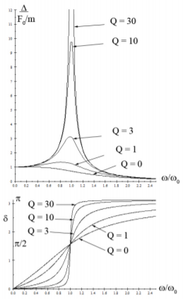
Figure 3.6.3:Resonance behavior for the linearly-damped, harmonically driven, linear oscillator.
Figure 3.6.3 shows the amplitude and phase for the steady-state response as goes through a resonance as the driving frequency is changed. The steady-states solution of the driven oscillator follows the driving force when in that the phase difference is zero and the amplitude is just . The response of the system peaks at resonance, while for the harmonic system is unable to follow the more rapidly oscillating driving force and thus the phase of the induced oscillation is out of phase with the driving force and the amplitude of the oscillation tends to zero.
Note that the resonance frequency for a driven damped oscillator, differs from that for the undriven damped oscillator, and differs from that for the undamped oscillator. The natural frequency for an undamped harmonic oscillator is given by
The transient solution is the same as damped free oscillations of a damped oscillator and has a frequency of the system given by
That is, damping slightly reduces the frequency.
For the driven oscillator the maximum value of the steady-state amplitude response is obtained by taking the maximum of the function , that is when . This occurs at the resonance angular frequency where
No resonance occurs if since then is imaginary and the amplitude decreases monotonically with increasing . Note that the above three frequencies are identical if but they differ when with .
For the driven oscillator it is customary to define the quality factor as
When then one has a narrow high resonance peak. As the damping increases the quality factor decreases leading to a wider and lower peak. The resonance disappears when .
Energy absorption
Discussion of energy stored in resonant systems is best described using the steady state solution which is dominant after the transient solution has decayed to zero. Then
This can be rewritten as
where the elastic amplitude
while the absorptive amplitude
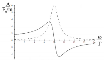
Figure 3.6.4:Elastic (solid) and absorptive (dashed) amplitudes of the steady-state solution for .
Figure 3.6.4 shows the behavior of the absorptive and elastic amplitudes as a function of angular frequency . The absorptive amplitude is significant only near resonance whereas the elastic amplitude goes to zero at resonance. Note that the full width at half maximum of the absorptive amplitude peak equals .
The work done by the force on the oscillator is
Thus the absorbed power is given by
The steady state response gives a velocity
Thus the steady-state instantaneous power input is
The absorptive term steadily absorbs energy while the elastic term oscillates as energy is alternately absorbed or emitted. The time average over one cycle is given by
where and are the time average over one cycle. The time averages over one complete cycle for the first term in the bracket is
while for the second term
Thus the time average power input is given by only the absorptive term
This shape of the power curve is a classic Lorentzian shape. Note that the maximum of the average kinetic energy occurs at which is different from the peak of the amplitude which occurs at . The potential energy is proportional to the amplitude squared, i.e. which occurs at the same angular frequency as the amplitude, that is, . The kinetic and potential energies resonate at different angular frequencies as a result of the fact that the driven damped oscillator is not conservative because energy is continually exchanged between the oscillator and the driving force system in addition to the energy dissipation due to the damping.
When , then the power equation simplifies since
Therefore
This is called the Lorentzian or Breit-Wigner shape. The half power points are at a frequency difference from resonance of where
Thus thefull width at half maximum of the Lorentzian curve equals . Note that the Lorentzian has a narrower peak but much wider tail relative to a Gaussian shape. At the peak of the absorbed power, the absorptive amplitude can be written as
That is, the peak amplitude increases with increase in . This explains the classic comedy scene where the soprano shatters the crystal glass because the highest quality crystal glass has a high which leads to a large amplitude oscillation when she sings on resonance.
The mean lifetime of the free linearly-damped harmonic oscillator, that is, the time for the energy of free oscillations to decay to was shown to be related to the damping coefficient by
Therefore we have the classical uncertainty principle for the linearly-damped harmonic oscillator that the measured full-width at half maximum of the energy resonance curve for forced oscillation and the mean life for decay of the energy of a free linearly-damped oscillator are related by
This relation is correct only for a linearly-damped harmonic system. Comparable relations between the lifetime and damping width exist for different forms of damping.
One can demonstrate the above line width and decay time relationship using an acoustically driven electric guitar string. It also occurs for the width of the electromagnetic radiation and the lifetime for decay of atomic or nuclear electromagnetic decay. This classical uncertainty principle is exactly the same as the one encountered in quantum physics due to wave-particle duality. In nuclear physics it is difficult to measure the lifetime of states when . For shorter lifetimes the value of can be determined from the shape of the resonance curve which can be measured directly when the damping is large.
3.7: Wave equation
Wave motion is a ubiquitous feature in nature. Mechanical wave motion is manifest by transverse waves on fluid surfaces, longitudinal and transverse seismic waves traveling through the Earth, and vibrations of mechanical structures such as suspended cables. Acoustical wave motion occurs on the stretched strings of the violin, as well as the cavities of wind instruments. Electromagnetic wave motion includes wavelengths ranging from radiowaves, to -rays. Matter waves are a prominent feature of quantum physics. All these manifestations of waves exhibit the same general features of wave motion.
Wave motion occurs for deformable bodies where elastic forces acting between the nearest-neighbor atoms of the body exert time-dependent forces on one another. Chapter 14 will introduce the collective modes of motion, called the normal modes, of coupled, many-body, linear oscillators which act as independent modes of motion. However, it is useful to introduce wavemotion at this juncture because the equations of wave motion are simple, and wave motion features prominently in several chapters of this book.
Consider a traveling wave in one dimension for a linear system. If the wave is moving, then the wave function describing the shape of the wave, is a function of both and . The instantaneous amplitude of the wave could correspond to the transverse displacement of a wave on a string, the longitudinal amplitude of a wave on a spring, the pressure of a longitudinal sound wave, the transverse electric or magnetic fields in an electromagnetic wave, a matter wave, etc. If the wave train maintains its shape as it moves, then one can describe the wave train by the function where the coordinate is measured relative to the shape of the wave, that is, it could correspond to the phase of a crest of the wave. Consider that corresponds to a constant phase, e.g. the peak of the traveling pulse, then assuming that the wave travels at a phase velocity in the direction and the peak is at for , then it is at at time . That is, a point with phase fixed with respect to the waveform shape of the wave profile moves in the direction for and in direction for .
General wave motion can be described by solutions of a wave equation. The wave equation can be written in terms of the spatial and temporal derivatives of the wave function . Consider the first partial derivatives of = .
and
Factoring out for the first derivatives gives
The sign in this equation depends on the sign of the wave velocity making it not a generally useful formula.
Consider the second derivatives
and
Factoring out gives
This wave equation in one dimension for a linear system is independent of the sign of the velocity. There are an infinite number of possible shapes of waves both traveling and standing in one dimension, all of these must satisfy this one-dimensional wave equation. The converse is that any function that satisfies this one dimensional wave equation must be a wave in this one dimension.
The Wave Equation in three dimensions is
There are an infinite number of possible solutions to this wave equation, any one of which corresponds to a wave motion with velocity .
The Wave Equation is applicable to all manifestations of wave motion, both transverse and longitudinal, for linear systems. That is, it applies to waves on a string, water waves, seismic waves, sound waves, electromagnetic waves, matter waves, etc. If it can be shown that a wave equation can be derived for any system, discrete or continuous, then this is equivalent to proving the existence of waves of any waveform, frequency, or wavelength traveling with the phase velocity given by the wave equation.[Cra65]
3.8: Traveling and standing wave solutions of the wave equation
The wave equation can have both traveling and standing-wave solutions. Consider a one-dimensional traveling wave with velocity having a specific wavenumber . Then the traveling wave is best written in terms of the phase of the wave as
where the wave number , with being the wave length, and angular frequency . This particular solution satisfies the wave equation and corresponds to a traveling wave with phase velocity in the positive or negative direction depending on whether the sign is negative or positive. Assuming that the superposition principle applies, then the superposition of these two particular solutions of the wave equation can be written as
Thus the superposition of two identical single wavelength traveling waves propagating in opposite directions can correspond to a standing wave solution. Note that a standing wave is identical to a stationary normal mode of the system discussed in chapter 14. This transformation between standing and traveling waves can be reversed, that is, the superposition of two standing waves, i.e. normal modes, can lead to a traveling wave solution of the wave equation. Discussion of waveforms is simplified when using either of the following two limits.
The time dependence of the waveform at a given location which can be expressed using a Fourier decomposition, appendix 19.9.2, of the time dependence as a function of angular frequency .
The spatial dependence of the waveform at a given instant which can be expressed using a Fourier decomposition of the spatial dependence as a function of wavenumber
The above is applicable both to discrete, or continuous linear oscillator systems, e.g. waves on a string. In summary, stationary normal modes of a system are obtained by a superposition of traveling waves traveling in opposite directions, or equivalently, traveling waves can result from a superposition of stationary normal modes.
3.9: Waveform Analysis
Harmonic decomposition
As described in appendix 19.9, when superposition applies, then a Fourier series decomposition of the form 3.101 can be made of any periodic function where
or the more general Fourier Transform can be made for an aperiodic function where
Any linear system that is subject to the forcing function has an output that can be expressed as a linear superposition of the solutions of the individual harmonic components of the forcing function. Fourier analysis of periodic waveforms in terms of harmonic trigonometric functions plays a key role in describing oscillatory motion in classical mechanics and signal processing for linear systems. Fourier’s theorem states that any arbitrary forcing function can be decomposed into a sum of harmonic terms. As a consequence two equivalent representations can be used to describe signals and waves; the first is in the time domain which describes the time dependence of the signal. The second is in the frequency domain which describes the frequency decomposition of the signal. Fourier analysis relates these equivalent representations.
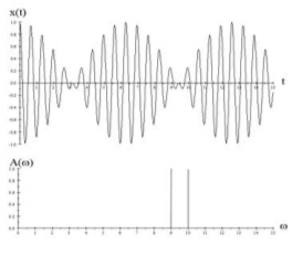
Figure 3.9.1:The time and frequency representations of a system exhibiting beats.
For example, the superposition of two equal intensity harmonic oscillators in the time domain is given by
The free linearly-damped linear oscillator
The response of the free, linearly-damped, linear oscillator is one of the most frequently encountered waveforms in science and thus it is useful to investigate the Fourier transform of this waveform. The damped waveform for the underdamped case, shown in figure (3.5.1) is given by equation (3.5.12), that is
where and where is the angular frequency of the underdamped system. The Fourier transform is given by
which is complex and has the famous Lorentz form.
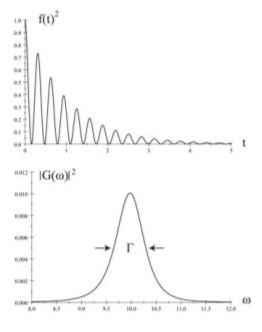
Figure 3.9.2:The intensity and Fourier transform of the free linearly-underdamped harmonic oscillator with and damping .
The intensity of the wave gives
Note that since the average over of , then the average over the term gives the intensity which has a mean lifetime for the decay of . The distribution has the classic Lorentzian shape, shown in Figure 3.9.2, which has a full width at half-maximum, FWHM, equal to . Note that is complex and thus one also can determine the phase shift which is given by the ratio of the imaginary to real parts of Equation 3.105, i.e. .
The mean lifetime of the exponential decay of the intensity can be determined either by measuring from the time dependence, or measuring the FWHM of the Fourier transform . In nuclear and atomic physics excited levels decay by photon emission with the wave form of the free linearly-damped, linear oscillator. Typically the mean lifetime usually can be measured when whereas for shorter lifetimes the radiation width becomes sufficiently large to be measured. Thus the two experimental approaches are complementary.
Damped linear oscillator subject to an arbitrary periodic force
Fourier’s theorem states that any arbitrary forcing function can be decomposed into a sum of harmonic terms. Consider the response of a damped linear oscillator to an arbitrary periodic force.
For each harmonic term the response of a linearly-damped linear oscillator to the forcing function is given by equation (3.6.18-3.6.20) to be
The amplitude is obtained by substituting into Equation 3.110 the derived values from the Fourier analysis.
3.10: Signal Processing
It has been shown that the response of the linearly-damped linear oscillator, subject to any arbitrary periodic force, can be calculated using a frequency decomposition, (Fourier analysis), of the force, appendix 19.9. The response can equally well can be calculated using a time-ordered discrete-time sampling of the pulse shape; that is, the Green’s function approach, appendix 19.9. The linearly-damped, linear oscillator is the simplest example of a linear system that exhibits both resonance and frequency-dependent response. Typical physical linear systems exhibit far more complicated response functions with multiple resonances and corresponding frequency response. For example, an automobile suspension system involves four wheels and associated springs plus dampers allowing the car to rock sideways, or forward and backward, in addition to the updown motion, when subject to the forces produced by a rough road. Similarly a suspension bridge or aircraft wing can twist as well as bend due to air turbulence, or a building can undergo complicated oscillations due to seismic waves. An acoustic system exhibits similar complexity. Signal analysis and signal processing is of pivotal importance to elucidating the response of complicated linear systems to complicated periodic forcing functions. This is used extensively in engineering, acoustics, and science.
The response of a low-pass filter, such as an R-C circuit or a coaxial cable, to a input square wave, shown in Figure 3.10.1, provides a simple example of the relative advantages of using the complementary Fourier analysis in the frequency domain, or the Green’s discrete-function analysis in the time domain. The response of a repetitive square-wave input signal is shown in the time domain and the Fourier transform to the frequency domain. The middle curves show the time dependence for the response of the low-pass filter to an impulse and the Fourier transform . The output of the low-pass filter can be calculated by folding the input square wave and impulse time dependence in the time domain as shown on the left or by folding of their Fourier transforms shown on the right. Working in the frequency domain the response of linear mechanical systems, such as an automobile suspension or a musical instrument, as well as linear electronic signal processing systems such as amplifiers, loudspeakers and microphones, can be treated as black boxes having a certain transfer function describing the gain and phase shift versus frequency. That is, the output wave frequency decomposition is
Working in the time domain, the low-pass system has an impulse response , which is the Fourier transform of the transfer function . In the time domain
This is shown schematically in Figure 3.10.1. The Fourier transformation connects the three quantities in the time domain with the corresponding three in the frequency domain. For example, the impulse response of the low-pass filter has a fall time of which is related by a Fourier transform to the width of the transfer function. Thus the time and frequency domain approaches are closely related and give the same result for the output signal for the low-pass filter to the applied square-wave input signal. The result is that the higher-frequency components are attenuated leading to slow rise and fall times in the time domain.
Analog signal processing and Fourier analysis were the primary tools to analyze and process all forms of periodic motion during the 20 century. For example, musical instruments, mechanical systems, electronic circuits, all employed resonant systems to enhance the desired frequencies and suppress the undesirable frequencies and the signals were observed using analog oscilloscopes. The remarkable development of computing has enabled use of digital signal processing leading to a revolution in signal processing that has had a profound impact on both science and engineering. For example, the digital oscilloscope, which can sample at frequencies above 109 has replaced the analog oscilloscope because it allows sophisticated analysis of each individual signal that was not possible using analog signal processing. For example, the analog approach in nuclear physics involved tiny analog electric signals, produced by many individual radiation detectors, that were transmitted hundreds of meters via carefully shielded and expensive coaxial cables to the data room where the signals were amplified and signal processed using analog filters to maximize the signal to noise in order to separate the signal from the background noise. Stray electromagnetic radiation picked up via the cables significantly degraded the signals. The performance and limitations of the analog electronics severely restricted the pulse processing capabilities. Digital signal processing has rapidly replaced analog signal processing. Analog to digital detector circuits are built directly into the electronics for each individual detector so that only digital information needs to be transmitted from each detector to the analysis computers. Computer processing provides unlimited and flexible processing capabilities for the digital signals greatly enhancing the response and sensitivity of our detector systems. Common examples of digital signal processing are digital CD and DVD disks.
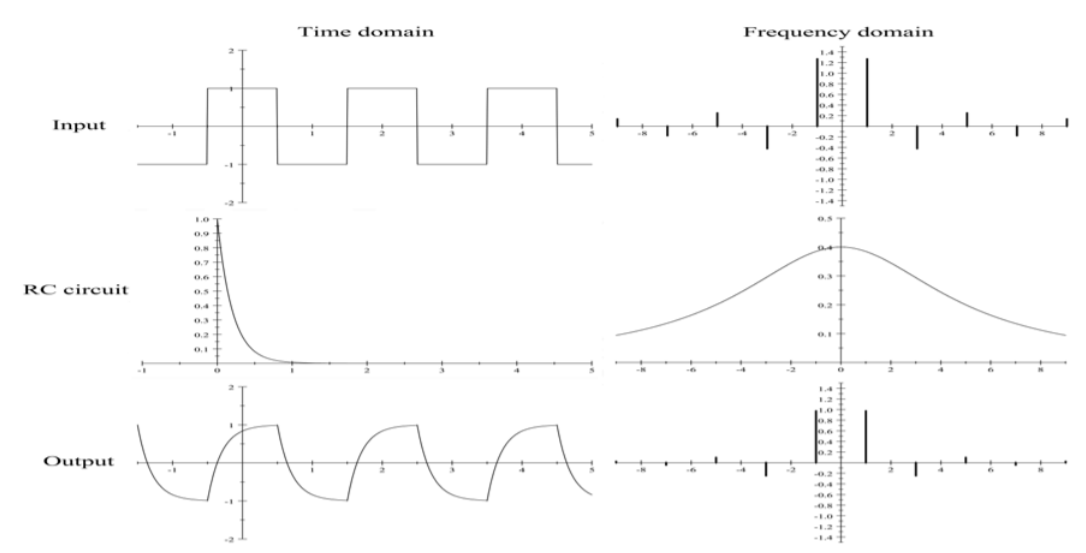
Figure 3.10.1:Response of an RC electrical circuit to an input square wave. The upper row shows the time and the exponential-form frequency representations of the square-wave input signal. The middle row gives the impulse response, and corresponding transfer function for the RC circuit. The bottom row shows the corresponding output properties in both the time and frequency domains
3.11: Wave Propagation
Wave motion typically involves a packet of waves encompassing a finite number of wave cycles. Information in a wave only can be transmitted by starting, stopping, or modulating the amplitude of a wave train, which is equivalent to forming a wave packet. For example, a musician will play a note for a finite time, and this wave train propagates out as a wave packet of finite length. You have no information as to the frequency and amplitude of the sound prior to the wave packet reaching you, or after the wave packet has passed you. The velocity of the wavelets contained within the wave packet is called the phase velocity. For a dispersive system the phase velocity of the wavelets contained within the wave packet is frequency dependent and the shape of the wave packet travels at the group velocity which usually differs from the phase velocity. If the shape of the wave packet is time dependent, then neither the phase velocity, which is the velocity of the wavelets, nor the group velocity, which is the velocity of an instantaneous point fixed to the shape of the wave packet envelope, represent the actual velocity of the overall wavepacket.
A third wavepacket velocity, the signal velocity, is defined to be the velocity of the leading edge of the energy distribution, and corresponding information content, of the wave packet. For most linear systems the shape of the wave packet is not time dependent and then the group and signal velocities are identical. However, the group and signal velocities can be very different for non-linear systems as discussed in chapter 4.7. Note that even when the phase velocity of the waves within the wave packet travels faster than the group velocity of the shape, or the signal velocity of the energy content of the envelope of the wave packet, the information contained in a wave packet is only manifest when the wave packet envelope reaches the detector and this energy and information travel at the signal velocity.
The modern ideas of wave propagation, including Hamilton’s concept of group velocity, were developed by Lord Rayleigh when applied to the theory of sound[Ray1887]. The concept of phase, group, and signal velocities played a major role in discussion of electromagnetic waves as well as de Broglie’s development of the concept of wave-particle duality and the development of wave mechanics by Schrödinger.
Phase, group, and signal velocities of wave packets
The concepts of wave packets, as well as their phase, group, and signal velocities, are of considerable importance for propagation of information and other manifestations of wave motion in science and engineering which warrants further discussion at this juncture.
Consider a particular , component of a one-dimensional wave,
The argument of the exponential is called the phase of the wave where
If we move along the axis at a velocity such that the phase is constant then we perceive a stationary wave. The velocity of this wave is called the phase velocity. To ensure constant phase we require that is constant or, assuming real and
Therefore the phase velocity is defined to be
The velocity we have used so far is just the phase velocity of the individual wavelets at the carrier frequency. If or are complex then one must take the real parts to ensure that the velocity is real.
If the phase velocity of a wave is dependent on the wavelength, that is, , then the system is said to be dispersive in that the wave is dispersed according the wavelength. The simplest illustration of dispersion is the refraction of light in glass prism which leads to dispersion of the light into the spectrum of wavelengths. Dispersion leads to development of wave packets that travel at group and signal velocities that usually differ from the phase velocity. To illustrate this consider two equal amplitude traveling waves having slightly different wave number and angular frequency . Superposition of these waves gives
This corresponds to a wave with the average carrier frequency modulated by the cosine term which has a wavenumber of and angular frequency , that is, this is the usual example of beats. The cosine term modulates the average wave producing wave packets as shown in figure (3.9.1). The velocity of these wave packets is called the group velocity given by requiring that the phase of the modulating term is constant, that is
Thus the group velocity is given by
If dispersion is present then the group velocity does not equal the phase velocity .
Expanding the above example to superposition of waves gives
In the event that and the frequencies are continuously distributed, then the summation is replaced by an integral
where the factor represents the distribution amplitudes of the component waves, that is the spectral decomposition of the wave. This is the usual Fourier decomposition of the spatial distribution of the wave.
Consider an extension of the linear superposition of two waves to a well defined wave packet where the amplitude is nonzero only for a small range of wavenumbers .
This functional shape is called a wave packet which only has meaning if . The angular frequency can be expressed by making a Taylor expansion around
For a linear system the phase then reduces to
The summation of terms in the exponent given by 3.125 leads to the amplitude 3.123 having the form of a product where the integral becomes
The integral term modulates the first term.
The group velocity is defined to be that for which the phase of the exponential term in the integral is constant. Thus
Since then
For non-dispersive systems the phase velocity is independent of the wave number or angular frequency and thus . The case discussed earlier, equation (3.9.3), for beating of two waves gives the same relation in the limit that and are infinitesimal.
The group velocity of a wave packet is of physical significance for dispersive media where . Every wave train has a finite extent and thus we usually observe the motion of a group of waves rather than the wavelets moving within the wave packet. In general, for non-linear dispersive systems the derivative can be either positive or negative and thus in principle the group velocity can either be greater than, or less than, the phase velocity. Moreover, if the group velocity is frequency dependent, that is, when group velocity dispersion occurs, then the overall shape of the wave packet is time dependent and thus the speed of a specific relative location defined by the shape of the envelope of the wave packet does not represent the signal velocity of the wave packet. Brillouin showed that the distribution of the energy, and corresponding information content, in any wave packet travels at the signal velocity which can be different from the group velocity if the shape of the envelope of the wave packet is time dependent. For electromagnetic waves one has the possibility that the group velocity . In 1914 Brillouin[Bri14][Bri60] showed that the signal velocity of electromagnetic waves, defined by the leading edge of the time-dependent envelope of the wave packet, never exceeds even though the group velocity corresponding to the velocity of the instantaneous shape of the wave packet may exceed . Thus, there is no violation of Einstein’s fundamental principle of relativity that the velocity of an electromagnetic wave cannot exceed .
Fourier transform of wave packets
The relation between the time distribution and the corresponding frequency distribution, or equivalently, the spatial distribution and the corresponding wave-number distribution, are of considerable importance in discussion of wave packets and signal processing. It directly relates to the uncertainty principle that is a characteristic of all forms of wave motion. The relation between the time and corresponding frequency distribution is given via the Fourier transform discussed in appendix 19.9. The following are two examples of the Fourier transforms of typical but rather different wavepacket shapes that are encountered frequently in science and engineering.
Wave-packet Uncertainty Principle
The Uncertainty Principle states that for all types of wave motion there is a minimum product of the uncertainty in the width of a wave packet and the distribution width of the frequency decomposition of the wave packet. This was illustrated by the Fourier transforms of wave packets discussed above where it was shown the product of the widths is minimized for a Gaussian-shaped wave packet. The Uncertainty Principle implies that to make a precise measurement of the frequency of a sinusoidal wave requires that the wave packet be infinitely long. If the length of the wave packet is reduced then the frequency distribution broadens. Then the crucial aspect needed for this discussion, is that, for the amplitudes of any wavepacket, the standard deviations characterizing the width of the spectral distribution in the angular frequency domain, , and the width in time are related:
This product of the standard deviations equals unity only for the special case of Gaussian-shaped spectral distributions, and is greater than unity for all other shaped spectral distributions.
The intensity of the wave is the square of the amplitude leading to standard deviation widths for a Gaussian distribution where , that is, . Thus the standard deviations for the spectral distribution and width of the intensity of the wavepacket are related by:
This states that the uncertainties with which you can simultaneously measure the time and frequency for the intensity of a given wavepacket are related. If you try to measure the frequency within a short time interval then the uncertainty in the frequency measurement . Accurate measurement of the frequency requires measurement times that encompass many cycles of oscillation, that is, a long wavepacket.
Exactly the same relations exist between the spectral distribution as a function of wavenumber and the spatial dependence of a wave which are conjugate representations. Thus the spectral distribution plotted versus is directly related to the amplitude as a function of position ; the spectral distribution versus is related to the amplitude as a function of ; and the spectral distribution is related to the spatial dependence on . Following the same arguments discussed above, the standard deviation, characterizing the width of the spectral intensity distribution of , and the standard deviation , characterizing the spatial width of the wave packet intensity as a function of , are related by the Uncertainty Principle for position-wavenumber. Thus in summary the uncertainty principle for the intensity of wave motion is,
This applies to all forms of wave motion, be they, sound waves, water waves, electromagnetic waves, or matter waves.
As discussed in chapter 18, the transition to quantum mechanics involves relating the matter-wave properties to the energy and momentum of the corresponding particle. That is, in the case of matter waves, multiplying both sides of Equation 3.128 by and using the de Broglie relations gives that the particle energy is related to the angular frequency by and the particle momentum is related to the wavenumber, that is . These lead to the Heisenberg Uncertainty Principle:
This uncertainty principle applies equally to the wavefunction of the electron in the hydrogen atom, proton in a nucleus, as well as to a wavepacket describing a particle wave moving along some trajectory. Thus, this implies that, for a particle of given momentum, the wavefunction is spread out spatially. Planck’s constant is extremely small compared with energies and times encountered in normal life, and thus the effects due to the Uncertainty Principle are not manifest for macroscopic dimensions.
Confinement of a particle, of mass , within of a fixed location implies that there is a corresponding uncertainty in the momentum
Now the variance in momentum is given by the difference in the average of the square , and the square of the average of . That is
Assuming a fixed average location implies that , then
Since the kinetic energy is given by:
This zero-point energy is the minimum kinetic energy that a particle of mass can have if confined within a distance . This zero-point energy is a consequence of wave-particle duality and the uncertainty between the size and wavenumber for any wave packet. It is a quantal effect in that the classical limit has for which the zero-point energy .
Inserting numbers for the zero-point energy gives that an electron confined to the radius of the atom, that is , has a zero-point kinetic energy of . Confining this electron to , the size of a nucleus, gives a zero-point energy of . Confining a proton to the size of the nucleus gives a zero-point energy of 0.5 . These values are typical of the level spacing observed in atomic and nuclear physics. If was a large number, then a billiard ball confined to a billiard table would be a blur as it oscillated with the minimum zero-point kinetic energy. The smaller the spatial region that the ball was confined, the larger would be its zero-point energy and momentum causing it to rattle back and forth between the boundaries of the confined region. Life would be dramatically different if was a large number.
In summary, Heisenberg’s Uncertainty Principle is a well-known and crucially important aspect of quantum physics. What is less well known, is that the Uncertainty Principle exists for all forms of wave motion, that is, it is not restricted to matter waves. The following three examples illustrate application of the Uncertainty Principle to acoustics, the nuclear Mössbauer effect, and quantum mechanics.
3.E: Linear Oscillators (Exercises)
Consider a simple harmonic oscillator consisting of a mass attached to a spring of spring constant . For this oscillator .
Find an expression for .
Eliminate between and to arrive at one equation similar to that for an ellipse.
Rewrite the equation in part (b) in terms of , and the total energy .
Give a rough sketch of the phase space diagram ( versus ) for this oscillator. Also, on the same set of axes, sketch the phase space diagram for a similar oscillator with a total energy that is larger than the first oscillator.
What direction are the paths that you have sketched? Explain your answer.
Would different trajectories for the same oscillator ever cross paths? Why or why not?
Consider a damped, driven oscillator consisting of a mass attached to a spring of spring constant .
What is the equation of motion for this system?
Solve the equation in part (a). The solution consists of two parts, the complementary solution and the particular solution. When might it be possible to safely neglect one part of the solution?
What is the difference between amplitude resonance and kinetic energy resonance?
How might phase space diagrams look for this type of oscillator? What variables would affect the diagram?
A particle of mass is subject to the following force
where is a constant.
Determine the points when the particle is in equilibrium.
Which of these points is stable and which are unstable?
Is the motion bounded or unbounded?
A very long cylindrical shell has a mass density that depends upon the radial distance such that , where is a constant. The inner radius of the shell is and the outer radius is .
Determine the direction and the magnitude of the gravitational field for all regions of space.
If the gravitational potential is zero at the origin, what is the difference between the gravitational potential at and ?
A mass is constrained to move along one dimension. Two identical springs are attached to the mass, one on each side, and each spring is in turn attached to a wall. Both springs have the same spring constant .
Determine the frequency of the oscillation, assuming no damping.
Now consider damping. It is observed that after oscillations, the amplitude of the oscillation has dropped to one-half of its initial value. Find an expression for the damping constant.
How long does it take for the amplitude to decrease to one-quarter of its initial value?
Discuss the motion of a continuous string when plucked at one third of the length of the string. That is, the initial condition is , and
When a particular driving force is applied to a stretched string it is observed that the string vibration in purely of the harmonic. Find the driving force.
Consider the two-mass system pivoted at its vertex where . It undergoes oscillations of the angle with respect to the vertical in the plane of the triangle.
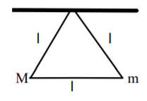
Determine the angular frequency of small oscillations.
Use your result from part (a) to show for .
Show that your result from part (a) agrees with where is the equilibrium angle and is the moment of inertia.
Assume the system has energy . Setup an integral that determines the period of oscillation.
An unusual pendulum is made by fixing a string to a horizontal cylinder of radius , wrapping the string several times around the cylinder, and then tying a mass to the loose end. In equilibrium the mass hangs a distance vertically below the edge of the cylinder. Find the potential energy if the pendulum has swung to an angle from the vertical. Show that for small angles, it can be written in the Hooke’s Law form . Comment of the value of .
Consider the two-dimensional anisotropic oscillator with motion with and .
Prove that if the ratio of the frequencies is rational (that is, where and are integers) then the motion is periodic. What is the period?
Prove that if the same ratio is irrational, the motion never repeats itself.
A simple pendulum consists of a mass suspended from a fixed point by a weight-less, extensionless rod of length .
Obtain the equation of motion, and in the approximation , show that the natural frequency is , where is the gravitational field strength.
Discuss the motion in the event that the motion takes place in a viscous medium with retarding force .
Derive the expression for the State Space paths of the plane pendulum if the total energy is . Note that this is just the case of a particle moving in a periodic potential . Sketch the State Space diagram for both and .
Consider the motion of a driven linearly-damped harmonic oscillator after the transient solution has died out, and suppose that it is being driven close to resonance, .
Show that the oscillator’s total energy is .
Show that the energy dissipated during one cycle by the damping force is
Two masses and slide freely on a horizontal frictionless rail and are connected by a spring whose force constant is k. Find the frequency of oscillatory motion for this system.
A particle of mass moves under the influence of a resistive force proportional to velocity and a potential , that is .
where and
Find the points of stable and unstable equilibrium.
Find the solution of the equations of motion for small oscillations around the stable equilibrium points
Show that as the particle approaches one of the stable equilibrium points for most choices of initial conditions. What are the exceptions? (Hint: You can prove this without finding the solutions explicitly.)
3.S: Linear Oscillators (Summary)
Linear systems have the feature that the solutions obey the Principle of Superposition, that is, the amplitudes add linearly for the superposition of different oscillatory modes. Applicability of the Principle of Superposition to a system provides a tremendous advantage for handling and solving the equations of motion of oscillatory systems.
Geometric representations of the motion of dynamical systems provide sensitive probes of periodic motion. Configuration space , state space and phase space , are powerful geometric representations that are used extensively for recognizing periodic motion where , , and are vectors in -dimensional space.
Linearly-damped free linear oscillator
The free linearly-damped linear oscillator is characterized by the equation
The solutions of the linearly-damped free linear oscillator are of the form
The solutions fall into three categories
underdamped | ||
overdamped | ||
critically damped |
The energy dissipation for the linearly-damped free linear oscillator time averaged over one period is given by
The quality factor characterizing the damping of the free oscillator is define to be
where is the energy dissipated per radian.
Sinusoidally-driven, linearly-damped, linear oscillator
The linearly-damped linear oscillator, driven by a harmonic driving force, is of considerable importance to all branches of physics, and engineering. The equation of motion can be written as
where is the driving force. The complete solution of this second-order differential equation comprises two components, the complementary solution (transient response), and the particular solution (steady-state response). That is,
For the underdamped case, the transient solution is the complementary solution
and the steady-state solution is given by the particular solution
Resonance
A detailed discussion of resonance and energy absorption for the driven linearly-damped linear oscillator was given. For resonance the maximum amplitudes occur at frequencies
Resonant system | Resonant frequency |
undamped free linear oscillator | |
linearly-damped free linear oscillator | |
driven linearly-damped linear oscillator |
The energy absorption for the steady-state solution for resonance is given by
where the elastic amplitude
while the absorptive amplitude
The time average power input is given by only the absorptive term
This power curve has the classic Lorentzian shape.
Wave propagation
The wave equation was introduced and both traveling and standing wave solutions of the wave equation were discussed. Harmonic wave-form analysis, and the complementary time-sampled wave form analysis techniques, were introduced in this chapter and in appendix 19.9. The relative merits of Fourier analysis and the digital Green’s function waveform analysis were illustrated for signal processing.
The concepts of phase velocity, group velocity, and signal velocity were introduced. The phase velocity is given by
and group velocity
If the group velocity is frequency dependent then the information content of a wave packet travels at the signal velocity which can differ from the group velocity.
The Wave-packet Uncertainty Principle implies that making a precise measurement of the frequency of a sinusoidal wave requires that the wave packet be infinitely long. The standard deviation characterizing the width of the amplitude of the wavepacket spectral distribution in the angular frequency domain, , and the corresponding width in time , are related by :
The standard deviations for the spectral distribution and width of the intensity of the wave packet are related by:
This applies to all forms of wave motion, including sound waves, water waves, electromagnetic waves, or matter waves.
A universal name for the representation has not been adopted in the literature. Therefore this book has adopted the name “state space”. Lanczos [La49] uses the term “state space” to refer to the extended phase space discussed in chapter 17.