13. Rigid-body Rotation

13.1: Introduction to Rigid-body Rotation¶

Rigid-body rotation features prominently in science, engineering, and sports. Prior chapters have focussed primarily on motion of point particles. This chapter extends the discussion to motion of finite-sized rigid bodies. A rigid body is a collection of particles where the relative separations remain rigidly fixed. In real life, there is always some motion between individual atoms, but usually this microscopic motion can be neglected when describing macroscopic properties. Note that the concept of perfect rigidity has limitations in the theory of relativity since information cannot travel faster than the velocity of light, and thus signals cannot be transmitted instantaneously between the ends of a rigid body which is implied if the body had perfect rigidity.

The description of rigid-body rotation is most easily handled by specifying the properties of the body in the rotating body-fixed coordinate frame whereas the observables are measured in the stationary inertial laboratory coordinate frame. In the body-fixed coordinate frame, the primary observable for classical mechanics is the inertia tensor of the rigid body which is well defined and independent of the rotational motion. By contrast, in the stationary inertial frame the observables depend sensitively on the details of the rotational motion. For example, when observed in the stationary fixed frame, rapid rotation of a long thin cylindrical pencil about the longitudinal symmetry axis gives a time-averaged shape of the pencil that looks like a thin cylinder, whereas the time-averaged shape is a flat disk for rotation about an axis perpendicular to the symmetry axis of the pencil. In spite of this, the pencil always has the same unique inertia tensor in the body-fixed frame. Thus the best solution for describing rotation of a rigid body is to use a rotation matrix that transforms from the stationary fixed frame to the instantaneous body-fixed frame for which the moment of inertia tensor can be evaluated. Moreover, the problem can be greatly simplified by transforming to a body-fixed coordinate frame that is aligned with any symmetry axes of the body since then the inertia tensor can be diagonal; this is called a principal axis system.

Rigid-body rotation can be broken into the following two classifications.

1) Rotation about a fixed axis:¶

A body can be constrained to rotate about an axis that has a fixed location and orientation relative to the body. The hinged door is a typical example. Rotation about a fixed axis is straightforward since the axis of rotation, plus the moment of inertia about this axis, are well defined and this case was discussed in chapter $(2.12)$ .

2) Rotation about a point¶

A body can be constrained to rotate about a fixed point of the body but the orientation of this rotation axis about this point is unconstrained. One example is rotation of an object flying freely in space which can rotate about the center of mass with any orientation. Another example is a child’s spinning top which has one point constrained to touch the ground but the orientation of the rotation axis is undefined.

The prior discussion in chapter $(2.12)$ showed that rigid-body rotation is more complicated than assumed in introductory treatments of rigid-body rotation. It is necessary to expand the concept of moment of inertia to the concept of the inertia tensor, plus the fact that the angular momentum may not point along the rotation axis. The most general case requires consideration of rotation about a body-fixed point where the orientation of the axis of rotation is unconstrained. The concept of the inertia tensor of a rotating body is crucial for describing rigid-body motion. It will be shown that working in the body-fixed coordinate frame of a rotating body allows a description of the equations of motion in terms of the inertia tensor for a given point of the body, and that it is possible to rotate the body-fixed coordinate system into a principal axis system where the inertia tensor is diagonal. For any principal axis, the angular momentum is parallel to the angular velocity if it is aligned with a principal axis. The use of a principal axis system greatly simplifies treatment of rigid-body rotation and exploits the powerful and elegant matrix algebra mentioned in appendix 19.1.

The following discussion of rigid-body rotation is broken into three topics, (1) the inertia tensor of the rigid body, (2) the transformation between the rotating body-fixed coordinate system and the laboratory frame, i.e., the Euler angles specifying the orientation of the body-fixed coordinate frame with respect to the laboratory frame, and (3) Lagrange and Euler’s equations of motion for rigid-bodies. This is followed by a discussion of practical applications.

13.2: Rigid-body Coordinates¶

Motion of a rigid body is a special case for motion of the $N$ -body system when the relative positions of the $N$ bodies are related. It was shown in chapter 2 that the motion of a rigid body can be broken into a combination of a linear translation of some point in the body, plus rotation of the body about an axis through that point. This is called Chasles’ Theorem. Thus the position of every particle in the rigid body is fixed with respect to one point in the body. If the fixed point of the body is chosen to be the center of mass, then, as discussed in chapter 2, it is possible to separate the kinetic energy, linear momentum, and angular momentum into the center-of-mass motion, plus the motion about the center of mass. Thus the behavior of the body can be described completely using only six independent coordinates governed by six equations of motion, three for translation and three for rotation.

Referred to an inertial frame, the translational motion of the center of mass is governed by

\mathbf{F}^{E} = \frac{d\mathbf{P}}{dt}

while the rotational motion about the center of mass is determined by

\mathbf{N}^{E} = \frac{d\mathbf{L}}{dt}

where the external force $\mathbf{F}^{E}$ and external torque $\mathbf{N}^{E}$ are identified separately from the internal forces acting between the particles in the rigid body. It will be assumed that the internal forces are central and thus do not contribute to the angular momentum.

The location of any fixed point in the body, such as the center of mass, can be specified by three generalized cartesian coordinates with respect to a fixed frame. The rotation of the body-fixed axis system about this fixed point in the body can be described in terms of three independent angles with respect to the fixed frame. There are several possible sets of orthogonal angles that can be used to describe the rotation. This book uses the Euler angles $\phi, \theta, \psi$ which correspond first to a rotation $\phi$ about the $z$ -axis, then a rotation $\theta$ about the $x$ axis subsequent to the first rotation, and finally a rotation $\psi$ about the new $z$ axis following the first two rotations. The Euler angles will be discussed in detail following introduction of the inertia tensor and angular momentum.

13.3: Rigid-body Rotation about a Body-Fixed Point¶

With respect to some point $O$ fixed in the body coordinate system, the angular momentum of the body $\alpha$ is given by

\mathbf{L} = \sum^{n}_i \mathbf{L}_i = \sum^n_i \mathbf{r}_i \times \mathbf{p}_i

There are two especially convenient choices for the fixed point $O$ . If no point in the body is fixed with respect to an inertial coordinate system, then it is best to choose $O$ as the center of mass. If one point of the body is fixed with respect to a fixed inertial coordinate system, such as a point on the ground where a child’s spinning top touches, then it is best to choose this stationary point as the body-fixed point $O$ .

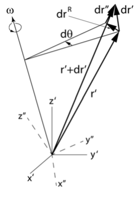
Infinitessimal displacement dr^{\prime} in the primed frame, broken into a part dr^R due to rotation of the primed frame plus a part dr^{\prime\prime} due to displacement with respect to this rotating frame. — Figure 13.3.1:Infinitessimal displacement $dr^{\prime}$ in the primed frame, broken into a part $dr^R$ due to rotation of the primed frame plus a part $dr^{\prime\prime}$ due to displacement with respect to this rotating frame.

Consider a rigid body composed of $N$ particles of mass $m_{\alpha}$ where $\alpha = 1, 2, 3, \dots N$ . As discussed in chapter 12.4, if the body rotates with an instantaneous angular velocity $\boldsymbol{\omega}$ about some fixed point, with respect to the body-fixed coordinate system, and this point has an instantaneous translational velocity $\mathbf{V}$ with respect to the fixed (inertial) coordinate system, see Figure 13.3.1, then the instantaneous velocity $\mathbf{v}_{\alpha}$ of the $\alpha^{th}$ particle in the fixed frame of reference is given by

\mathbf{v}_{\alpha} = \mathbf{V} + \mathbf{v}^{\prime\prime}_{\alpha} + \boldsymbol{\omega} \times \mathbf{r}^{\prime}_{\alpha}

However, for a rigid body, the velocity of a body-fixed point with respect to the body is zero, that is $\mathbf{v}^{\prime\prime}_{\alpha} = 0$ , thus

\mathbf{v}_{\alpha} = \mathbf{V} + \boldsymbol{\omega} \times \mathbf{r}^{\prime}_{ \alpha}

Consider the translational velocity of the body-fixed point $O$ to be zero, i.e. $\mathbf{V} = 0$ and let $\mathbf{R} = 0$ , then $\mathbf{r}_{\alpha} = \mathbf{r}^{\prime}_{\alpha}$ . These assumptions allow the linear momentum of the particle $\alpha$ to be written as

\mathbf{p}_{\alpha} = m_{\alpha} \mathbf{v}_{\alpha} = m_{\alpha} \boldsymbol{\omega} \times \mathbf{ r}_{\alpha}

Therefore

\mathbf{L} = \sum^N_{\alpha} \mathbf{r}_{\alpha} \times \mathbf{ p}_{\alpha} = \sum^N_{\alpha} m_{\alpha} \mathbf{r}_{\alpha} \times (\boldsymbol{\omega} \times\mathbf{ r}\alpha )

Using the vector identity

\mathbf{A} \times (\mathbf{B} \times \mathbf{ A}) = A^2\mathbf{B} − \mathbf{A} (\mathbf{A} \cdot \mathbf{B}) \notag

leads to

\mathbf{L} = \sum^{N}_{\alpha} m_{\alpha} [r^2_{\alpha} \boldsymbol{\omega} − \mathbf{r}_{\alpha} (\mathbf{r}_{\alpha} \cdot \boldsymbol{\omega}) ]

The angular momentum can be expressed in terms of components of $\boldsymbol{\omega}$ and $\mathbf{r}^{\prime}_{\alpha}$ relative to the body-fixed frame. The following formulae can be written more compactly if $\mathbf{r}_{\alpha} = (x_{\alpha }, y_{\alpha} , z_{\alpha} )$ , in the rotating body-fixed frame, is written in the form $\mathbf{r}_{\alpha} = (x_{\alpha ,1}, y_{\alpha ,2} , z_{\alpha ,3} )$ where the axes are defined by the numbers $1, 2, 3$ rather than $x, y, z$ . In this notation, the angular momentum is written in component form as

L_{i}=\sum_{\alpha}^{N} m_{\alpha}\left[\omega_{i} \sum_{k} x_{\alpha, k}^{2}-x_{\alpha, i}\left(\sum_{j} x_{\alpha, j} \omega_{j}\right)\right] \tag{13.9}

Assume the Kronecker delta relation

\omega_i = \sum^3_j \omega_j \delta_{ij} \tag{13.10}

where

\begin{aligned} \delta_{ij} & = & 1 && i=j \\ \delta_{ij} & = & 0 && i \neq j \end{aligned}

Substitute 13.10 in 13.9 gives

\begin{align} L_{i} &=\sum_{\alpha}^{N} m_{\alpha} \sum_{j}\left[\omega_{j} \delta_{i j} \sum_{k} x_{\alpha, k}^{2}-\omega_{j} x_{\alpha, i} x_{\alpha, j}\right] \notag \\ &=\sum_{j}^{3} \omega_{j}\left[\sum_{\alpha}^{N} m_{\alpha}\left(\delta_{i j} \sum_{k} x_{\alpha, k}^{2}-x_{\alpha, i} x_{\alpha, j}\right)\right] \end{align}

13.4: Inertia Tensor¶

The square bracket term in $(13.3.9)$ is called the moment of inertia tensor, $\mathbf{I}$ , which is usually referred to as the inertia tensor

I_{ij} \equiv \sum^{N}_{\alpha} m_{\alpha} \left[ \delta_{ij} \left( \sum^3_k x^2_{\alpha , k} \right) − x_{\alpha , i} x_{\alpha , j} \right] \tag{13.12}

In most cases it is more useful to express the components of the inertia tensor in an integral form over the mass distribution rather than a summation for $N$ discrete bodies. That is,

I_{ij} = \int\rho (\mathbf{r}^{\prime} ) \left( \delta_{ij} \left( \sum^3_k x^2_{k} \right) − x_{i} x_{ j} \right) dV

The inertia tensor is easier to understand when written in cartesian coordinates $\mathbf{r}^{\prime}_{\alpha} = (x_{\alpha}, y_{\alpha}, z_{\alpha})$ rather than in the form $\mathbf{r}^{\prime}_{\alpha} = (x_{\alpha ,1}, x_{\alpha ,2}, x_{\alpha ,3})$ . Then, the diagonal moments of inertia of the inertia tensor are

\begin{align} I_{x x} & \equiv \sum_{\alpha}^{N} m_{\alpha}\left[x_{\alpha}^{2}+y_{\alpha}^{2}+z_{\alpha}^{2}-x_{\alpha}^{2}\right]=\sum_{\alpha}^{N} m_{\alpha}\left[y_{\alpha}^{2}+z_{\alpha}^{2}\right] \\[4pt] \notag I_{y y} & \equiv \sum_{\alpha}^{N} m_{\alpha}\left[x_{\alpha}^{2}+y_{\alpha}^{2}+z_{\alpha}^{2}-y_{\alpha}^{2}\right]=\sum_{\alpha}^{N} m_{\alpha}\left[x_{\alpha}^{2}+z_{\alpha}^{2}\right] \\[4pt] I_{z z} & \equiv \sum_{\alpha}^{N} m_{\alpha}\left[x_{\alpha}^{2}+y_{\alpha}^{2}+z_{\alpha}^{2}-z_{\alpha}^{2}\right]=\sum_{\alpha}^{N} m_{\alpha}\left[x_{\alpha}^{2}+y_{\alpha}^{2}\right] \notag \end{align}

while the off-diagonal products of inertia are

\begin{align} I_{yx} & = I_{xy} \equiv - \sum^N_{\alpha} m_{\alpha} [x_{\alpha} y_{\alpha}] \\[4pt] \notag I_{zx} & = I_{xz} \equiv - \sum^N_{\alpha} m_{\alpha} [x_{\alpha} z_{\alpha}] \\[4pt] \notag I_{zy} & = I_{yz} \equiv - \sum^N_{\alpha} m_{\alpha} [y_{\alpha} z_{\alpha}] \end{align}

Note that the products of inertia are symmetric in that

I_{ij} = I_{ji}

The above notation for the inertia tensor allows the angular momentum 13.12 to be written as

L_i = \sum^3_j I_{ij} \omega_j

Expanded in cartesian coordinates

\begin{align} L_x & = I_{xx} \omega_x + I_{xy} \omega_y + I_{xz} \omega_z \\[4pt] \notag L_y & = I_{yx} \omega_x + I_{yy} \omega_y + I_{yz} \omega_z \\[4pt] \notag L_z & = I_{zx} \omega_x + I_{zy} \omega_y + I_{zz} \omega_z \end{align}

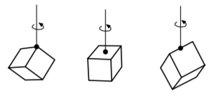
Note that every fixed point in a body has a specific inertia tensor. The components of the inertia tensor at a specified point depend on the orientation of the coordinate frame whose origin is located at the specified fixed point. For example, the inertia tensor for a cube is very different when the fixed point is at the center of mass compared with when the fixed point is at a corner of the cube.

13.5: Matrix and Tensor Formulations of Rigid-Body Rotation¶

The prior notation is clumsy and can be streamlined by use of matrix methods. Write the inertia tensor in a matrix form as

\{\mathbb{I}\}= \begin{pmatrix} I_{11} & I_{12} & I_{13} \\ I_{21} & I_{22} & I_{23} \\ I_{31} & I_{32} & I_{33} \end{pmatrix}

The angular velocity and angular momentum both can be written as a column vectors, that is

$$ \boldsymbol{\omega}=\begin{pmatrix} \omega_{1} \ \omega_{2} \ \omega_{3}

\end{pmatrix} \quad \mathbf{L}=\begin{pmatrix} L_{1} \ L_{2} \ L_{3} \end{pmatrix} $$

As discussed in appendix 19.5.2, Equation 13.4.7 now can be written in tensor notation as an inner product of the form

L = \{\mathbb{I}\} \cdot \boldsymbol{\omega}

Note that the above notation uses boldface for the inertia tensor $\mathbb{I}$ , implying a rank-2 tensor representation, while the angular velocity $\boldsymbol{\omega}$ and the angular momentum $\mathbf{L}$ are written as column vectors. The inertia tensor is a 9-component rank-2 tensor defined as the ratio of the angular momentum vector $\mathbf{L}$ and the angular velocity $\boldsymbol{\omega}$ .

\{\mathbb{I}\} = \frac{\mathbf{L}}{\boldsymbol{\omega}}

Note that, as described in appendix 19.5, the inner product of a vector $\boldsymbol{\omega}$ , which is the rank 1 tensor, and a rank 2 tensor $\{\mathbb{I}\}$ , leads to the vector $\mathbf{L}$ . This compact notation exploits the fact that the matrix and tensor representation are completely equivalent, and are ideally suited to the description of rigid-body rotation.

13.6: Principal Axis System¶

The inertia tensor is a real symmetric matrix because of the symmetry given by equation $(13.4.5)$ . A property of real symmetric matrices is that there exists an orientation of the coordinate frame, with its origin at the chosen body-fixed point $O$ , such that the inertia tensor is diagonal. The coordinate system for which the inertia tensor is diagonal is called the Principal axis system which has three perpendicular principal axes. Thus, in the principal axis system, the inertia tensor has the form

\{\mathbf{I}\} = \begin{pmatrix} I_{11} & 0 & 0 \\ 0 & I_{22} & 0 \\ 0 & 0 & I_{33} \end{pmatrix}

where $I_{ij}$ are real numbers, which are called the principal moments of inertia of the body, and are usually written as $I_j$ . When the angular velocity vector $\boldsymbol{\omega}$ points along any principal axis unit vector $\hat{j}$ , then the angular momentum $\mathbf{L}$ is parallel to $\boldsymbol{\omega}$ and the magnitude of the principal moment of inertia about this principal axis is given by the relation

L_j \hat{j} = I_j \omega_j \hat{j} \tag{13.24}

The principal axes are fixed relative to the shape of the rigid body and they are invariant to the orientation of the body-fixed coordinate system used to evaluate the inertia tensor. The advantage of having the bodyfixed coordinate frame aligned with the principal axis coordinate frame is that then the inertia tensor is diagonal, which greatly simplifies the matrix algebra. Even when the body-fixed coordinate system is not aligned with the principal axis frame, if the angular velocity is specified to point along a principal axis then the corresponding moment of inertia will be given by 13.24.

In principle it is possible to locate the principal axes by varying the orientation of the angular velocity vector $\boldsymbol{\omega}$ to find those orientations for which the angular momentum $\mathbf{L}$ and angular velocity $\boldsymbol{\omega}$ are parallel which characterizes the principal axes. However, the best approach is to diagonalize the inertia tensor.

13.7: Diagonalize the Inertia Tensor¶

Finding the three principal axes involves diagonalizing the inertia tensor, which is the classic eigenvalue problem discussed in appendix 19.1. Solution of the eigenvalue problem for rigid-body motion corresponds to a rotation of the coordinate frame to the principal axes resulting in the matrix

\{\mathbf{I}\} \cdot \boldsymbol{\omega} = I\boldsymbol{\omega}

where $I$ comprises the three-valued eigenvalues, while the corresponding vector $\boldsymbol{\omega}$ is the eigenvector. Appendix 19.1 gives the solution of the matrix relation

\{\mathbf{I}\} \cdot \boldsymbol{\omega} = I \{\mathbb{I}\} \boldsymbol{\omega} \tag{13.26}

where $I$ are three-valued eigen values for the principal axis moments of inertia, and $\{\mathbb{I}\}$ is the unity tensor, equation $(A.2.4)$ .

\{\mathbb{I}\} \equiv \begin{Bmatrix} 1 & 0 & 0 \\ 0 & 1 & 0 \\ 0 & 0 & 1 \end{Bmatrix}

Rewriting 13.26 gives

(\{\mathbf{I}\} − I \{\mathbb{I}\}) \cdot \boldsymbol{\omega} = 0 \tag{13.28}

This is a matrix equation of the form $\mathbf{A} \cdot \boldsymbol{\omega} =0$ where $\mathbf{A}$ is a $3 \times 3$ matrix and $\boldsymbol{\omega}$ is a vector with values $\omega_x , \omega_y, \omega_z$ . The matrix equation $\mathbf{A} \cdot \boldsymbol{\omega} =0$ really corresponds to three simultaneous equations for the three numbers $\omega_x , \omega_y, \omega_z$ . It is a well-known property of equations like 13.28 that they have a non-zero solution if, and only if, the determinant $\text{det}(\mathbf{A})$ is zero, that is

\text{det}(\mathbf{I}−I\mathbb{I})=0

This is called the characteristic equation, or secular equation for the matrix $\mathbf{I}$ . The determinant involved is a cubic equation in the value of $I$ that gives the three principal moments of inertia. Inserting one of the three values of $I$ into equation $(13.4.6)$ gives the corresponding eigenvector $\omega$ . Applying the above eigenvalue problem to rigid-body rotation corresponds to requiring that some arbitrary set of body-fixed axes be the principal axes of inertia. This is obtained by rotating the body-fixed axis system such that

\begin{align} L_1 & = & I_{11}\omega_1 + I_{12}\omega_2 + I_{13}\omega_3 = I\omega_1 \\ L_2 & = & I_{21}\omega_1 + I_{22}\omega_2 + I_{23}\omega_3 = I\omega_2 \notag \\ L_3 & = & I_{31}\omega_1 + I_{32}\omega_2 + I_{33}\omega_3 = I\omega_3 \notag \end{align}

\begin{align}(I_{11} − I) \omega_1 + I_{12}\omega_2 + I_{13}\omega_3 = 0 \\ I_{21}\omega_1 + (I_{22} − I) \omega_2 + I_{23}\omega_3 = 0 \notag \\ I_{31}\omega_1 + I_{32}\omega_2 + (I_{33} − I) \omega_3 = 0 \notag \end{align}

These equations have a non-trivial solution for the ratios $\omega_1 : \omega_2 : \omega_3$ since the determinant vanishes, that is

\begin{vmatrix} (I_{11} − I) & I_{12} & I_{13} \\ I_{21} & (I_{22} − I) & I_{23} \\ I_{31} & I_{32} & (I_{33} − I) \end{vmatrix} = 0

The expansion of this determinant leads to a cubic equation with three roots for $I$ . This is the secular equation for $I$ whose eigenvalues are the principal moments of inertia.

The directions of the principal axes, that is the eigenvectors, can be found by substituting the corresponding solution for $I$ into the prior equation. Thus for eigensolution $I_1$ the eigenvector is given by solving

\begin{align}(I_{11} − I_1) \omega_{11} + I_{12}\omega_{21} + I_{13}\omega_{31} = 0 \\ I_{21}\omega_{11} + (I_{22} − I_1) \omega_{21} + I_{23}\omega_{31} = 0 \notag \\ I_{31}\omega_{11} + I_{32}\omega_{21} + (I_{33} − I_1) \omega_{31} = 0 \notag \end{align}

These equations are solved for the ratios $\omega_{11} : \omega_{21} : \omega_{31}$ which are the direction numbers of the principle axis system corresponding to solution $I_1$ . This principal axis system is defined relative to the original coordinate system. This procedure is repeated to find the orientation of the other two mutually perpendicular principal axes.

13.8: Parallel-Axis Theorem¶

The values of the components of the inertia tensor depend on both the location and the orientation about which the body rotates relative to the body-fixed coordinate system. The parallel-axis theorem is valuable for relating the inertia tensor for rotation about parallel axes passing through different points fixed with respect to the rigid body. For example, one may wish to relate the inertia tensor through the center of mass to another location that is constrained to remain stationary, like the tip of the spinning top.

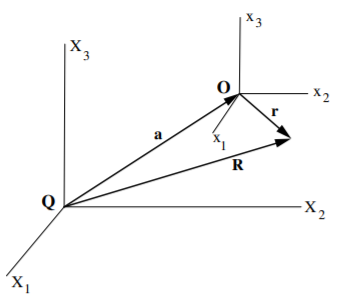
Figure 13.8.1:Transformation between two parallel body-coordinate systems, O and Q.

Consider the mass ${\alpha}$ at the location $\mathbf{r} = (x_1, x_2, x_3)$ with respect to the origin of the center of mass body-fixed coordinate system $O$ . Transform to an arbitrary but parallel body-fixed coordinate system $Q$ , that is, the coordinate axes have the same orientation as the center of mass coordinate system. The location of the mass ${\alpha}$ with respect to this arbitrary coordinate system is $\mathbf{R} = (X_1, X_2, X_3)$ . That is, the general vectors for the two coordinates systems are related by

\mathbf{R} = \mathbf{a} + \mathbf{r} \tag{13.34}

where $\mathbf{a}$ is the vector connecting the origins of the coordinate systems $O$ and $Q$ illustrated in Figure 13.8.1. The elements of the inertia tensor with respect to axis system $Q$ , are given by equation $(13.4.1)$ to be

J_{i j} \equiv \sum_{\alpha}^{N} m_{\alpha}\left[\delta_{i j}\left(\sum_{k}^{3} X^2_{\alpha, k} \right) - X_{\alpha, i}X_{\alpha, j} \right]

The components along the three axes for each of the two coordinate systems are related by

X_i = a_i + x_i

Substituting these into the above inertia tensor relation gives

\begin{align} J_{i j} &=\sum_{\alpha}^{N} m_{\alpha}\left[\delta_{i j}\left(\sum_{k}^{3}\left(x_{\alpha, k}+a_{i}\right)^{2}\right)-\left(x_{\alpha, i}+a_{i}\right)\left(x_{\alpha, j}+a_{i}\right)\right] \\ &=\sum_{\alpha}^{N} m_{\alpha}\left[\delta_{i j}\left(\sum_{k}^{3} x_{\alpha, k}^{2}\right)-x_{\alpha, i} x_{\alpha, j}\right]+\sum_{\alpha}^{N} m_{\alpha}\left[\delta_{i j}\left(\sum_{k}^{3}\left(2 x_{\alpha, k} a_{k}+a_{k}^{2}\right)\right)-\left(a_{i} x_{\alpha, j}+a_{j} x_{\alpha, i}+a_{i} a_{j}\right)\right] \notag \end{align}

The first summation on the right-hand side corresponds to the elements $I_{ij}$ of the inertia tensor in the center-of-mass frame. Thus the terms can be regrouped to give

J_{i j} \equiv I_{ij} + \sum_{\alpha}^{N} m_{\alpha} \left( \delta_{ij} \sum^3_k a^2_k - a_{i}a_j \right) + \sum_{\alpha}^{N} m_{\alpha}\left[2\delta_{i j} \sum_{k}^{3} x_{\alpha, k} a_{k} - a_i x_{\alpha, j} - a_{j} x_{\alpha, i} \right]

However, each term in the last bracket involves a sum of the form $\sum^N_{\alpha} m_{\alpha} x_{\alpha ,k}$ . Take the coordinate system $O$ to be with respect to the center of mass for which

\sum^N_{\alpha} m_{\alpha} \mathbf{r}^{\prime} = 0

This also applies to each component $k$ , that is

\sum^N_{\alpha} m_{\alpha} x_{\alpha ,k} = 0

Therefore all of the terms in the last bracket cancel leaving

J_{i j} \equiv I_{ij} + \sum_{\alpha}^{N} m_{\alpha} \left( \delta_{ij} \sum^3_k a^2_k - a_{i}a_j \right)

But $\sum^N_{\alpha} m_{\alpha} = M$ and $\sum^3_k a^2_k = a^2$ , thus

J_{ij} \equiv I_{ij} +M (a^2\delta_{ij} - a_ia_j)

where $I_{ij}$ is the center-of-mass inertia tensor. This is the general form of Steiner’s parallel-axis theorem.

As an example, the moment of inertia around the $X_1$ axis is given by

J_{11} \equiv I_{11} + M((a^2_1 + a^2_2 + a^3_3) \delta_{11} - a^2_1) = I_{11} + M(a^2_2 + a^2_3)

which corresponds to the elementary statement that the difference in the moments of inertia equals the mass of the body multiplied by the square of the distance between the parallel axes, $x_1, X_1$ . Note that the minimum moment of inertia of a body is $I_{ij}$ which is about the center of mass.

Example 13.8.1: Inertia Tensor of a Solid Cube Rotating about the Center of Mass

The complicated expressions for the inertia tensor can be understood using the example of a uniform solid cube with side $b$ , density $\rho$ , and mass $M = \rho b^3$ , rotating about different axes. Assume that the origin of the coordinate system $O$ is at the center of mass with the axes perpendicular to the centers of the faces of the cube.

Figure 13.8.2:Inertia tensor of a uniform solid cube of side $b$ about the center of mass $O$ and a corner of the cube $Q$ . The vector $a$ is the vector distance between $O$ and $Q$ .

The components of the inertia tensor can be calculated using $(13.4.2)$ written as an integral over the mass distribution rather than a summation.

I_{ij} = \int \rho ( \mathbf{r}^{\prime} ) \left(\delta_{ij} \left( \sum^3_k x^2_k \right) -x_ix_j\right) dV \nonumber

Thus

\begin{align*} I_{11} & = \rho \int^{b/2}_{-b/2} \int^{b/2}_{-b/2} \int^{b/2}_{-b/2} (x^2_2 + x^2_3) dx_3 dx_2 dx_1 \\[4pt] & = \frac{1}{6} \rho b^5 = \frac{1}{6} Mb^2 = I_{22} = I_{33} \end{align*}

By symmetry the diagonal moments of inertia about each face are identical. Similarly the products of inertia are given by

I_{12} = -\rho \int^{b/2}_{-b/2} \int^{b/2}_{-b/2} \int^{b/2}_{-b/2} (x_1x_2) dx_3 dx_2 dx_1 = 0\notag

Thus the inertia tensor is given by

\mathbf{I}^{cm} = \frac{1}{6} Mb^2 \begin{pmatrix} 1 & 0 & 0 \\ 0 & 1 & 0 \\ 0 & 0 & 1 \end{pmatrix} \notag

Note that this inertia tensor is diagonal implying that this is the principal axis system. In this case all three principal moments of inertia are identical and perpendicular to the centers of the faces of the cube. This is as expected from the symmetry of the cubic geometry.

Example 13.8.2: Inertia tensor of about a corner of a solid cube.

Direct calculation¶

Let one corner of the cube be the origin of the coordinate system $Q$ and assume that the three adjacent sides of the cube lie along the coordinate axes. The components of the inertia tensor can be calculated using $(13.4.2)$ . Thus

I_{11} = \rho \int^b_0 \int^b_0 \int^b_0 (x^2_2 + x^2_3) dx_3 dx_2 dx_1 = \frac{2}{3} \rho b^5 = \frac{2}{3} Mb^2 \notag

I_{12} = \rho \int^b_0 \int^b_0 \int^b_0 (x_1 x_2) dx_3 dx_2 dx_1 = -\frac{1}{4} \rho b^5 = - \frac{1}{4} Mb^2 \notag

Thus, evaluating all the nine components gives

\mathbf{I}^{corner} = \frac{1}{12} Mb^2 \begin{pmatrix} 8 & -3 & -3 \\ -3 & 8 & -3 \\ -3 & -3 & 8 \end{pmatrix} \nonumber

Parallel-axis theorem¶

This inertia tensor also can be calculated using the parallel-axis theorem to relate the moment of inertia about the corner, to that at the center of mass. As shown in Figure 13.8.2, the vector $a$ has components

a_1 = a_2 = a_3 = \frac{b}{2}\nonumber

Applying the parallel-axis theorem gives

J_{11} = I_{11} + M ( a^2 − a^2_1) = I_{11} + M ( a^2_2 + a^2_3) = \frac{1}{6} Mb^2 + \frac{1}{2} Mb^2 = \frac{2}{3} Mb^2 \nonumber

and similarly for $J_{22}$ and $J_{33}$ . The off-diagonal terms are given by

J_{12} = I_{12} + M (−a_1a_2) = −\frac{1}{4}Mb^2 \nonumber

Thus the inertia tensor, transposed from the center of mass, to the corner of the cube is

\mathbf{I}^{corner} = \begin{pmatrix} \frac{2}{3} Mb^2 & -\frac{1}{4} Mb^2 & -\frac{1}{4} Mb^2 \\ -\frac{1}{4}Mb^2 & \frac{2}{3} Mb^2 & -\frac{1}{4} Mb^2\\ -\frac{1}{4} Mb^2 & -\frac{1}{4} Mb^2 & \frac{2}{3} Mb^2\end{pmatrix} = \frac{1}{12} Mb^2 \begin{pmatrix} 8 & -3 & -3 \\ -3 & 8 & -3 \\ -3 & -3 & 8 \end{pmatrix} \nonumber

This inertia tensor about the corner of the cube, is the same as that obtained by direct integration.

Principal moments of inertia¶

The coordinate axis frame used for rotation about the corner of the cube is not a principal axis frame. Therefore let us diagonalize the inertia tensor to find the principal axis frame and the principal moments of inertia about a corner. To achieve this requires solving the secular determinant

\begin{vmatrix} (\frac{2}{3} Mb^2 - I) & -\frac{1}{4} Mb^2 & -\frac{1}{4} Mb^2 \\ -\frac{1}{4} Mb^2 & (\frac{2}{3} Mb^2 - I) & -\frac{1}{4} Mb^2\\ -\frac{1}{4} Mb^2 & -\frac{1}{4} Mb^2 & (\frac{2}{3} Mb^2 - I) \end{vmatrix} = 0 \notag

The value of a determinant is not affected by adding or subtracting any row or column from any other row or column. Subtract row 1 from row 2 gives

\begin{vmatrix} (\frac{2}{3} Mb^2 - I) & -\frac{1}{4} Mb^2 & -\frac{1}{4} Mb^2 \\ -\frac{11}{12} Mb^2 & (\frac{11}{12} Mb^2 - I) & 0 \\ -\frac{1}{4} Mb^2 & -\frac{1}{4} Mb^2 & (\frac{2}{3} Mb^2 - I) \end{vmatrix} = 0 \notag

The determinant of this matrix is straightforward to evaluate and equals

\left(\frac{1}{6}Mb^2 - I \right) \left( \frac{11}{12}Mb^2 - I\right) \left(\frac{11}{12}Mb^2 - I \right) = 0 \nonumber

Thus the roots are

\mathbf{I}^{corner} = \begin{pmatrix} \frac{1}{6}Mb^2 & 0 & 0 \\ 0 & \frac{11}{12}Mb^2 & 0 \\ 0 & 0 & \frac{11}{12}Mb^2 \end{pmatrix}\notag

The identical roots $I_{22} = I_{33} = \frac{11}{12} Mb^2$ imply that the principal axis associated with $I_{11}$ must be a symmetry axis. The orientation can be found by substituting $I_{11}$ into the above equation

(\{\mathbf{I}\} − I \{\mathbb{I}\}) \cdot \boldsymbol{\omega} = \frac{1}{12} Mb^2 \begin{pmatrix} 6 & −3 & −3\\ −3& 6 & −3\\ −3 &−3 & 6 \end{pmatrix} \begin{pmatrix} \omega_{11} \\ \omega_{21} \\ \omega_{31} \end{pmatrix} = 0 \notag

where the second subscript 1 attached to $\omega_i$ signifies that this solution corresponds to $I_{11}$ . This gives

\begin{aligned} 2\omega_{11} − \omega_{21} − \omega_{31} = 0 \\ −\omega_{11} + 2\omega_{21} − \omega_{31} = 0 \\ −\omega_{11} − \omega_{21} + 2\omega_{31} = 0 \end{aligned}

Solving these three equations gives the unit vector for the first principal axis for which $I_{11} = \frac{1}{6} Mb^2$ to be $\mathbf{\hat{e}}_1= \frac{1}{\sqrt{3}} \begin{pmatrix} 1 \\ 1 \\ 1 \end{pmatrix}$ . This can be repeated to find the other two principal axes by substituting $I_{22} = \frac{11}{12} Mb^2$ . This gives for the second principal moment $I_{22}$

(\{\mathbf{I}\} − I \{\mathbb{I}\}) \cdot \boldsymbol{\omega} = \frac{1}{12} Mb^2 \begin{pmatrix} −3 & −3 & −3\\ −3& −3& −3\\ −3 &−3 &−3 \end{pmatrix} \begin{pmatrix} \omega_{12} \\ \omega_{22} \\ \omega_{32} \end{pmatrix} = 0 \notag

This results in three identical equations for the components of $\omega$ but all three equations are the same, namely

\omega_{12} + \omega_{22} + \omega_{32} = 0 \notag

This does not uniquely determine the direction of $\omega$ . However, it does imply that $\omega_2$ corresponding to the second principal axis has the property that

\boldsymbol{\hat{\omega}} \cdot \mathbf{\hat{e}}_1 = 0 \notag

that is, any direction of $\hat{e}_2$ that is perpendicular to $\hat{e}_1$ is acceptable. In other words; any two orthogonal unit vectors $\hat{e}_2$ and $\hat{e}_3$ that are perpendicular to $\hat{e}_1$ are acceptable. This ambiguity exists whenever two eigenvalues are equal; the three principal axes are only uniquely defined if all three eigenvalues are different. The same ambiguity exist when all three eigenvalues are identical as occurs for the principal moments of inertia about the center-of-mass of a uniform solid cube. This explains why the principal moment of inertia for the diagonal of the cube, that passes through the center of mass, has the same moment as when the principal axes pass through the center of the faces of the cube.

13.9: Perpendicular-axis Theorem for Plane Laminae¶

Rigid-body rotation of thin plane laminae objects is encountered frequently. Examples of such laminae bodies are a plane sheet of metal, a thin door, a bicycle wheel, a thin envelope or book. Deriving the inertia tensor for a plane lamina is relatively simple because there are limits on the possible relative magnitude of the principal moments of inertia. Consider that the principal axis are along the $x,y,z,$ coordinate axes. Then the sum of two principal moments of inertia about the center of mass are

\begin{align*} I_x + I_y &= \int \rho(y^2 + z^2)dV + \int \rho (x^2 + z^2)dV \\ &= \int \rho(x^2 + y^2)dV + 2 \int \rho z^2 dV \geq \int \rho (x^2 + y^2)dV = I_z \end{align*}

Note that for any body the three principal moments of inertia must satisfy the triangle rule that the sum of any pair must exceed or equal the third. Moreover, if the body is a thin lamina with thickness $z = 0$ , that is, a thin plate in the $x − y$ plane, then

I_x + I_y = I_z \tag{13.45}

This perpendicular-axis theorem can be very useful for solving problems involving rotation of plane laminae.

The opposite of a plane laminae is a long thin cylindrical needle of mass $m$ , length $L$ , and radius $r$ . Along the symmetry axis the principal moments are $I_z = \frac{1}{2}mr^2 \rightarrow 0$ as $r \rightarrow 0$ , while perpendicular to the symmetry axis $I_x = I_y = \frac{1}{12} mL^2$ . These satisfy the triangle rule.

Example 13.9.1: Inertia Tensor of a Hula Hoop

The hula hoop is a thin plane circular ring or radius $R$ and mass $M$ . Assume that the symmetry axis of the circular ring is the 3 axis.

The principal moments of inertia about the center of mass: The principal moment of inertia along the 3 axis is $I_{33} = MR^2$ . Then Equation 13.45 plus symmetry tells us that the two principal moments of inertia in the plane of the hula hoop must be $I_{11} = I_{22} = \frac{1}{2}MR^2$ .
The principal moments of inertia about the periphery of the ring: Using the Parallel-axis theorem tells us that the moment perpendicular to the plane of the hula hoop $I_{33} = 2MR^2$ . In the plane of the hoop the moment tangential to the hoop is $I_{11} = \frac{3}{2} MR^2$ and the moment radial to the hoop $I_{22} = \frac{1}{2}MR^2$ . The hula dancer often swings the hoop about the periphery and perpendicular to the plane by swinging their hips. Another movement is jumping through the hoop by rotating the hoop tangential to the periphery. Calculation of such maneuvers requires knowledge of these principal moments of inertia.

13.10: General Properties of the Inertia Tensor¶

Inertial Equivalence¶

The elements of the inertia tensor, the values of the principal moments of inertia, and the orientation of the principal axes for a rigid body, all depend on the choice of origin for the system. Recall that for the kinetic energy to be separable into translational and rotational portions, the origin of the body coordinate system must coincide with the center of mass of the body. However, for any choice of the origin of any body, there always exists an orientation of the axes that diagonalizes the inertia tensor.

The inertial properties of a body for rotation about a specific body-fixed location is defined completely by only three principal moments of inertia irrespective of the detailed shape of the body. As a result, the inertial properties of any body about a body-fixed point are equivalent to that of an ellipsoid that has the same three principal moments of inertia. The symmetry properties of this equivalent ellipsoidal body define the symmetry of the inertial properties of the body. If a body has some simple symmetry then usually it is obvious as to what will be the principal axes of the body.

Spherical Top: $I_1 = I_2 = I_3$ ¶

A spherical top is a body having three degenerate principal moments of inertia. Such a body has the same symmetry as the inertia tensor about the center of a uniform sphere. For a sphere it is obvious from the symmetry that any orientation of three mutually orthogonal axes about the center of the uniform sphere are equally good principal axes. For a uniform cube the principal axes of the inertia tensor about the center of mass were shown to be aligned such that they pass through the center of each face, and the three principal moments are identical; that is, inertially it is equivalent to a spherical top. A less obvious consequence of the spherical symmetry is that any orientation of three mutually perpendicular axes about the center of mass of a uniform cube is an equally good principal axis system.

Symmetric Top: $I_1 = I_2 \neq I_3$ ¶

The equivalent ellipsoid for a body with two degenerate principal moments of inertia is a spheroid which has cylindrical symmetry with the cylindrical axis aligned along the third axis. A body with $I_3 < I_1 = I_2$ is a prolate spheroid while a body with $I_3 > I_1 = I_2$ is an oblate spheroid. Examples with a prolate spheroidal equivalent inertial shape are a rugby ball, pencil, or a baseball bat. Examples of an oblate spheroid are an orange, or a frisbee. A uniform sphere, or a uniform cube, rotating about a point displaced from the center-of-mass also behave inertially like a symmetric top. The cylindrical symmetry of the equivalent spheroid makes it obvious that any mutually perpendicular axes that are normal to the axis of cylindrical symmetry are equally good principal axes even when the cross section in the $1−2$ plane is square as opposed to circular.

A rotor is a diatomic-molecule shaped body which is a special case of a symmetric top where $I_1 = 0$ , and $I_2 = I_3$ . The rotation of a rotor is perpendicular to the symmetry axis since the rotational energy and angular momentum about the symmetry axis are zero because the principal moment of inertia about the symmetry axis is zero.

Asymmetric Top: $I_1 \neq I_2 \neq I_3$ ¶

A body where all three principal moments of inertia are distinct, $I_1 \neq I_2 \neq I_3$ , is called an asymmetric top. Some molecules, and nuclei have asymmetric, triaxially-deformed, shapes.

Orthogonality of principal axes¶

The body-fixed principal axes comprise an orthogonal set, for which the vectors $\mathbf{L}$ and $\boldsymbol{\omega}$ are simply related. Components of $\mathbf{L}$ and $\boldsymbol{\omega}$ can be taken along the three body-fixed axes denoted by $i$ . Thus for the $m^{th}$ principal moment $I_m$

L_{im} = I_m\omega_{im}

Written in terms of the inertia tensor

L_{im} = \sum^3_k I_{ik} \omega_{km} = I_{m}\omega_{im} \tag{13.47}

Similarly the $n^{th}$ principal moment can be written as

L_{kn} = \sum^3_i I_{ki} \omega_{in} = I_n\omega_{kn} \tag{13.48}

Multiply the Equation 13.47 by $\omega_{in}$ and sum over $i$ gives

\sum_{i,k} I_{ik} \omega_{km}\omega_{in} = \sum_i I_{mm}\omega_{im}\omega_{in}

Similarly multiplying Equation 13.48 by $\omega_{km}$ and summing over $k$ gives

\sum_{i,k} I_{ki} \omega_{km}\omega_{in} = \sum_i I_{nn}\omega_{km}\omega_{kn}

The left-hand sides of these equations are identical since the inertia tensor is symmetric, that is $I_{ik} = I_{ki}$ . Therefore subtracting these equations gives

\sum_i I_{mm}\omega_{im}\omega_{in} −\sum_k I_{nn}\omega_{km}\omega_{kn} = 0

That is

(I_{mm} − I_{nn}) \sum_k \omega_{km} \omega_{kn} = 0

(I_{mm} − I_{nn}) \boldsymbol{\omega}_m \cdot \boldsymbol{\omega}_n = 0 \tag{13.53}

If $I_m \neq I_n$ then

\boldsymbol{\omega}_m \cdot \boldsymbol{\omega}_n = 0 \tag{13.54}

which implies that the $m$ and $n$ principal axes are perpendicular. However, if $I_{mm} = I_{nn}$ then Equation 13.53 does not require that $\boldsymbol{\omega}_m \cdot \boldsymbol{\omega}_n = 0$ , that is, these axes are not necessarily perpendicular, but, with no loss of generality, these two axes can be chosen to be perpendicular with any orientation in the plane perpendicular to the symmetry axis.

Summarizing the above discussion, the inertia tensor has the following properties.
Diagonalization may be accomplished by an appropriate rotation of the axes in the body.
The principal moments (eigenvalues) and principal axes (eigenvectors) are obtained as roots of the secular determinant and are real.
The principal axes (eigenvectors) are real and orthogonal.
For a symmetric top with two identical principal moments of inertia, any orientation of two orthogonal axes perpendicular to the symmetry axis are satisfactory eigenvectors.
For a spherical top with three identical principal moment of inertia, the principal axes system can have any orientation with respect to the origin.

13.11: Angular Momentum and Angular Velocity Vectors¶

The angular momentum is a primary observable for rotation. As discussed in chapter 13.5, the angular momentum $\mathbf{L}$ is compactly and elegantly written in matrix form using the tensor algebra relation

\begin{align} \mathbf{L} &= \begin{pmatrix} I_{11} & I_{12} & I_{13} \\ I_{21} & I_{22} & I_{23} \\ I_{31} & I_{32} & I_{33} \end{pmatrix} \cdot \begin{pmatrix} \omega_1 \\ \omega_2 \\ \omega_3 \end{pmatrix} \nonumber \\[4pt] &= \{\mathbf{I}\} \cdot \boldsymbol{\omega} \tag{13.55} \end{align}

where $\boldsymbol{\omega}$ is the angular velocity, $\{\mathbf{I}\}$ the inertia tensor, and $\mathbf{L}$ the corresponding angular momentum.

Two important consequences of Equation 13.55 are that:

The angular momentum $\mathbf{L}$ and angular velocity $\boldsymbol{\omega}$ are not necessarily colinear.
In general the Principal axis system of the rotating rigid body is not aligned with either the angular momentum or angular velocity vectors.

An exception to these statements occurs when the angular velocity $\boldsymbol{\omega}$ is aligned along a principal axes for which the inertia tensor is diagonal, i.e. $I_{ij} = I_i\delta_{ij}$ , and then both $\mathbf{L}$ and $\boldsymbol{\omega}$ point along this principal axis. In general the angular momentum $\mathbf{L}$ and angular velocity $\boldsymbol{\omega}$ precess around each other. An important special case is for torque-free systems where Noether’s theorem implies that the angular momentum vector $\mathbf{L}$ is conserved both in magnitude and amplitude. In this case, the angular velocity $\boldsymbol{\omega}$ , and the Principal axis system, both precesses around the angular momentum vector $\mathbf{L}$ . That is, the body appears to tumble with respect to the laboratory fixed frame. Understanding rigid-body rotation requires care not to confuse the body-fixed Principal axis coordinate frame, used to determine the inertia tensor, and the fixed laboratory frame where the motion is observed.

Example 13.11.1: Rotation about the center of mass of a solid cube

It is illustrative to use the inertia tensors of a uniform cube to compute the angular momentum for any applied angular velocity vector $\omega$ using Equation 13.55. If the angular velocity is along the $x$ axis, then using the inertia tensor for a solid cube, derived earlier, in Equation 13.55 gives the angular momentum to be

\begin{align*} \mathbf{L} &= \{\mathbf{I}\} \cdot \boldsymbol{\omega} \\[4pt] &= \frac{1}{6} Mb^2\omega\begin{pmatrix} 1&0&0\\ 0&1&0\\ 0&0&1 \end{pmatrix} \cdot \begin{pmatrix} 1 \\ 0\\ 0\end{pmatrix} \\[4pt] & = \frac{1}{6} Mb^2\omega \begin{pmatrix} 1 \\ 0\\ 0\end{pmatrix}\end{align*}

This shows that $\mathbf{L}$ and $\boldsymbol{\omega}$ are colinear and thus the $x$ axis is a principal axis. By symmetry, the $y$ and $z$ body fixed axis also must be principal axes.

Consider that the body is rotated about a diagonal of the cube for which the center of mass will be on the rotation axis. Then the angular velocity vector is written as $\boldsymbol{\omega} = \omega \frac{1}{\sqrt{3}} \begin{pmatrix} 1 \\ 1 \\ 1 \end{pmatrix}$ where the components of $\omega_x = \omega_y = \omega_z = \omega \frac{1}{\sqrt{3}}$ with the angular velocity magnitude $\sqrt{ \omega^2_x + \omega^2_y + \omega^2_z} = \omega$ .

\begin{align*} \mathbf{L} &= \{\mathbf{I}\} \cdot \boldsymbol{\omega} \\[4pt] &= \frac{1}{6} Mb^2\omega \frac{1}{\sqrt{3}} \begin{pmatrix} 1&0&0\\ 0&1&0\\ 0&0&1 \end{pmatrix} \cdot \begin{pmatrix} 1 \\ 1\\ 1 \end{pmatrix} \\[4pt] &= \frac{1}{6} Mb^2\omega \frac{1}{\sqrt{3}} \begin{pmatrix} 1 \\ 1\\ 1\end{pmatrix} \\[4pt] &= \frac{1}{6}Mb^2 \boldsymbol{\omega} \end{align*}

Note that $\mathbf{L}$ and $\boldsymbol{\omega}$ again are colinear showing it also is a principal axis. Moreover, the magnitude of $\mathbf{L}$ is identical for orientations of the rotation axes $\omega$ passing through the center of mass when centered on either one face, or the diagonal, of the cube implying that the principal moments of inertia about these axes are identical. This illustrates the important property that, when the three principal moments of inertia are identical, then any orientation of the coordinate system is an equally good principal axis system. That is, this corresponds to the spherical top where all orientations are principal axes, not just along the obvious symmetry axes.

Example 13.11.2: Rotation about the corner of the cube

Let us repeat the above exercise for rotation about one corner of the cube. Consider that the angular velocity is along the $x$ axis. Then example $(13.8.2)$ gives the angular momentum to be

\begin{align*} \mathbf{L} &= \{\mathbf{I}\} \cdot \boldsymbol{\omega}\\[4pt] &= \frac{1}{12} Mb^2\omega \begin{pmatrix} +8 & -3 & -3 \\ -3 & +8 & -3 \\ -3 & -3 & +8 \end{pmatrix} \cdot \begin{pmatrix} 1 \\ 0\\ 0 \end{pmatrix} \\[4pt] &= \frac{1}{12} Mb^2 \boldsymbol{\omega} \begin{pmatrix} +8 \\ -3 \\ -3 \end{pmatrix}\end{align*}

The angular momentum is far from being aligned with the axis $\omega$ , that is, it is not a principal axis.

Consider that the body is rotated with the angular velocity aligned along a diagonal of the cube through the center of mass on this axis. Then the angular velocity is written as $\boldsymbol{\omega} = \frac{1}{\sqrt{3}} \begin{pmatrix} 1\\1\\1\end{pmatrix}$ where the components of $\omega_x = \omega_y = \omega_z = \omega \frac{1}{\sqrt{3}}$ ensuring that the magnitude equals $\sqrt{ \omega^2_x + \omega^2_y + \omega^2_z} = \omega$ .

\begin{align*} \mathbf{L} &= \{\mathbf{I}\} \cdot \boldsymbol{\omega} \\[4pt] &= \frac{1}{12} Mb^2\omega \frac{1}{\sqrt{3}} \begin{pmatrix} +8 & -3 & -3 \\ -3 & +8 & -3 \\ -3 & -3 & +8 \end{pmatrix} \cdot \begin{pmatrix} 1 \\ 1 \\ 1 \end{pmatrix} \\[4pt] &= \frac{1}{12} Mb^2 \omega \frac{1}{\sqrt{3}} \begin{pmatrix} 2 \\ 2 \\ 2 \end{pmatrix} \\[4pt] &= \frac{1}{6}Mb^2\boldsymbol{\omega}\end{align*} \nonumber

This is a principal axis since $\mathbf{L}$ and $\omega$ again are colinear and the angular momentum is the same as for any axis through the center of mass of a uniform solid cube due to the high symmetry of the cube. If the angular velocity is perpendicular to the diagonal of the cube, then, for either of these perpendicular axes, the relation between $L$ and $\omega$ is given by

\begin{align*} \mathbf{L} &= \frac{1}{12} Mb^2\omega \frac{1}{\sqrt{2}} \begin{pmatrix} +8 & -3 & -3 \\ -3 & +8 & -3 \\ -3 & -3 & +8 \end{pmatrix} \cdot \begin{pmatrix} -1 \\ +1 \\ 0 \end{pmatrix} \\[4pt] &= \frac{1}{12} Mb^2 \omega \frac{1}{\sqrt{2}} \begin{pmatrix} -11 \\ +11 \\ 0 \end{pmatrix} \\[4pt] &= \frac{11}{12}Mb^2 \omega \begin{pmatrix} -1 \\ +1 \\ 0 \end{pmatrix} \end{align*}

Note that this must be a principal axis for rotation about a corner of the cube since $\mathbf{L}$ and $\boldsymbol{\omega}$ are colinear. The angular momentum is the same for both possible orientations of $\omega$ that are perpendicular to the diagonal through the center of mass. Diagonalizing the inertia tensor in example $(13.8.2)$ also gave the above result with the symmetry axis along the diagonal of the cube.

This example illustrates that it is not necessary to diagonalize the inertia tensor matrix to obtain the principal axes. The corner of the cube has three mutually perpendicular principal axes independent of the choice of a body-fixed coordinate frame. The advantage of the principal axis coordinate frame is that the inertia tensor is diagonal making evaluation of the angular momentum trivial. That is, there is no physics associated with the orientation chosen for the body-fixed coordinate frame, this frame only determines the ratio of the components of the inertia tensor along the chosen coordinates. Note that, if a body has an obvious symmetry, then intuition is a powerful way to identify the principal axis frame.

13.12: Kinetic Energy of Rotating Rigid Body¶

An important observable is the kinetic energy of rotation of a rigid body. Consider a rigid body composed of $N$ particles of mass $m_{\alpha}$ where ${\alpha} = 1, 2, 3, \dots N$ . If the body rotates with an instantaneous angular velocity $\boldsymbol{\omega}$ about some fixed point, with respect to the body coordinate system, and this point has an instantaneous translational velocity $\mathbf{V}$ with respect to the fixed (inertial) coordinate system, see Figure 13.3.1, then the instantaneous velocity $\mathbf{v}_{\alpha}$ of the ${\alpha}^{th}$ particle in the fixed frame of reference is given by

\mathbf{v}_{\alpha} = \mathbf{V} + \mathbf{v}^{\prime\prime}_{\alpha} + \boldsymbol{\omega} \times \mathbf{r}^{\prime}_{\alpha} \tag{13.56}

However, for a rigid body, the velocity of a body-fixed point with respect to the body is zero, that is $\mathbf{v}^{\prime\prime}_{\alpha} = 0$ , thus

\mathbf{v}_{\alpha} = \mathbf{V} + \boldsymbol{\omega} \times \mathbf{r}^{\prime}_{\alpha}

The total kinetic energy is given by

\begin{align} T & = & \sum^N_{\alpha} \frac{1}{2} m_{\alpha} \mathbf{v}_{\alpha} \cdot \mathbf{v}_{\alpha} = \sum^N_{\alpha} \frac{1}{2} m_{\alpha} (\mathbf{V} + \boldsymbol{\omega} \times \mathbf{r}^{\prime}_{\alpha}) \cdot (\mathbf{V} + \boldsymbol{\omega} \times \mathbf{r}^{\prime}_{\alpha}) \notag \\ & = & \frac{1}{2} \sum^N_{\alpha} m_{\alpha} V^2 + \sum^N_i m_{\alpha} \mathbf{V} \cdot \boldsymbol{\omega} \times \mathbf{r}^{\prime}_{\alpha} + \frac{1}{2} \sum^{N}_{\alpha} m_{\alpha} (\boldsymbol{\omega} \times \mathbf{r}^{\prime}_{\alpha}) \cdot (\boldsymbol{\omega} \times \mathbf{r}^{\prime}_{\alpha}) \tag{13.58} \end{align}

This is a general expression for the kinetic energy that is valid for any choice of the origin from which the body-fixed vectors $\mathbf{r}^{\prime}_{\alpha}$ are measured. However, if the origin is chosen to be the center of mass, then, and only then, the middle term cancels. That is, since $\mathbf{V} \cdot \boldsymbol{\omega}$ is independent of the specific particle, then

\sum^N_{\alpha} m_{\alpha} \mathbf{V} \cdot \boldsymbol{\omega} \times \mathbf{r}^{\prime}_{\alpha} = \mathbf{V} \cdot \boldsymbol{\omega} \times \left( \sum^{N}_{\alpha} m_{\alpha} \mathbf{r}^{\prime}_{\alpha} \right)

But the definition of the center of mass is

\sum_{\alpha} m_{\alpha} \mathbf{r}^{\prime} = M\mathbf{R}

and $\mathbf{R} = 0$ in the body-fixed frame if the selected point in the body is the center of mass. Thus, when using the center of mass frame, the middle term of Equation 13.58 is zero. Therefore, for the center of mass frame, the kinetic energy separates into two terms in the body-fixed frame

T = T_{trans} + T_{rot} \tag{13.61}

where

T_{trans} = \frac{1}{2} \sum^{N}_{\alpha} m_{\alpha} V^2

T_{rot} = \frac{1}{2} \sum^N_{\alpha} m_i (\boldsymbol{\omega} \times \mathbf{r}^{\prime}_{\alpha}) \cdot (\boldsymbol{\omega} \times \mathbf{r}^{\prime}_{\alpha}) \notag

The vector identity

(\mathbf{A} \times \mathbf{B}) \cdot (\mathbf{A} \times \mathbf{B}) = A^2B^2 − (\mathbf{A} \cdot \mathbf{B})^2

can be used to simplify $T_{rot}$

T_{rot} = \frac{1}{2} \sum^N_{\alpha} m_{\alpha} \left[ \omega^2 r^{\prime 2}_{\alpha} − (\boldsymbol{\omega} \cdot \mathbf{r}^{\prime}_{\alpha})^2 \right]

The rotational kinetic energy $T_{rot}$ can be expressed in terms of components of $\boldsymbol{\omega}$ and $\mathbf{r}^{\prime}_{\alpha}$ in the body-fixed frame. Also the following formulae are greatly simplified if $\mathbf{r}^{\prime}_{\alpha} = (x_{\alpha}, y_{\alpha}, z_{\alpha})$ in the rotating body-fixed frame is written in the form $\mathbf{r}^{\prime}_{\alpha} = (x_{\alpha,1}, x_{\alpha,2}, x_{\alpha,3})$ where the axes are defined by the numbers $1, 2, 3$ rather than $x,y,z$ . In this notation the rotational kinetic energy is written as

T_{rot} =\frac{1}{2} \sum_{\alpha}^{N} m_{\alpha}\left[\left(\sum_{i} \omega_{i}^{2}\right) \left(\sum_{k} x_{\alpha, k}^{2}\right)-\left(\sum_{i} \omega_{i} x_{\alpha, i}\right)\left(\sum_{j} \omega_{j} x_{\alpha, j}\right)\right]

Assume the Kronecker delta relation

\omega_i = \sum^3_j \omega_j \delta_{ij}

where $\delta_{ij} = 1$ if $i = j$ and $\delta_{ij} = 0$ if $i \neq j$ .

Then the kinetic energy can be written more compactly

\begin{align} T_{rot} & =\frac{1}{2} \sum_{\alpha}^{N} m_{\alpha}\left[\left(\sum_{i} \omega_{i}^{2}\right) \left(\sum_{k} x_{\alpha, k}^{2}\right)-\left(\sum_{i} \omega_{i} x_{\alpha, i}\right)\left(\sum_{j} \omega_{j} x_{\alpha, j}\right)\right] \notag \\ & = \frac{1}{2} \sum_{\alpha}^{N} \sum_{i, j}^{3} m_{\alpha} \left[ \left ( \omega_{i} \omega_{j} \delta_{i j}\right) \left(\sum_{k}^{3} x_{\alpha, k}^{2}\right)-\left(\omega_{i} x_{\alpha, i}\right)\left(\omega_{j} x_{\alpha, j}\right)\right] \notag \\ & = \frac{1}{2} \sum_{i, j}^{3} \omega_{i} \omega_{j}\left[\sum_{\alpha}^{N} m_{\alpha} \left[\delta_{i j} \left(\sum_{k}^{3} x_{\alpha, k}^{2}\right)-x_{\alpha, i} x_{\alpha, j}\right]\right] \end{align}

The term in the outer square brackets is the inertia tensor defined in equation $(13.4.1)$ for a discrete body. The inertia tensor components for a continuous body are given by equation $(13.4.2)$ .

Thus the rotational component of the kinetic energy can be written in terms of the inertia tensor as

T_{rot} = \frac{1}{2} \sum^3_{i,j} I_{ij} \omega_i\omega_j \tag{13.68}

Note that when the inertia tensor is diagonal, then the evaluation of the kinetic energy simplifies to

T_{rot} = \frac{1}{2} \sum^3_i I_{ii} \omega^2_i

which is the familiar relation in terms of the scalar moment of inertia $I$ discussed in elementary mechanics.

Equation 13.68 also can be factored in terms of the angular momentum $\mathbf{L}$ .

T_{rot} = \frac{1}{2} \sum_{i,j} I_{ij} \omega_i \omega_j = \frac{1}{2} \sum_i \omega_i \sum_j I_{ij} \omega_j = \frac{1}{2} \sum_i \omega_i L_i \tag{13.70}

As mentioned earlier, tensor algebra is an elegant and compact way of expressing such matrix operations. Thus it is possible to express the rotational kinetic energy as

T_{rot} = \frac{1}{2} \left( \omega_1 \ \omega_2 \ \omega_3 \right) \cdot \begin{pmatrix} I_{11} & I_{12} & I_{13} \\ I_{21} & I_{22} & I_{23} \\ I_{31} & I_{32} & I_{33} \end{pmatrix} \cdot \begin{pmatrix} \omega_1 \\ \omega_2 \\ \omega_3 \end{pmatrix}

T_{rot} \equiv \mathbf{T} = \frac{1}{2} \boldsymbol{\omega} \cdot \{\mathbf{I}\} \cdot \boldsymbol{\omega}

where the rotational energy $\mathbf{T}$ is a scalar. Using equation $(13.11.1)$ the rotational component of the kinetic energy also can be written as

T_{rot} \equiv \mathbf{T} = \frac{1}{2} \boldsymbol{\omega} \cdot \mathbf{L}

which is the same as given by 13.70. It is interesting to realize that even though $\mathbf{L} = \{\mathbf{I}\} \cdot \boldsymbol{\omega}$ is the inner product of a tensor and a vector, it is a vector as illustrated by the fact that the inner product $T_{rot} = \frac{1}{2} \boldsymbol{\omega}\cdot \mathbf{L} = \frac{1}{2} \boldsymbol{\omega} \cdot (\{\mathbf{I}\} \cdot \boldsymbol{\omega})$ is a scalar. Note that the translational kinetic energy $T_{trans}$ must be added to the rotational kinetic energy $T_{rot}$ to get the total kinetic energy as given by Equation 13.61.

13.13: Euler Angles¶

The description of rigid-body rotation is greatly facilitated by transforming from the space-fixed coordinate frame $(\mathbf{\hat{x}}, \mathbf{\hat{y}},\mathbf{\hat{z}})$ to a rotating body-fixed coordinate frame $(\mathbf{\hat{1}}, \mathbf{\hat{2}}, \mathbf{\hat{3}})$ for which the inertia tensor is diagonal. Appendix 19.4 introduced the rotation matrix $\{\boldsymbol{\lambda}\}$ which can be used to rotate between the space-fixed coordinate system, which is stationary, and the instantaneous bodyfixed frame which is rotating with respect to the spacefixed frame. The transformation can be represented by a matrix equation

(\mathbf{\hat{1}}, \mathbf{\hat{2}}, \mathbf{\hat{3}}) = \{\boldsymbol{\lambda}\} \cdot (\mathbf{\hat{x}}, \mathbf{\hat{y}},\mathbf{\hat{z}})

where the space-fixed system is identified by unit vectors $(\mathbf{\hat{x}}, \mathbf{\hat{y}},\mathbf{\hat{z}})$ while $(\mathbf{\hat{1}}, \mathbf{\hat{2}}, \mathbf{\hat{3}})$ defines unit vectors in the rotated body-fixed system. The rotation matrix $\{\boldsymbol{\lambda}\}$ completely describes the instantaneous relative orientation of the two systems. Rigid-body rotation requires three independent angular parameters that specify the orientation of the rigid body such that the corresponding orthogonal transformation matrix is proper, that is, it has a determinant $|\lambda | = +1$ as given by equation $(19.4.33)$ .

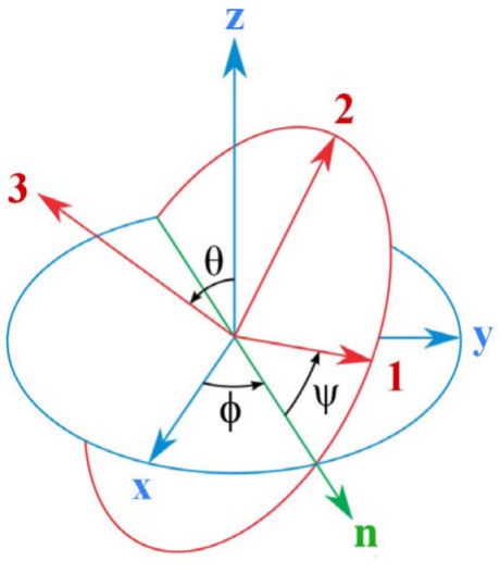
The z − x − z sequence of rotations \lambda_{\phi} , \lambda_{\theta} , \lambda_{\psi} corresponding to the Eulerian angles (\phi , \theta , \psi ). The first rotation \phi about the space-fixed \mathbf{z} axis (blue) is from the x-axis (blue) to the line of nodes \mathbf{n} (green). The second r… — Figure 13.13.1:The $z − x − z$ sequence of rotations $\lambda_{\phi} , \lambda_{\theta} , \lambda_{\psi}$ corresponding to the Eulerian angles $(\phi , \theta , \psi )$ . The first rotation $\phi$ about the space-fixed $\mathbf{z}$ axis (blue) is from the $x$ -axis (blue) to the line of nodes $\mathbf{n}$ (green). The second rotation $\theta$ about the line of nodes (green) is from the space-fixed $z$ axis (blue) to the body-fixed 3-axis (red). The third rotation $\psi$ about the body-fixed 3-axis (red) is from the line of nodes (green) to the body-fixed 1 axis (red).

As discussed in Appendix 19.4.2, the 9 component rotation matrix involves only three independent angles. There are many possible choices for these three angles. It is convenient to use the Euler angles, $\phi , \theta , \psi ,$ (also called Eulerian angles) shown in Figure 13.13.1.^[1] The Euler angles are generated by a series of three rotations that rotate from the space-fixed $(\mathbf{\hat{x}}, \mathbf{\hat{y}},\mathbf{\hat{z}})$ system to the bodyfixed $(\mathbf{\hat{1}}, \mathbf{\hat{2}}, \mathbf{\hat{3}})$ system. The rotation must be such that the space-fixed $z$ axis rotates by an angle $\theta$ to align with the body-fixed 3 axis. This can be performed by rotating through an angle $\theta$ about the $\mathbf{\hat{n}} \equiv \mathbf{\hat{z}} \times \mathbf{\hat{3}}$ direction, where $\mathbf{\hat{z}}$ and $\mathbf{\hat{3}}$ designate the unit vectors along the “ $z$ ” axes of the space and body fixed frames respectively. The unit vector $\mathbf{\hat{n}} \equiv \mathbf{\hat{z}} \times \mathbf{\hat{3}}$ is the vector normal to the plane defined by the $\mathbf{\hat{z}}$ and $\mathbf{\hat{3}}$ unit vectors and this unit vector $\mathbf{\hat{n}} = \mathbf{\hat{z}} \times \mathbf{\hat{3}}$ is called the line of nodes. The chosen convention is that the unit vector $\mathbf{\hat{n}} = \mathbf{\hat{z}} \times \mathbf{\hat{3}}$ is along the “ $x$ ” axis of an intermediate-axis frame designated by $(\mathbf{\hat{n}}, \mathbf{\hat{y}}^{\prime} ,\mathbf{\hat{z}})$ , that is, the unit vector $\mathbf{\hat{n}} = \mathbf{\hat{z}} \times \mathbf{\hat{3}}$ plus the unit vectors $\mathbf{\hat{y}}^{\prime}$ and $\mathbf{\hat{z}}$ are in the same plane as the $\mathbf{\hat{z}}$ and $\mathbf{\hat{3}}$ unit vectors. The sequence of three rotations is performed as summarized below.

1) Rotation $\phi$ about the space-fixed $\mathbf{\hat{z}}$ axis from the space $\mathbf{\hat{x}}$ axis to the line of nodes $\mathbf{\hat{n}}$ :¶

The first rotation $(\mathbf{x}, \mathbf{y}, \mathbf{z}) \cdot \boldsymbol{\lambda}_{\phi} \rightarrow (\mathbf{n}, \mathbf{y}^{\prime} , \mathbf{z})$ is in a right-handed direction through an angle $\phi$ about the space-fixed $\mathbf{z}$ axis. Since the rotation takes place in the $\mathbf{x} − \mathbf{y}$ plane, the transformation matrix is

\{\boldsymbol{\lambda}_{\phi} \} = \begin{pmatrix} \cos \phi & \sin \phi & 0 \\ − \sin \phi & \cos \phi & 0 \\ 0 & 0 & 1 \end{pmatrix}

This leads to the intermediate coordinate system $(\mathbf{n}, \mathbf{y}^{\prime} , \mathbf{z})$ where the rotated $\mathbf{x}$ axis now is colinear with the $\mathbf{n}$ axis of the intermediate frame, that is, the line of nodes.

(\mathbf{n}, \mathbf{y}^{\prime} , \mathbf{z}) = \{\boldsymbol{\lambda}_{\phi} \} \cdot (\mathbf{x}, \mathbf{y}, \mathbf{z})

The precession angular velocity $\dot{\phi}$ is the rate of change of angle of the line of nodes with respect to the space $x$ axis about the space-fixed $z$ axis.

2) Rotation $\theta$ about the line of nodes $\mathbf{\hat{n}}$ from the space $\mathbf{\hat{z}}$ axis to the body-fixed $\mathbf{\hat{3}}$ axis:¶

The second rotation

(\mathbf{n}, \mathbf{y}^{\prime} , \mathbf{z}) \cdot \lambda_{\theta} \rightarrow (\mathbf{n}, \mathbf{y}^{\prime\prime}, \mathbf{3})

is in a right-handed direction through the angle $\theta$ about the $\mathbf{\hat{n}}$ axis (line of nodes) so that the “ $z$ ” axis becomes colinear with the body-fixed $\mathbf{\hat{3}}$ axis. Because the rotation now is in the $\mathbf{\hat{z}}−\mathbf{\hat{3}}$ plane, the transformation matrix is

\{\boldsymbol{\lambda}_{\theta} \} = \begin{pmatrix} 1 & 0 & 0 \\ 0 & \cos \theta & \sin \theta \\ 0 & − \sin \theta & \ cos \theta \end{pmatrix}

The line of nodes which is at the intersection of the space-fixed and body-fixed planes, shown in Figure 13.13.1, points in the $\mathbf{\hat{n}} = \mathbf{\hat{z}} \times \mathbf{\hat{3}}$ direction. The new “ $z$ ” axis now is the body-fixed $\mathbf{\hat{3}}$ axis. The angular velocity $\dot{\theta}$ is the rate of change of angle of the body-fixed $\mathbf{\hat{3}}$ -axis relative to the space-fixed $\mathbf{\hat{z}}$ -axis about the line of nodes.

3) Rotation $\psi$ about the body-fixed $\mathbf{\hat{3}}$ axis from the line of nodes to the body-fixed $\mathbf{\hat{1}}$ axis:¶

The third rotation

(\mathbf{n}, \mathbf{y}^{\prime\prime}, \mathbf{3}) \cdot \lambda_{\psi} \rightarrow (\mathbf{\hat{1}}, \mathbf{\hat{2}}, \mathbf{\hat{3}})

is in a right-handed direction through the angle $\psi$ about the new body-fixed $\mathbf{\hat{3}}$ axis. This third rotation transforms the rotated intermediate $(\mathbf{n}, \mathbf{y}^{\prime\prime}, \mathbf{3})$ frame to final body-fixed coordinate system $(\mathbf{\hat{1}}, \mathbf{\hat{2}}, \mathbf{\hat{3}})$ . The transformation matrix is

\{\boldsymbol{\lambda}_{\psi} \} = \begin{pmatrix} \cos \psi & \sin \psi & 0 \\ − \sin\psi & \cos \psi & 0 \\ 0 & 0 & 1 \end{pmatrix}

The spin angular velocity $\dot{\psi}$ is the rate of change of the angle of the body-fixed $\mathbf{1}$ -axis with respect to the line of nodes about the body-fixed $\mathbf{3}$ axis.

The total rotation matrix $\{\boldsymbol{\lambda}\}$ is given by

\{\boldsymbol{\lambda}\} = \{\boldsymbol{\lambda}_{\psi} \} \cdot \{\boldsymbol{\lambda}_{\theta} \} \cdot \{\boldsymbol{\lambda}_{\phi} \} \tag{13.81}

Thus the complete rotation from the space-fixed $(\mathbf{x}, \mathbf{y}, \mathbf{z})$ axis system to the body-fixed $(\mathbf{1}, \mathbf{2}, \mathbf{3})$ axis system is given by

(\mathbf{1}, \mathbf{2}, \mathbf{3}) = \{\boldsymbol{\lambda}\} \cdot (\mathbf{x}, \mathbf{y}, \mathbf{z})

where $\{\boldsymbol{\lambda}\}$ is given by the triple product Equation 13.81 leading to the rotation matrix

\{\boldsymbol{\lambda}\} = \begin{pmatrix} \cos \phi \cos \psi − \sin \phi \cos \theta \sin \psi & \sin \phi \cos \psi + \cos \phi \cos \theta \sin \psi & \sin \theta \sin \psi \\ − \cos \phi \sin \psi − \sin \phi \cos \theta \cos \psi & − \sin \phi \sin \psi + \cos \phi \cos \theta \cos \psi & \sin \theta \cos \psi \\ \sin \phi \sin \theta & − \cos \phi \sin \theta & \cos \theta \end{pmatrix}

The inverse transformation from the body-fixed axis system to the space-fixed axis system is given by

(\mathbf{x}, \mathbf{y}, \mathbf{z}) = \{\boldsymbol{\lambda}\}^{− 1} \cdot (\mathbf{1}, \mathbf{2}, \mathbf{3})

where the inverse matrix $\{\boldsymbol{\lambda}\}^{−1}$ equals the transposed rotation matrix $\{\boldsymbol{\lambda}\}^{T}$ , that is,

\{\boldsymbol{\lambda}\}^{−1} = \{\boldsymbol{\lambda}\}^T = \begin{pmatrix} \cos \phi \cos \psi − \sin \phi \cos \theta \sin \psi & − \cos \phi \sin \psi − \sin \phi \cos \theta \cos \psi & \sin \phi \sin \theta \\ \sin \phi \cos \psi + \cos \phi \cos \theta \sin \psi & − \sin \phi \sin \psi + \cos \phi \cos \theta \cos \psi & - \cos \phi \sin \theta \\ \sin \theta \sin \psi & \sin \theta \cos \psi & \cos \theta \end{pmatrix}

Taking the product $\{\boldsymbol{\lambda}\} \{\boldsymbol{\lambda}\}^{ −1} = 1$ shows that the rotation matrix is a proper, orthogonal, unit matrix.

The use of three different coordinate systems, space-fixed, the intermediate line of nodes, and the body-fixed frame can be confusing at first glance. Basically the angle $\phi$ specifies the rotation about the space-fixed $z$ axis between the space-fixed $x$ axis and the line of nodes of the Euler angle intermediate frame. The angle $\psi$ specifies the rotation about the body-fixed 3 axis between the line of nodes and the body-fixed 1 axis. Note that although the space-fixed and body-fixed axes systems each are orthogonal, the Euler angle basis in general is not orthogonal. For rigid-body rotation the rotation angle $\phi$ about the space-fixed $z$ axis is time dependent, that is, the line of nodes is rotating with an angular velocity $\dot{\phi}$ with respect to the space-fixed coordinate frame. Similarly the body-fixed coordinate frame is rotating about the body-fixed 3 axis with angular velocity $\dot{\psi}$ relative to the line of nodes.

Example 13.13.1: Euler angle transformation

The definition of the Euler angles can be confusing, therefore it is useful to illustrate their use for a rotational transformation of a primed frame $(x^{\prime}, y^{\prime} , z^{\prime} )$ to an unprimed frame $(x,y,z)$ . Assume the first rotation about the $z^{\prime}$ axis, is $\phi = 30^{\circ}$

\lambda_{\phi} = \begin{pmatrix} \frac{\sqrt{3}}{2} & \frac{1}{2} & 0 \\ −\frac{1}{2} & \frac{\sqrt{3}}{2} & 0 \\ 0 & 0 & 1 \end{pmatrix} \notag

Let the second rotation be $\theta = 45^{\circ}$ about the line of nodes, that is, the intermediate $x$ ” axis. Then

\lambda_{\theta} = \begin{pmatrix} 1 & 0 & 0 \\ 0 & \frac{1}{\sqrt{2}} & \frac{1}{\sqrt{2}} \\ 0 & -\frac{1}{\sqrt{2}} & \frac{1}{\sqrt{2}} \end{pmatrix} \notag

Let the third rotation be $\psi = 90^{\circ}$ about the $z$ axis.

\lambda_{\psi} = \begin{pmatrix} 0 & 1 & 0 \\ −1 & 0 & 0 \\ 0 & 0 & 1 \end{pmatrix} \notag

Thus the net rotation corresponds to $\lambda = \lambda_{\psi} \lambda_{\theta} \lambda_{\phi}$

\lambda = \begin{pmatrix} \frac{\sqrt{3}}{2} & \frac{1}{2} & 0 \\ −\frac{1}{2} & \frac{\sqrt{3}}{2} & 0 \\ 0 & 0 & 1 \end{pmatrix} \begin{pmatrix} 1 & 0 & 0 \\ 0 & \frac{1}{\sqrt{2}} & \frac{1}{\sqrt{2}} \\ 0 & -\frac{1}{\sqrt{2}} & \frac{1}{\sqrt{2}} \end{pmatrix} \begin{pmatrix} 0 & 1 & 0 \\ −1 & 0 & 0 \\ 0 & 0 & 1 \end{pmatrix} = \begin{pmatrix} -\frac{1}{4}\sqrt{2} & \frac{1}{2}\sqrt{3} & \frac{1}{4}\sqrt{2} \\ −\frac{1}{4}\sqrt{6} & -\frac{1}{2} & \frac{1}{4}\sqrt{6} \\ \frac{1}{2}\sqrt{2} & 0 & \frac{1}{2}\sqrt{2} \end{pmatrix} \notag

13.14: Angular Velocity¶

Angular velocity $\omega$ ¶

It is useful to relate the rigid-body equations of motion in the space-fixed $(\mathbf{\hat{x}}, \mathbf{\hat{y}},\mathbf{\hat{z}})$ coordinate system to those in the body-fixed $(\mathbf{\hat{e}}_1,\mathbf{\hat{e}}_2,\mathbf{\hat{e}}_3)$ coordinate system where the principal axis inertia tensor is defined. It was shown in appendix 19.4 that an infinitessimal rotation can be represented by a vector. Thus the time derivatives of these rotation angles can be associated with the components of the angular velocity $\boldsymbol{\omega}$ , where the precession $\omega_{\phi} = \dot{\phi}$ , the nutation $\omega_{\theta} = \dot{\theta}$ , and the spin $\omega_{\psi} = \dot{\psi}$ . Unfortunately the coordinates $(\phi , \theta , \psi)$ are with respect to mixed coordinate frames and thus are not orthogonal axes. That is, the Euler angular velocities are expressed in different coordinate frames, where the precession $\dot{\phi}$ is around the space-fixed $\mathbf{\hat{z}}$ axis measured relative to the $\mathbf{\hat{x}}$ -axis, the spin $\dot{\psi}$ is around the body-fixed $\mathbf{\hat{e}}_3$ axis relative to the rotating line-of-nodes, and the nutation $\dot{\theta}$ is the angular velocity between the $\mathbf{\hat{z}}$ and $\mathbf{\hat{e}}_3$ axes and points along the instantaneous line-of-nodes in the $\mathbf{\hat{e}}_3 \times \mathbf{\hat{z}}$ direction. By reference to Figure 13.13.1 it can be seen that the components along the body-fixed axes are as given in Table 13.14.1.

Precession $\dot{\phi}$	Nutation $\dot{\theta}$	Spin $\dot{\psi}$
$\dot{\phi}_1 = \dot{\phi} \sin \theta \sin \psi$	$\dot{\theta}_1 = \dot{\theta} \cos \psi$	$\dot{\psi}_1 = 0$
$\dot{\phi}_2 = \dot{\phi} \sin \theta \cos \psi$	$\dot{\theta}_2 = -\dot{\theta} \sin \psi$	$\dot{\psi}_2 = 0$
$\dot{\phi}_3 = \dot{\phi} \cos \theta$	$\dot{\theta}_3 = 0$	$\dot{\psi}_3 = \psi$

Note that the precession angular velocity $\dot{\phi}$ is the angular velocity that the body-fixed $\mathbf{\hat{e}}_3$ and $\mathbf{\hat{z}} \times \mathbf{\hat{3}}$ axes precess around the space-fixed $\mathbf{\hat{z}}$ axis. Table 13.14.1 gives the Euler angular velocities required to calculate the components of the angular velocity $\boldsymbol{\omega}$ for the body-fixed $(\mathbf{1}, \mathbf{2}, \mathbf{3})$ axis system. Collecting the individual components of $\boldsymbol{\omega}$ , gives the components of the angular velocity of the body, relative to the space-fixed axes, in the body-fixed axis system $(1, 2, 3)$

\omega_1 = \dot{\phi}_1 + \dot{\theta}_1 + \dot{\psi}_1 = \dot{\phi} \sin \theta \sin \psi + \dot{\theta} \cos \psi \tag{13.86}

\omega_2 = \dot{\phi}_2 + \dot{\theta}_2 + \dot{\psi}_2 = \dot{\phi} \sin \theta \cos \psi - \dot{\theta} \sin \psi \tag{13.87}

\omega_3 = \dot{\phi}_3 + \dot{\theta}_3 + \dot{\psi}_3 = \dot{\phi} \cos \theta + \dot{\psi} \tag{13.88}

The angular velocity of the body about the body-fixed $\mathbf{3}$ -axis, $\omega_3$ , is the sum of the projection of the precession angular velocity of the line-of-nodes $\dot{\phi}$ with respect to the space-fixed $\mathbf{x}$ -axis, plus the angular velocity $\dot{\psi}$ of the body-fixed 3-axis with respect to the rotating line-of-nodes.

Similarly, the components of the body angular velocity $\boldsymbol{\omega}$ for the space-fixed axis system $(x,y,z)$ can be derived to be

\omega_x = \dot{\theta} \cos \phi + \dot{\psi} \sin \theta \sin \phi \tag{13.89}

\omega_y = \dot{\theta} \sin \phi - \dot{\psi} \sin \theta \cos \phi \tag{13.90}

\omega_z = \dot{\phi} + \dot{\psi} \cos \theta \tag{13.91}

Note that when $\theta = 0$ then the Euler angles are singular in that the space-fixed $z$ axis is parallel with the body-fixed 3 axis and there is no way of distinguishing between precession $\dot{\phi}$ and spin $\dot{\psi}$ , leading to $\omega_z = \omega_3 = \dot{\phi} + \dot{\psi}$ . When $\theta = \pi$ then the $z$ axis and 3 axis are antiparallel and $\omega_z = \dot{\phi} - \dot{\psi} = -\omega_3$ . The other special case is when $\cos \theta = 0$ for which the Euler angle system is orthogonal and the space-fixed $\omega_z = \dot{\phi}$ , that is, it equals the precession, while the body-fixed $\omega_3 = \dot{\psi}$ , that is, it equals the spin. When the Euler angle basis is not orthogonal then equations 13.86 - 13.88 and 13.89 - 13.91 are needed for expressing the Euler equations of motion in either the body-fixed frame or the space-fixed frame respectively.

Equations 13.86 - 13.88 for the components of the angular velocity in the body-fixed frame can be expressed in terms of the Euler angle velocities in a matrix form as

\begin{pmatrix} \omega_1 \\ \omega_2 \\ \omega_3 \end{pmatrix} = \begin{pmatrix} \sin \theta \sin \psi & \cos \psi & 0 \\ \sin \theta \cos \psi & - \sin \psi & 0 \\ \cos \theta & 0 & 1 \end{pmatrix} \cdot \begin{pmatrix} \dot{\phi} \\ \dot{\theta} \\ \dot{\psi} \end{pmatrix}

Note that the transformation matrix is not orthogonal which is to be expected since the Euler angular velocities are about axes that do not form a rectangular system of coordinates. Similarly equations 13.89 - 13.91 for the angular velocity in the space-fixed frame can be expressed in terms of the Euler angle velocities in matrix form as

\begin{pmatrix} \omega_x \\ \omega_y \\ \omega_z \end{pmatrix} = \begin{pmatrix} 0 & \cos \phi & \sin \theta \sin \phi \\ 0 & \sin \phi & \sin \theta \cos \phi \\ 1 & 0 & \cos \theta \end{pmatrix} \cdot \begin{pmatrix} \dot{\phi} \\ \dot{\theta} \\ \dot{\psi} \end{pmatrix}

13.15: Kinetic energy in terms of Euler angular velocities¶

The kinetic energy is a scalar quantity and thus is the same in both stationary and rotating frames of reference. It is much easier to evaluate the kinetic energy in the rotating Principal-axis frame since the inertia tensor is diagonal in the Principal-axis frame as given in equation $(13.12.14)$

T_{rot} = \frac{1}{2} \sum^3_i I_{ii} \omega^2_i

Using equation $(13.14.1-13.14.3)$ for the body-fixed angular velocities gives the rotational kinetic energy in terms of the Euler angular velocities and principal-frame moments of inertia to be

T_{rot}=\frac{1}{2}\left[I_{1}(\dot{\phi} \sin \theta \sin \psi+\dot{\theta} \cos \psi)^{2}+I_{2}(\dot{\phi} \sin \theta \cos \psi-\dot{\theta} \sin \psi)^{2}+I_{3}(\dot{\phi} \cos \theta+\dot{\psi})^{2}\right]

13.16: Rotational Invariants¶

The scalar properties of a rotating body, such as mass $M$ , Lagrangian $L$ , and Hamiltonian $H$ , are rotationally invariant, that is, they are the same in any body-fixed or laboratory-fixed coordinate frame. This fact also applies to scalar products of all vector observables such as angular momentum. For example the scalar product

\mathbf{L} \cdot \mathbf{L} = l^2 \notag

where $l$ is the root mean square value of the angular momentum. An example of a scalar invariant is the scalar product of the angular velocity

\boldsymbol{\omega} \cdot \boldsymbol{\omega} = \omega^2 \notag

where $\omega^2$ is the mean square angular velocity. The scalar product $\omega \cdot \omega = | \omega |^2$ can be calculated using the Euler-angle velocities for the body-fixed frame, equations $(13.14.1-13.14.3)$ , to be

\boldsymbol{\omega} \cdot \boldsymbol{\omega} = | \omega |^2 = \omega^2_1 + \omega^2_2 + \omega^2_3 = \dot{\phi}^2 + \dot{\theta}^2 + \dot{\psi}^2 + 2 \dot{\phi}\dot{\psi} \cos \theta \notag

Similarly, the scalar product can be calculated using the Euler angle velocities for the space-fixed frame using equations $(13.14.4-13.14.6)$ .

\boldsymbol{\omega} \cdot \boldsymbol{\omega} = | \omega |^2 = \omega^2_x + \omega^2_y + \omega^2_z = \dot{\phi}^2 + \dot{\theta}^2 + \dot{\psi}^2 + 2 \dot{\phi}\dot{\psi} \cos \theta \notag

This shows the obvious result that the scalar product $\omega \cdot \omega = | \omega |^2$ is invariant to rotations of the coordinate frame, that is, it is identical when evaluated in either the space-fixed, or body-fixed frames.

Note that for $\theta = 0$ , the $\hat{3}$ and $\hat{z}$ axes are parallel, and perpendicular to the $\hat{\theta}$ axis, then

| \omega |^2 = \left(\dot{\phi} + \dot{\psi} \right)^2 + \dot{\theta}^2 \notag

For the case when $\theta = 180^{\circ}$ , the $\hat{3}$ and $\hat{z}$ axes are antiparallel, and perpendicular to the $\hat{\theta}$ axis, then

| \omega |^2 = \left( \dot{\phi} − \dot{\psi} \right)^2 + \dot{\theta}^2 \notag

For the case when $\theta = 90^{\circ}$ , the $\hat{3}$ , $\hat{z}$ , and $\hat{\theta}$ axes are mutually perpendicular, that is, orthogonal, and then

| \omega |^2 = \dot{\phi}^2 + \dot{\psi}^2 + \dot{\theta}^2 \notag

The time-averaged shape of a rapidly-rotating body, as seen in the fixed inertial frame, is very different from the actual shape of the body, and this difference depends on the rotational frequency. For example, a pencil rotating rapidly about an axis perpendicular to the body-fixed symmetry axis has an average shape that is a flat disk in the laboratory frame which bears little resemblance to a pencil. The actual shape of the pencil could be determined by taking high-speed photographs which display the instantaneous body-fixed shape of the object at given times. Unfortunately for fast rotation, such as rotation of a molecule or a nucleus, it is not possible to take photographs with sufficient speed and spatial resolution to observe the instantaneous shape of the rotating body. What is measured is the average shape of the body as seen in the fixed laboratory frame. In principle the shape observed in the fixed inertial frame can be related to the shape in the body-fixed frame, but this requires knowing the body-fixed shape which in general is not known. For example, a deformed nucleus may be both vibrating and rotating about some triaxially deformed average shape which is a function of the rotational frequency. This is not apparent from the shapes measured in the fixed frame for each of the excited states.

The fact that scalar products are rotationally invariant, provides a powerful means of transforming products of observables in the body-fixed frame, to those in the laboratory frame. In 1971 Cline developed a powerful model-independent method that utilizes rotationally-invariant products of the electromagnetic quadrupole operator $E2$ to relate the electromagnetic $E2$ properties for the observed levels of a rotating nucleus measured in the laboratory frame, to the electromagnetic $E2$ properties of the deformed rotating nucleus measured in the body-fixed frame.[Cli71, Cli72, Cli86] The method uses the fact that scalar products of the electromagnetic multipole operators are rotationally invariant. This allows transforming scalar products of a complete set of measured electromagnetic matrix elements, measured in the laboratory frame, into the electromagnetic properties in the body-fixed frame of the rotating nucleus. These rotational invariants provide a model-independent determination of the magnitude, triaxiality, and vibrational amplitudes of the average shapes in the body-fixed frame for individual observed nuclear states that may be undergoing both rotation and vibration. When the bombarding energy is below the Coulomb barrier, the scattering of a projectile nucleus by a target nucleus is due purely to the electromagnetic interaction since the distance of closest approach exceeds the range of the nuclear force. For such pure Coulomb collisions, the electromagnetic excitation of collective nuclei populates many excited states with cross sections that are a direct measure of the $E2$ matrix elements. These measured matrix elements are precisely those required to evaluate, in the laboratory frame, the $E2$ rotational invariants from which it is possible to deduce the intrinsic quadrupole shapes of the rotating-vibrating nuclear states in the body-fixed frame[Cli86].

13.17: Euler’s equations of motion for rigid-body rotation¶

Rigid-body rotation can be confusing in that two coordinate frames are involved and, in general, the angular velocity and angular momentum are not aligned. The motion of the rigid body is observed in the space-fixed inertial frame whereas it is simpler to calculate the equations of motion in the body-fixed principal axis frame, for which the inertia tensor is known and is constant. The rigid body is rotating with angular velocity vector $\boldsymbol{\omega}$ , which is not aligned with the angular momentum $\mathbf{L}$ . For torque-free angular momentum, $\mathbf{L}$ is conserved and has a fixed orientation in the space-fixed axis system. Euler’s equations of motion, presented below, are given in the body-fixed frame for which the inertial tensor is known since this simplifies solution of the equations of motion. However, this solution has to be rotated back into the space-fixed frame to describe the rotational motion as seen by an observer in the inertial frame.

This chapter has introduced the inertial properties of a rigid body, as well as the Euler angles for transforming between the body-fixed and inertial frames of reference. This has prepared the stage for solving the equations of motion for rigid-body motion, namely, the dynamics of rotational motion about a body-fixed point under the action of external forces. The Euler angles are used to specify the instantaneous orientation of the rigid body.

In Newtonian mechanics, the rotational motion is governed by the equivalent Newton’s second law given in terms of the external torque $\mathbf{N}$ and angular momentum $\mathbf{L}$

\mathbf{N} = \left( \frac{d\mathbf{L}}{dt}\right)_{space}

Note that this relation is expressed in the inertial space-fixed frame of reference, not the non-inertial body-fixed frame. The subscript $space$ is added to emphasize that this equation is written in the inertial space-fixed frame of reference. However, as already discussed, it is much more convenient to transform from the space-fixed inertial frame to the body-fixed frame for which the inertia tensor of the rigid body is known. Thus the next stage is to express the rotational motion in terms of the body-fixed frame of reference. For simplicity, translational motion will be ignored.

The rate of change of angular momentum can be written in terms of the body-fixed value, using the transformation from the space-fixed inertial frame $(\mathbf{\hat{x}}, \mathbf{\hat{y}},\mathbf{\hat{z}})$ to the rotating frame $(\mathbf{\hat{e}}_1,\mathbf{\hat{e}}_2,\mathbf{\hat{e}}_3)$ as given in chapter 13.13,

\mathbf{N} = \left( \frac{d\mathbf{L}}{dt}\right)_{space} = \left( \frac{d\mathbf{L}}{dt}\right)_{body} + \boldsymbol{\omega} \times \mathbf{L}

However, the body axis $\mathbf{\hat{e}}_i$ is chosen to be the principal axis such that

L_i = I_i \omega_i

where the principal moments of inertia are written as $I_i$ . Thus the equation of motion can be written using the body-fixed coordinate system as

\begin{align} \mathbf{N} & = I_1 \dot{\omega}_1\mathbf{\hat{e}}_1 + I_2 \dot{\omega}_2\mathbf{\hat{e}}_2 + I_3 \dot{\omega}_3 \mathbf{\hat{e}}_3 + \begin{vmatrix} \mathbf{\hat{e}}_1 & \mathbf{\hat{e}}_2 & \mathbf{\hat{e}}_3 \\ \omega_1 & \omega_2 & \omega_3 \\ I_1\omega_1 & I_2\omega_2 & I_3\omega_3 \end{vmatrix} \\ & = (I_1 \dot{\omega}_1 − (I_2 − I_3) \omega_2\omega_3) \mathbf{\hat{e}}_1 + (I_2 \dot{\omega}_2 − (I_3 − I_1) \omega_3\omega_1)\mathbf{\hat{e}}_2 + (I_3 \dot{\omega}_3 − (I_1 − I_2) \omega_1\omega_2)\mathbf{\hat{e}}_3 \end{align}

where the components in the body-fixed axes are given by

\begin{align} N_1 = I_1 \dot{\omega}_1 − (I_2 − I_3) \omega_2\omega_3 \\ N_2 = I_2 \dot{\omega}_2 − (I_3 − I_1) \omega_3\omega_1 \notag \\ N_3 = I_3 \dot{\omega}_3 − (I_1 − I_2) \omega_1\omega_2 \notag \end{align}

These are the Euler equations for rigid body in a force field expressed in the body-fixed coordinate frame. They are applicable for any applied external torque $\mathbf{N}$ .

The motion of a rigid body depends on the structure of the body only via the three principal moments of inertia $I_1$ , $I_2$ , and $I_3$ . Thus all bodies having the same principal moments of inertia will behave exactly the same even though the bodies may have very different shapes. As discussed earlier, the simplest geometrical shape of a body having three different principal moments is a homogeneous ellipsoid. Thus, the rigid-body motion often is described in terms of the equivalent ellipsoid that has the same principal moments.

A deficiency of Euler’s equations is that the solutions yield the time variation of $\boldsymbol{\omega}$ as seen from the body-fixed reference frame axes, and not in the observers fixed inertial coordinate frame. Similarly the components of the external torques in the Euler equations are given with respect to the body-fixed axis system which implies that the orientation of the body is already known. Thus for non-zero external torques the problem cannot be solved until the orientation is known in order to determine the components $N^{ext}_i$ . However, these difficulties disappear when the external torques are zero, or if the motion of the body is known and it is required to compute the applied torques necessary to produce such motion.

13.18: Lagrange equations of motion for rigid-body rotation¶

The Euler equations of motion were derived using Newtonian concepts of torque and angular momentum. It is of interest to derive the equations of motion using Lagrangian mechanics. It is convenient to use a generalized torque $N$ and assume that $U = 0$ in the Lagrange-Euler equations. Note that the generalized force is a torque since the corresponding generalized coordinate is an angle, and the conjugate momentum is angular momentum. If the body-fixed frame of reference is chosen to be the principal axes system, then, since the inertia tensor is diagonal in the principal axis frame, the kinetic energy is given in terms of the principal moments of inertia as

T = \frac{1}{2} \sum_i I_i \omega^2_i \tag{13.104}

Using the Euler angles as generalized coordinates, then the Lagrange equation for the specific case of the $\psi$ coordinate and including a generalized force $N_{\psi}$ gives

\frac{d}{dt} \frac{\partial T}{\partial \dot{\psi}} − \frac{\partial T}{\partial \psi} = N_{\psi}

which can be expressed as

\frac{d}{dt} \sum^3_i \frac{\partial T}{\partial \omega_i} \frac{\partial \omega_i}{\partial \dot{\psi}} − \sum^3_i \frac{\partial T}{\partial \omega_i} \frac{\partial \omega_i}{\partial \psi } = N_{\psi} \tag{13.106}

Equation 13.104 gives

\frac{\partial T}{\partial \omega_i} = I_i \omega_i

Differentiating the angular velocity components in the body-fixed frame, equations $(13.14.1-13.14.3)$ give

$\frac{\partial \omega_1}{\partial \psi} = \dot{\phi} \sin \theta \cos \psi − \dot{\theta} \sin\psi = \omega_2$	$\frac{\partial \omega_1 }{\partial \dot{\psi}} = \frac{\partial \omega_2}{ \partial \dot{\psi}} = 0$
$\frac{\partial \omega_2 }{\partial \psi} = −\dot{\phi} \sin \theta \sin \psi − \dot{\theta} \cos \psi = −\omega_1$	$\frac{\partial \omega_1 }{\partial \dot{\psi}} = \frac{\partial \omega_2}{ \partial \dot{\psi}} = 0$
$\frac{\partial \omega_3}{\partial \psi} = 0$	$\frac{\partial \omega_3 }{\partial \dot{\psi}} = 1$

Substituting these into the Lagrange Equation 13.106 gives

\frac{d}{dt} I_3\omega_3 − I_1\omega_1\omega_2 + I_2\omega_2 (−\omega_1) = N_3

since the $\psi$ and $\widehat{\mathbf{e}_3}$ axes are colinear. This can be rewritten as

I_3\dot{\omega}_3 − (I_1 − I_2) \omega_1\omega_2 = N_3

Any axis could have been designated the $\widehat{\mathbf{e}_3}$ axis, thus the above equation can be generalized to all three axes to give

\begin{align} I_1\dot{\omega}_1 − (I_2 − I_3) \omega_2\omega_3 = N_1 \\ I_2\dot{\omega}_2 − (I_3 − I_1) \omega_3\omega_1 = N_2 \notag \\ I_3\dot{\omega}_3 − (I_1 − I_2) \omega_1\omega_2 = N_3 \notag \end{align}

These are the Euler’s equations given previously in $(13.17.6)$ . Note that although $\dot{\omega}_3$ is the equation of motion for the $\psi$ coordinate, this is not true for the $\boldsymbol{\phi}$ and $\boldsymbol{\theta}$ rotations which are not along the body-fixed $x_1$ and $x_2$ axes as given in table 13.14.1.

Example 13.18.1: Rotation of a dumbbell

Figure 13.18.1:Rotation of a dumbbell.

Consider the motion of the symmetric dumbbell shown in the adjacent figure. Let $|r_1| = |r_2| = b$ . Let the body-fixed coordinate system have its origin at $O$ and symmetry axis $\widehat{\mathbf{e}_3}$ be along the weightless shaft toward $m_1$ and $\mathbf{v}_{\alpha} = v_{\alpha} \hat{e}_1$ . The angular momentum is given by

\mathbf{L} = \sum_i m_i \mathbf{r} \times \mathbf{v}\notag

Because $\mathbf{L}$ is perpendicular to the shaft, and $\mathbf{L}$ rotates around $\boldsymbol{\omega}$ as the shaft rotates, let $\widehat{\mathbf{e}_2}$ be along $\mathbf{L}$ .

\mathbf{L} = L_2 \widehat{\mathbf{e}_2} \notag

If $\alpha$ is the angle between $\boldsymbol{\omega}$ and the shaft, the components of $\boldsymbol{\omega}$ are

\begin{aligned} \omega_1 = 0 \\ \omega_2 = \omega \sin \alpha \\ \omega_3 = \omega \cos \alpha \end{aligned}

Assume that the principal moments of the dumbbell are

\begin{aligned} I_1 = (m_1 + m_2) b^2 \\ I_2 = (m_1 + m_2) b^2 \\ I_3 = 0 \end{aligned}

Thus the angular momentum is given by

\begin{aligned} L_1 = I_1\omega_1 = 0 \\ L_2 = I_2\omega_2 = (m_1 + m_2) b^2 \omega \sin \alpha \\ L_3 = I_3 \omega_3 = 0 \end{aligned}

which is consistent with the angular momentum being along the $\widehat{\mathbf{e}_2}$ axis.

Using Euler’s equations, and assuming that the angular velocity is constant, i.e. $\dot{\omega}= 0$ , then the components of the torque required to satisfy this motion are

\begin{aligned} N_1 = − (m_1 + m_2) b^2 \omega^2 \sin \alpha \cos \alpha \\ N_2 = 0 \\ N_3 = 0 \end{aligned}

That is, this motion can only occur in the presence of the above applied torque which is in the direction $-\widehat{\mathbf{e}_1}$ , that is, mutually perpendicular to $\widehat{\mathbf{e}_2}$ and $\widehat{\mathbf{e}_3}$ . This torque can be written as $\mathbf{N} = \boldsymbol{\omega} \times \mathbf{L}$ .

13.19: Hamiltonian equations of motion for rigid-body rotation¶

The Hamiltonian equations of motion are expressed in terms of the Euler angles plus their corresponding canonical angular momenta $(\phi , \theta , \psi , p_{\phi} , p_{ \theta }, p_{\psi} )$ in contrast to Lagrangian mechanics which is based on the Euler angles plus their corresponding angular velocities $(\phi , \theta , \psi , \dot{\phi} , \dot{\theta} , \dot{\psi})$ . The Hamiltonian approach is conveniently expressed in terms of a set of Andoyer-Deprit action-angle coordinates that include the three Euler angles, specifying the orientation of the body-fixed frame, plus the corresponding three angles specifying the orientation of the spin frame of reference. This phase space approach[Dep67] can be employed for calculations of rotational motion in celestial mechanics that can include spin-orbit coupling. This Hamiltonian approach is beyond the scope of the present textbook.

13.20: Torque-free rotation of an inertially-symmetric rigid rotor¶

Euler’s equations of motion¶

There are many situations where one has rigid-body motion free of external torques, that is, $\mathbf{N} = 0$ . The tumbling motion of a jugglers baton, a diver, a rotating galaxy, or a frisbee, are examples of rigid-body rotation. For torque-free rotation, the body will rotate about the center of mass, and thus the inertia tensor with respect to the center of mass is required. An inertially-symmetric rigid body has two identical principal moments of inertia with $I_1 = I_2 \neq I_3$ , and provides a simple example that illustrates the underlying motion. The force-free Euler equations for the symmetric body in the body-fixed principal axis system are given by

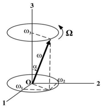
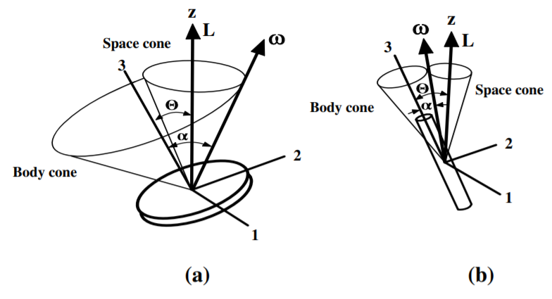
\begin{align} (I_2 − I_3) \omega_2\omega_3 − I_1\dot{\omega}_1 &= 0 \tag{13.111} \\[4pt] (I_3 − I_1) \omega_3\omega_1 − I_2\dot{\omega}_2 &= 0 \tag{13.112} \\[4pt] I_3\dot{\omega}_3 &= 0 \tag{13.113} \end{align}

where $I_1 = I_2$ and $N = 0$ apply.

The force-free symmetric top angular velocity \omega precesses on a conical trajectory about the body-fixed symmetry axis \mathbf{\hat{3}}. — Figure 13.20.1:The force-free symmetric top angular velocity $\omega$ precesses on a conical trajectory about the body-fixed symmetry axis $\mathbf{\hat{3}}$ .

Note that for torque-free motion of an inertially symmetric body Equation 13.113 implies that $\dot{\omega}_3 = 0$ , i.e. $\omega_3$ is a constant of motion and thus is a cyclic variable for the symmetric rigid body.

Equations 13.111 and 13.112 can be written as two coupled equations

\dot{\omega}_1 + \Omega \omega_2 = 0 \tag{13.114}

\dot{\omega}_2 − \Omega \omega_1 = 0 \tag{13.115}

where the precession angular velocity $\mathbf{\Omega} = \dot{\psi}$ with respect to the body-fixed frame is defined to be

\mathbf{\Omega} \equiv \left( \frac{(I_3 − I_1)}{I_1} \boldsymbol{\omega}_3 \right) \tag{13.116}

Combining the time derivatives of equations 13.114 and 13.115 leads to two uncoupled equations

\ddot{\omega}_1 + \Omega^2 \omega_1 = 0

\ddot{\omega}_2 + \Omega^2 \omega_2 = 0

These are the differential equations for a harmonic oscillator with solutions

\omega_1 = A \cos \Omega t

\omega_2 = A \sin \Omega t

These equations describe a vector $A$ rotating in a circle of radius $A$ about an axis perpendicular to $\hat{e}_3$ , that is, rotating in the $\hat{e}_1 − \hat{e}_2$ plane with angular frequency $\Omega = −\dot{\psi}$ . Note that

\omega^2_1 + \omega^2_2 = A^2 \tag{13.120}

which is a constant. In addition $\omega_3$ is constant, therefore the magnitude of the total angular velocity

|\boldsymbol{\omega} | = \sqrt{ \omega^2_1 + \omega^2_2 + \omega^2_3 }= \text{ constant} \tag{13.121}

The motion of the torque-free symmetric body is that the angular velocity $\boldsymbol{\omega}$ precesses around the symmetry axis $\hat{e}_3$ of the body at an angle $\alpha$ with a constant precession frequency $\Omega$ with respect to the body-fixed frame as shown in Figure 13.20.1. Thus, to an observer on the body, $\boldsymbol{\omega}$ traces out a cone around the body-fixed symmetry axis. Note from 13.116 that the vectors $\Omega \hat{e}_3$ and $\omega_3\hat{e}_3$ are parallel when $\Omega$ is positive, that is, $I_3 > I$ (oblate shape) and antiparallel if $I_3 < I$ (prolate shape).

For the system considered, the orientation of the angular momentum vector $\mathbf{L}$ must be stationary in the space-fixed inertial frame since the system is torque free, that is, $\mathbf{L}$ is a constant of motion. Also we have that the projection of the angular momentum on the body-fixed symmetry axis is a constant of motion, that is, it is a cyclic variable. Thus

L_3 = I_3 \omega_3 = \frac{I_1I_3}{(I_3 − I_1)} \Omega

Understanding the relation between the angular momentum and angular velocity is facilitated by considering another constant of motion for the torque-free symmetric rotor, namely the rotational kinetic energy.

T_{rot} = \frac{1}{2} \boldsymbol{\omega} \cdot \mathbf{L} = \text{ constant}

Since $\mathbf{L}$ is a constant for torque-free motion, and also the magnitude of $\boldsymbol{\omega}$ was shown to be constant, therefore the angle between these two vectors must be a constant to ensure that also $T_{\mathbf{rot}} = \frac{1}{2}\boldsymbol{\omega} \cdot \mathbf{L} =$ constant. That is, $\mathbf{\omega}$ precesses around $\mathbf{L}$ at a constant angle $(\theta − \alpha )$ such that the projection of $\boldsymbol{\omega}$ onto $\mathbf{L}$ is constant. Note that

\boldsymbol{\omega} \times \widehat{\mathbf{e}_3} = \omega_2 \widehat{\mathbf{e}_1} − \omega_1\widehat{\mathbf{e}_2}

and, for a symmetric rotor,

\mathbf{L} \cdot \boldsymbol{\omega} \times \widehat{\mathbf{e}_3} = I_1\omega_1\omega_2 − I_2\omega_1\omega_2 = 0

since $I_1 = I_2$ for the symmetric rotor. Because $\mathbf{L} \cdot \boldsymbol{\omega} \times \widehat{\mathbf{e}_3} = 0$ for a symmetric top then $\mathbf{L}$ , $\boldsymbol{\omega}$ and $\widehat{\mathbf{e}_3}$ are coplanar.

Figure 13.20.2 shows the geometry of the motion for both oblate and prolate axially-deformed bodies. To an observer in the space-fixed inertial frame, the angular velocity $\boldsymbol{\omega}$ traces out a cone that precesses with angular velocity $\Omega$ around the space fixed $\mathbf{L}$ axis called the space cone. For convenience, Figure 13.20.2 assumes that $\mathbf{L}$ and the space-fixed inertial frame $\hat{\mathbf{z}}$ axis are colinear. The angular velocity $\boldsymbol{\omega}$ also traces out the body cone as it precesses about the body-fixed $\hat{\mathbf{e}}_3$ axis. Since $\mathbf{L}$ , $\boldsymbol{\omega}$ and $\widehat{\mathbf{e}_3}$ are coplanar, then the $\boldsymbol{\omega}$ vector is at the intersection of the space and body cones as the body cone rolls around the space cone. That is, the space and body cones have one generatrix in common which coincides with $\boldsymbol{\omega}$ . As shown in Figure 13.20.2b, for a needle the body cone appears to roll without slipping on the outside of the space cone at the precessional velocity of $\Omega = −\omega$ . By contrast, as shown in Figure 13.20.2a for an oblate (disc-shaped) symmetric top the space cone rolls inside the body cone and the precession $\Omega$ is faster than $\omega$ .

Since no external torques are acting for torque-free motion, then the magnitude and direction of the total angular momentum are conserved. The description of the motion is simplified if $\mathbf{L}$ is taken to be along the space-fixed $\hat{\mathbf{z}}$ axis, then the Euler angle $\theta$ is the angle between the body-fixed basis vector $\hat{\mathbf{e}}_3$ and space-fixed basis vector $\hat{\mathbf{z}}$ . If at some instant in the body frame, it is assumed that $\widehat{\mathbf{e}_2}$ is aligned in the plane of $\mathbf{L}$ , $\boldsymbol{\omega}$ and $\widehat{\mathbf{e}_3}$ , then

L_1 = 0 \quad L_2 = L \sin \theta \quad L_3 = L\cos \theta \tag{13.126}

If $\alpha$ is the angle between the angular velocity $\boldsymbol{\omega}$ and the body-fixed $\hat{\mathbf{e}}_3$ axis, then at the same instant

\omega_1 = 0 \quad \omega_2 = \omega \sin \alpha \quad \omega_3 = \omega \cos \alpha \tag{12.127}

Torque-free rotation of symmetric tops; (a) circular flat disk, (b) circular rod. The space-fixed and body-fixed cones are shown by fine lines. The space-fixed axis system is designated by the unit vectors (\hat{\mathbf{x}}, \hat{\mathbf{y}},\hat{\mathbf{z}}) and the body-fixed principal axis sys… — Figure 13.20.2:Torque-free rotation of symmetric tops; (a) circular flat disk, (b) circular rod. The space-fixed and body-fixed cones are shown by fine lines. The space-fixed axis system is designated by the unit vectors $(\hat{\mathbf{x}}, \hat{\mathbf{y}},\hat{\mathbf{z}})$ and the body-fixed principal axis system by unit vectors $(\hat{\mathbf{1}}, \hat{\mathbf{2}}, \hat{\mathbf{3}})$ .

The components of the angular momentum also can be derived from $\mathbf{L} = \mathbf{I} \cdot \boldsymbol{\omega}$ to give

L_1 = I_1\omega_1 = 0 \quad L_2 = I_2 \omega_2 = I_1\omega \sin \alpha \quad L_3 = I_3\omega_3 = I_3\omega \cos \alpha \tag{13.128}

Equations 13.126 and 13.128 give two relations for the ratio $\frac{L_2}{L_3}$ , that is,

\frac{L_2}{L_3} = \tan \theta = \frac{I_1}{I_3} \tan \alpha \tag{13.129}

For a prolate spheroid $I_1 > I_3$ therefore $\theta > \alpha$ while $\Omega$ and $\omega_3$ have opposite signs.

For a oblate spheroid $I_1 < I_3$ therefore $\alpha > \theta$ while $\Omega$ and $\omega_3$ have the same sign.

The sense of precession can be understood if the body cone rolls without slipping on the outside of the space cone with $\Omega$ in the opposite orientation to $\omega$ for the prolate case, while for the oblate case the space cone rolls inside the body cone with $\Omega$ and $\omega$ oriented in similar directions. Note from 13.129 that $\theta = 0$ if $\alpha = 0$ , that is $\mathbf{L}$ , $\boldsymbol{\omega}$ and the $\mathbf{3}$ axis are aligned corresponding to a principal axis. Similarly, $\theta = 90^{\circ}$ if $\alpha = 90^{\circ}$ , then again $\mathbf{L}$ and $\boldsymbol{\omega}$ are aligned corresponding to them being principal axes.

Lagrangian mechanics has been used to calculate the motion with respect to the body-fixed principal axis system. However, the motion needs to be known relative to the space-fixed inertial frame where the motion is observed. This transformation can be done using the following relation

\left(\frac{d \hat{\mathbf{e}}_3}{dt}\right)_{space} = \left(\frac{d\hat{\mathbf{e}}_3}{dt} \right)_{body} + \boldsymbol{\omega} \times \hat{\mathbf{e}}_3 = \boldsymbol{\omega} \times \hat{\mathbf{e}}_3

since the unit vector $\hat{\mathbf{e}}_3$ is stationary in the body-fixed frame. The vector product of $\boldsymbol{\omega} \times \hat{\mathbf{e}}_3$ and $\hat{\mathbf{e}}_3$ gives

\begin{align*} \hat{\mathbf{e}}_3 \times \left(\frac{d\hat{\mathbf{e}}_3}{dt}\right)_{space} &= \hat{\mathbf{e}}_3 \times \boldsymbol{\omega} \times \hat{\mathbf{e}}_3 \\[4pt] &= (\hat{\mathbf{e}}_3 \cdot \hat{\mathbf{e}}_3) \boldsymbol{\omega} − (\hat{\mathbf{e}}_3 \cdot \boldsymbol{\omega} ) \hat{\mathbf{e}}_3 = \boldsymbol{\omega} − \omega_3 \hat{\mathbf{e}}_3 \end{align*}

therefore

\boldsymbol{\omega} = \hat{\mathbf{e}}_3 \times \left(\frac{d\hat{\mathbf{e}}_3}{dt}\right)_{space} + \omega_3\hat{\mathbf{e}}_3 \tag{13.131}

The angular momentum equals $\mathbf{L} = \{\mathbf{I}\} \cdot \boldsymbol{\omega}$ . Since $\hat{\mathbf{e}}_3 \times \left(\frac{d\hat{\mathbf{e}}_3}{dt}\right)_{space}$ is perpendicular to the $\hat{\mathbf{e}}_3$ axis, then for the case with $I_1 = I_2$ ,

\mathbf{L} =I_1\hat{\mathbf{e}}_3 \times \left(\frac{d\hat{\mathbf{e}}_3}{dt}\right)_{space} + I_3\omega_3\hat{\mathbf{e}}_3 \tag{13.132}

Thus the angular momentum for a torque-free symmetric rigid rotor comprises two components, one being the perpendicular component that precesses around $\hat{\mathbf{e}}_3$ , and the other is $L_3$ .

In the space-fixed frame assume that the $\hat{\mathbf{z}}$ axis is colinear with $\mathbf{L}$ . Then taking the scalar product of $\hat{\mathbf{e}}_3$ and $\mathbf{L}$ , using Equation 13.126 gives

\begin{align} L_3 &= \hat{\mathbf{e}}_3 \cdot \mathbf{L} \\[4pt] &=I_1\hat{\mathbf{e}}_3 \cdot \hat{\mathbf{e}}_3 \times \left(\frac{d\hat{\mathbf{e}}_3}{dt}\right)_{space} + I_3\omega_3\hat{\mathbf{e}}_3 \cdot \hat{\mathbf{e}}_3 \tag{13.133} \end{align}

The first term on the right is zero and thus Equation 13.133 and 13.126 give

L_3 = I_3\omega_3 = L \cos \theta

The time dependence of the rotation of the body-fixed symmetry axis with respect to the space-fixed axis system can be obtained by taking the vector product $\hat{\mathbf{e}}_3 \times \mathbf{L}$ using Equation 13.132 and using equation $B.24$ to expand the triple vector product,

\begin{align} \hat{\mathbf{e}}_3 \times \mathbf{L} &= I_1\hat{\mathbf{e}}_3 \times \left( \hat{\mathbf{e}}_3 \times \left(\frac{d\hat{\mathbf{e}}_3}{dt}\right)_{space}\right) + I_3\omega_3\hat{\mathbf{e}}_3 \times \hat{\mathbf{e}}_3 \tag{13.135} \\[4pt] \notag &= I_1 \left[\left( \hat{\mathbf{e}}_3 \cdot \left(\frac{d\hat{\mathbf{e}}_3}{dt}\right)_{space} \right) \hat{\mathbf{e}}_3 − (\hat{\mathbf{e}}_3 \cdot \hat{\mathbf{e}}_3) \left(\frac{d\hat{\mathbf{e}}_3}{dt}\right)_{space}\right] + 0 \end{align}

since $(\hat{\mathbf{e}}_3 \times \hat{\mathbf{e}}_3)=0$ . Moreover $(\hat{\mathbf{e}}_3 \cdot \hat{\mathbf{e}}_3)=1$ , and $\hat{\mathbf{e}}_3 \cdot \left(\frac{d\hat{\mathbf{e}}_3}{dt}\right)_{space}= 0$ , since they are perpendicular, then

\left(\frac{d\hat{\mathbf{e}}_3}{dt}\right)_{space} = \frac{\mathbf{L}}{I_1} \times \hat{\mathbf{e}}_3 \tag{13.136}

This equation shows that the body-fixed symmetry axis $\hat{\mathbf{e}}_3$ precesses around the $\mathbf{L}$ , where $\mathbf{L}$ is a constant of motion for torque-free rotation. The true rotational angular velocity $\boldsymbol{\omega}$ in the space-fixed frame, given by equations 13.131, can be evaluated using Equation 13.136. Remembering that it was assumed that $\mathbf{L}$ is in the $\hat{\mathbf{z}}$ direction, that is, $\mathbf{L} =L\hat{\mathbf{z}}$ , then

\begin{align} \notag \boldsymbol{\omega} &= \hat{\mathbf{e}}_3 \times \left(\frac{d\hat{\mathbf{e}}_3}{dt}\right)_{space} + \omega_3\hat{\mathbf{e}}_3 \\[4pt] \notag &= \frac{L}{I_1} \hat{\mathbf{e}}_3 \times (\hat{\mathbf{z}} \times \hat{\mathbf{e}}_3) + \left( \frac{L \cos \alpha}{ I_3} \right) \hat{\mathbf{e}}_3 \\[4pt] &= \frac{L}{ I_1} \hat{\mathbf{z}} + L \cos \alpha \left( \frac{I_1 − I_3}{ I_1I_3}\right) \hat{\mathbf{e}}_3 \end{align}

That is, the symmetry axis of the axially-symmetric rigid rotor makes an angle $\theta$ to the angular momentum vector $L\hat{\mathbf{z}}$ and precesses around $L\hat{\mathbf{z}}$ with a constant angular velocity $\frac{L}{I_1}$ while the axial spin of the rigid body has a constant value $\frac{L}{I_3}$ . Thus, in the precessing frame, the rigid body appears to rotate about its fixed symmetry axis with a constant angular velocity $\frac{L \cos \alpha}{I_3} − \frac{L \cos \alpha}{I_1} = L \cos \alpha \left(\frac{I_1−I_3}{I_1 I_3}\right)$ . The precession of the symmetry axis looks like a wobble superimposed on the spinning motion about the body-fixed symmetry axis. The angular precession rate in the space-fixed frame can be deduced by using the fact that

\dot{\phi} \sin \theta = \omega \sin \alpha \tag{13.138}

Then using Equation 13.129 allows Equation 13.138 to be written as

\dot{\phi} = \omega \sqrt{\left[ 1 + \left(\left(\frac{I_3}{I_1}\right)^2 -1 \right) \cos^2 \alpha \right] }

which gives the precession rate about the space-fixed axis in terms of the angular velocity $\omega$ . Note that the precession rate $\dot{\phi} > \omega$ if $\frac{I_3}{I_1} > 1$ , that is, for oblate shapes, and $\dot{\phi} < \omega$ if $\frac{I_3}{I_1} < 1$ , that is, for prolate shapes.

Lagrange equations of motion¶

It is interesting to compare the equations of motion for torque-free rotation of an inertially-symmetric rigid rotor derived using Lagrange mechanics with that derived previously using Euler’s equations based on Newtonian mechanics. Assume that the principal moments about the fixed point of the symmetric top are $I_1 = I_2 \neq I_3$ and that the kinetic energy equals the rotational kinetic energy, that is, it is assumed that the translational kinetic energy $T_{trans} = 0$ . Then the kinetic energy is given by

T =\frac{1}{2} \sum_i I_i \omega^2_i =\frac{1}{2}I_1 ( \omega^2_1 + \omega^2_2 ) +\frac{1}{2}I_3\omega^2_3

Equations $(13.14.1-13.14.3)$ for the body-fixed frame give

\omega^2_1 = \left( \dot{\phi} \sin \theta \sin\psi + \dot{\theta} \cos \psi \right)^2 = \dot{\phi}^2 \sin^2 \theta \sin^2 \psi + 2 \phi \dot{\theta} \sin \theta \sin\psi \cos \psi + \dot{\theta}^2 \cos^2 \psi

\omega^2_2 = \left( \dot{\phi} \sin \theta \cos \psi − \dot{\theta} \sin\psi \right)^2 = \dot{\phi}^2 \sin^2 \theta \cos^2 \psi − 2\phi \dot{\theta} \sin \theta \sin\psi \cos \psi + \dot{\theta}^2 \sin^2 \psi

Therefore

\omega^2_1 + \omega^2_2 = \dot{\phi}^2 \sin^2 \theta + \dot{\theta}^2

and

\omega^2_3 = \left( \dot{\phi} \cos \theta + \dot{\psi} \right)^2

Therefore the kinetic energy is

T =\frac{1}{2}I_1 \left( \dot{\phi}^2 \sin^2 \theta + \dot{\theta}^2\right) +\frac{1}{2}I_3 \left( \dot{\phi} \cos \theta + \dot{\psi} \right)^2

Since the system is torque free, the scalar potential energy $U$ can be assumed to be zero, and then the Lagrangian equals

L =\frac{1}{2}I_1 \left( \dot{\phi}^2 \sin^2 \theta + \dot{\theta}^2\right) +\frac{1}{2}I_3 \left( \dot{\phi} \cos \theta + \dot{\psi} \right)^2

The angular momentum about the space-fixed $z$ axis $p_{\phi}$ is conjugate to $\phi$ . From Lagrange’s equations

\dot{p}_{\phi} = \frac{\partial L}{ \partial \phi } = 0

that is, the angular momentum about the space-fixed $z$ axis, $p_{\phi}$ is a constant of motion given by

p_{\phi} = \frac{\partial L}{ \partial \dot{\phi}} = ( I_1 \sin^2 \theta + I_3 \cos^2 \theta ) \dot{\phi} + I_3\dot{\psi} \cos \theta = \text{ constant.}

Similarly, the angular momentum about the body-fixed 3 axis is conjugate to $\psi$ . From Lagrange’s equations

\dot{p}_{\psi} = \frac{\partial L}{\partial \psi } = 0

that is, $p_{\psi}$ is a constant of motion given by

p_{\psi} = \frac{\partial L}{ \partial \dot{\psi}} = I_3 \left( \dot{\dot{\phi}} \cos \theta + \dot{\psi} \right) = I_3\omega_3 = \text{ constant}

The above two relations derived from the Lagrangian can be solved to give the precession angular velocity $\dot{\phi}$ about the space-fixed $\hat{\mathbf{z}}$ axis

\dot{\phi} = \frac{p_{\phi} − p_{\psi} \cos \theta}{I_1 \sin^2 \theta}

and the spin about the body-fixed $\mathbf{\hat{3}}$ axis $\dot{\psi}$ which is given by

\dot{\psi} = \frac{p_{\psi}}{I_3} − \frac{(p_{\phi} − p_{\psi} \cos \theta ) \cos \theta}{ I_1 \sin^2 \theta}

Since $p_{\phi}$ and $p_{\psi}$ are constants of motion, then the precessional angular velocity $\dot{\phi}$ about the space-fixed $\hat{\mathbf{z}}$ axis, and the spin angular velocity $\dot{\psi}$ , which is the spin frequency about the body-fixed $\mathbf{\hat{3}}$ axis, are constants that depend directly on $I_1$ , $I_3$ . and $\theta$ .

There is one additional constant of motion available if no dissipative forces act on the system, that is, energy conservation which implies that the total energy

E =\frac{1}{2}I_1 \left( \dot{\phi}^2 \sin^2 \theta + \dot{\theta}^2 \right) +\frac{1}{2}I_3 \left( \dot{\phi} \cos \theta + \dot{\psi} \right)^2

will be a constant of motion. But the second term on the right-hand side also is a constant of motion since $p_{\psi}$ and $I_3$ both are constants, that is

\frac{1}{2} I_3\omega^2_3 =\frac{1}{2}I_3 \left( \dot{\phi} \cos \theta + \dot{\psi} \right)^2 = \frac{p^2_{\psi}}{I_3 } = \text{ constant}

Thus energy conservation implies that the first term on the right-hand side also must be a constant given by

\frac{1}{2} I_1 ( \omega^2_1 + \omega^2_2 ) =\frac{1}{2}I_1 \left( \dot{\phi}^2 \sin^2 \theta + \dot{\theta}^2 \right) = E - \frac{p^2_{\psi}}{I_3 } = \text{ constant }

These results are identical to those given in equations 13.120 and 13.121 which were derived using Euler’s equations. These results illustrate that the underlying physics of the torque-free rigid rotor is more easily extracted using Lagrangian mechanics rather than using the Euler-angle approach of Newtonian mechanics.

Example 13.20.1: Precession rate for torque-free rotating symmetric rigid rotor

Table 13.20.1 lists the precession and spin angular velocities, in the space-fixed frame, for torque-free rotation of three extreme symmetric-top geometries spinning with constant angular momentum $\omega$ when the motion is slightly perturbed such that $\omega$ is at a small angle $\alpha$ to the symmetry axis. Note that this assumes the perpendicular axis theorem, equation $(13.9.1)$ which states that for a thin laminae $I_1 + I_2 = I_3$ giving, for a thin circular disk, $I_1 = I_2$ and thus $I_3 = 2I_1$ .

Rigid-body symmetric shape	Principal moment ratio $\frac{I_3}{I_1}$	Precession rate $\dot{\phi}$	Spin rate $\dot{\psi}$
Symmetric needle	0	0	$\omega$
Sphere	1	$\omega$	0
Thin circular disk	2	$2\omega$	$-\omega$

The precession angular velocity in the space frame ranges between 0 to $2\omega$ depending on whether the body-fixed spin angular velocity is aligned or anti-aligned with the rotational frequency $\omega$ . For an extreme prolate spheroid $\frac{I_3}{I_1} = 0$ , the body-fixed spin angular velocity $\Omega = −\omega_3$ which cancels the angular velocity $\omega$ of the rotating frame resulting in a zero precession angular velocity of the body-fixed $\hat{\mathbf{e}}_3$ axis around the space-fixed frame. The spin $\Omega = 0$ in the body-fixed frame for the rigid sphere $\frac{I_3}{I_1} = 1$ , and thus the precession rate of the body-fixed $\hat{e}_3$ axis of the sphere around the space-fixed frame equals $\omega$ . For oblate spheroids and thin disks, such as a frisbee, $\frac{I_3}{I_1} = 2$ making the body-fixed precession angular velocity $\Omega = +\omega$ which adds to the angular velocity $\omega$ and increases the precession rate up to $2\omega$ as seen in the space-fixed frame. This illustrates that the spin angular velocity can add constructively or destructively with the angular velocity $\omega$ .^[2]

13.21: Torque-free rotation of an asymmetric rigid rotor¶

The Euler equations of motion for the case of torque-free rotation of an asymmetric (triaxial) rigid rotor about the center of mass, with principal moments of inertia $I_1 \neq I_2 \neq I_3$ , lead to more complicated motion than for the symmetric rigid rotor.^[3] The general features of the motion of the asymmetric rotor can be deduced using the conservation of angular momentum and rotational kinetic energy.

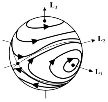
Figure 13.21.1:Rotation of an asymmetric rigid rotor. The dark lines correspond to contours of constant total rotational kinetic energy T, which has an ellipsoidal shape, projected onto the angular momentum L sphere in the body-fixed frame.

Assuming that the external torques are zero then the Euler equations of motion can be written as

\begin{align} I_1\dot{\omega}_1 = (I_2 − I_3) \omega_2\omega_3 \tag{13.156} \\ I_2\dot{\omega}_2 = (I_3 − I_1) \omega_3\omega_1 \notag \\ I_3\dot{\omega}_3 = (I_1 − I_2) \omega_1\omega_2 \notag \end{align}

Since $L_i = I_i\omega_i$ for $i = 1, 2, 3$ , then Equation 13.156 gives

\begin{align}I_2I_3\dot{L}_1 = (I_2 − I_3)L_2L_3 \tag{13.157} \\ I_1I_3\dot{L}_2 = (I_3 − I_1)L_3L_1 \notag \\ I_1I_2 \dot{L}_3 = (I_1 − I_2)L_1L_2 \notag \end{align}

Multiply the first equation by $I_1L_1$ , the second by $I_2L_2$ and the third by $I_3L_3$ and sum, which gives

I_1I_2I_3 \left( L_1\dot{L}_1 + L_2\dot{L}_2 + L_3\dot{L}_3 \right) = 0 \tag{13.158}

The bracket is equivalent to $\frac{d}{dt} (L^2_1 + L^2_2 + L^2_3)=0$ which implies that the total rotational angular momentum $L$ is a constant of motion as expected for this torque-free system, even though the individual components $L_1, L_2, L_3$ may vary. That is

L^2_1 + L^2_2 + L^2_3 = L^2 \tag{13.159}

Note that equation 13.159 is the equation of a sphere of radius $L$ .

Multiply the first equation of 13.157 by $L_1$ , the second by $L_2$ , and the third by $L_3$ , and sum gives

I_2I_3L_1\dot{L}_1 + I_1I_3L_2\dot{L}_2 + I_1I_2L_3\dot{L}_3 = 0 \tag{13.160}

Divide 13.160 by $I_1I_2I_3$ gives $\frac{d}{dt}( \frac{L^2_1}{2I_1} + \frac{L^2_2}{ 2I_2} + \frac{L^2_3}{2I_3} )=0$ . This implies that the total rotational kinetic energy $T$ , given by

\frac{L^2_1}{2I_1} + \frac{L^2_2}{2I_2} + \frac{L^2_3}{2I_3} = T \tag{13.161}

is a constant of motion as expected when there are no external torques and zero energy dissipation. Note that 13.161 is the equation of an ellipsoid.

Equations 13.159 and 13.161 both must be satisfied by the rotational motion for any value of the total angular momentum $\mathbf{L}$ and kinetic energy $T$ . Fig 13.21.1 shows a graphical representation of the intersection of the $L$ sphere and $T$ ellipsoid as seen in the body-fixed frame. The angular momentum vector $\mathbf{L}$ must follow the constant-energy contours given by where the $T$ -ellipsoids intersect the $L$ -sphere, shown for the case where $I_3 > I_2 > I_1$ . Note that the precession of the angular momentum vector $\mathbf{L}$ follows a trajectory that has closed paths that circle around the principal axis with the smallest $I$ , that is, $\hat{\mathbf{e}}_1$ , or the principal axis with the maximum $I$ , that is, $\hat{\mathbf{e}}_3$ . However, the angular momentum vector does not have a stable minimum for precession around the intermediate principal moment of inertia axis $\hat{\mathbf{e}}_2$ . In addition to the precession, the angular momentum vector $\mathbf{L}$ executes nutation, that is a nodding of the angle $\theta$ . For any fixed value of $L$ , the kinetic energy has upper and lower bounds given by

\frac{L^2}{2I_3} \leq T \leq \frac{L^2}{2I_1} \tag{13.162}

Thus, for a given value of $L$ , when $T = T_{\text{min}} = \frac{L^2}{2I_3}$ , the orientation of $\mathbf{L}$ in the body-fixed frame is either $(0, 0, +L)$ or $(0, 0, −L)$ , that is, aligned with the $\hat{\mathbf{e}}_3$ axis along which the principal moment of inertia is largest. For slightly higher kinetic energy the trajectory of $L$ follows closed paths precessing around $\hat{\mathbf{e}}_3$ . When the kinetic energy $T = \frac{L^2_2}{2I_2}$ the angular momentum vector $L$ follows either of the two thin-line trajectories each of which are a separatrix. These do not have closed orbits around $\hat{\mathbf{e}}_2$ and they separate the closed solutions around either $\hat{\mathbf{e}}_3$ or $\hat{\mathbf{e}}_1$ . For higher kinetic energy the precessing angular momentum vector follows closed trajectories around $\hat{\mathbf{e}}_1$ and becomes fully aligned with $\hat{\mathbf{e}}_1$ at the upper-bound kinetic energy.

Note that for the special case when $I_3 > I_2 = I_1$ , then the asymmetric rigid rotor equals the symmetric rigid rotor for which the solutions of Euler’s equations were solved exactly in chapter 13.19. For the symmetric rigid rotor the $T$ -ellipsoid becomes a spheroid aligned with the symmetry axis and thus the intersections with the $L$ -sphere lead to circular paths around the $\hat{\mathbf{e}}_3$ body-fixed principal axis, while the separatrix circles the equator corresponding to the $\hat{\mathbf{e}}_3$ axis separating clockwise and anticlockwise precession about $\mathbf{L}_3$ . This discussion shows that energy, plus angular momentum conservation, provide the general features of the solution for the torque-free symmetric top that are in agreement with those derived using Euler’s equations of motion.

13.22: Stability of torque-free rotation of an asymmetric body¶

It is of interest to extend the prior discussion to address the stability of an asymmetric rigid rotor undergoing force-free rotation close to a principal axes, that is, when subject to small perturbations. Consider the case of a general asymmetric rigid body with $I_3 > I_2 > I_1$ . Let the system start with rotation about the $\hat{\mathbf{e}}_1$ axis, that is, the principal axis associated with the moment of inertia $I_1$ . Then

\boldsymbol{\omega} = \omega_1 \widehat{\mathbf{e}}_1

Consider that a small perturbation is applied causing the angular velocity vector to be

\boldsymbol{\omega} =\omega_1 \widehat{\mathbf{e}}_1 + \lambda \widehat{\mathbf{e}}_2 + \mu \widehat{\mathbf{e}}_3

where $\lambda , \mu$ are very small. The Euler equations $(13.21.1)$ become

\begin{aligned} (I_2 − I_3) \lambda \mu − I_1\dot{\omega}_1 = 0 \\ (I_3 − I_1) \mu \omega_1 − I_2\dot{\lambda} = 0 \\ (I_1 − I_2) \omega_1 \lambda − I_3 \dot{\mu} = 0 \end{aligned}

Assuming that the product $\lambda \mu$ in the first equation is negligible, then $\dot{\omega}_1 = 0$ , that is, $\omega_1$ is constant.

The other two equations can be solved to give

\dot{\lambda} = \left(\frac{(I_3 − I_1)}{ I_2} \omega_1 \right) \mu

\dot{\mu} = \left(\frac{(I_1 − I_2)}{ I_3} \omega_1 \right) \lambda

Take the time derivative of the first equation

\ddot{\lambda} = \left(\frac{(I_3 − I_1)}{ I_2} \omega_1 \right) \dot{\mu}

and substitute for $\dot{\mu}$ gives

\ddot{\lambda} + \left(\frac{(I_1 − I_3) (I_1 − I_2)}{ I_2I_3} \omega^2_1 \right) \lambda = 0

The solution of this equation is

\lambda (t) = Ae^{i\Omega_{1\lambda}t} + Be^{-i\Omega_{1\lambda}t}

where

\Omega_{1\lambda} = \omega_1 \sqrt{\frac{(I_1 − I_3) (I_1 − I_2)}{I_2I_3}}

Note that since it was assumed that $I_3 > I_2 > I_1$ , then $\Omega_{1\lambda}$ is real. The solution for $\lambda (t)$ therefore represents a stable oscillatory motion with precession frequency $\Omega_{1\lambda}$ . The identical result is obtained for $\Omega_{1\mu} = \Omega_{1\lambda} = \Omega_1$ . Thus the motion corresponds to a stable minimum about the $\hat{\mathbf{e}}_1$ axis with oscillations about the $\lambda = \mu = 0$ minimum with period.

\Omega_1 = \omega_1 \sqrt{\frac{ (I_1 − I_3) (I_1 − I_2)}{ I_2I_3}} \tag{13.171}

Permuting the indices gives that for perturbations applied to rotation about either the 2 or 3 axes give precession frequencies

\Omega_2 = \omega_2 \sqrt{\frac{ (I_2 − I_1) (I_2 − I_3) }{I_1I_3}}

\Omega_3 = \omega_3 \sqrt{\frac{ (I_3 − I_2) (I_3 − I_1) }{I_1I_2 }} \tag{13.173}

Since $I_3 > I_2 > I_1$ then $\Omega_1$ and $\Omega_3$ are real while $\Omega_2$ is imaginary. Thus, whereas rotation about either the $I_3$ or the $I_1$ axes are stable, the imaginary solution about $\hat{\mathbf{e}}_2$ corresponds to a perturbation increasing with time. Thus, only rotation about the largest or smallest moments of inertia are stable. Moreover for the symmetric rigid rotor, with $I_1 = I_2 \neq I_3$ , stability exists only about the symmetry axis $\hat{\mathbf{e}}_3$ independent on whether the body is prolate or oblate. This result was implied from the discussion of energy and angular momentum conservation in chapter 13.20. Friction was not included in the above discussion. In the presence of dissipative forces, such as friction or drag, only rotation about the principal axis corresponding to the maximum moment of inertia is stable.

Stability of rigid-body rotation has broad applications to rotation of satellites, molecules and nuclei. The first U.S. satellite, Explorer 1, was launched in 1958 with the rotation axis aligned with the cylindrical axis which was the minimum principal moment of inertia. After a few hours the satellite started tumbling with increasing amplitude due to a flexible antenna dissipating and transferring energy to the perpendicular axis which had the largest moment of inertia. Torque-free motion of a deformed rigid body is a ubiquitous phenomena in many branches of science, engineering, and sports as illustrated by the following examples.

Example 13.22.1: Tennis racquet dynamics

Figure 13.22.1:Principal rotation axes for the center of mass of a tennis racket. The 1 and 2 -axes are in the plane of the racket head and the 3 axis is perpendicular to the plane of the racket head.

A tennis racquet is an asymmetric body that exhibits the above rotational behavior. Assume that the head of a tennis racquet is a uniform thin circular disk of radius $R$ and mass $M$ which is attached to a cylindrical handle of diameter $r = \frac{R}{10}$ , length $2R$ , and mass $M$ as shown in the figure. The principle moments of inertia about the three axes through the center-of-mass can be calculated by addition of the moments for the circular disk and the cylindrical handle and using both the parallel-axis and the perpendicular-axis theorems.

Axis	Head	Handle	Racquet
1	$\frac{1}{4} MR^2+MR^2= \frac{5}{4} MR^2$	$\frac{4}{3} MR^2$	$\frac{31}{12} MR^2$
2	$\frac{1}{4} MR^2+0= \frac{1}{4} MR^2$	$\frac{1}{200} MR^2$	$\frac{51}{200} MR^2$
3	$\frac{1}{2} MR^2+MR^2= \frac{3}{2} MR^2$	$\frac{4}{3} MR^2$	$\frac{17}{6} MR^2$

Note that $I_{11} : I_{22} : I_{33} = 2.5833 : 0.2550 : 2.8333$ . Inserting these principle moments of inertia into equations 13.171-13.173 gives the following precession frequencies

\Omega_1= i0 .8976\omega_1 \quad \Omega_2= 0 .9056\omega_2 \quad \Omega_3= 0 .9892\omega_3 \notag

The imaginary precession frequency $\Omega_1$ about the 1 axis implies unstable rotation leading to tumbling whereas the minimum moment $I_{22}$ and maximum moment $I_{33}$ imply stable rotation about the 2 and 3 axes. This rotational behavior is easily demonstrated by throwing a tennis racquet and is called the tennis racquet theorem. The center of percussion, example 2.12.8 is another important inertial property of a tennis racquet.

Example 13.22.2: Rotation of asymmetrically-deformed nuclei

Some nuclei and molecules have average shapes that have significant asymmetric deformation leading to interesting quantal analogs of the rotational properties of an asymmetrically-deformed rigid body. The major difference between a quantal and a classical rotor is that the energies, and angular momentum are quantized, rather than being continuously variable quantities. Otherwise, the quantal rotors exhibit general features similar to the classical analog. Studies [Cli86] of the rotational behavior of asymmetrically-deformed nuclei exploit three aspects of classical mechanics, namely classical Coulomb trajectories, rotational invariants, and the properties of ellipsoidal rigid-bodies.

Ellipsoidal deformation can be specified by the dimensions along each of the three principle axes. Bohr and Mottelson parameterized the ellipsoidal deformation in terms of three parameters, $R_0$ which is the radius of the equivalent sphere, $\beta$ which is a measure of the magnitude of the ellipsoidal deformation from the sphere, and $\gamma$ which specifies the deviation of the shape from axial symmetry. The ellipsoidal intrinsic shape can be expressed in terms of the deviation from the equivalent sphere by the equation

\delta R(\theta , \phi ) = R(\theta , \phi ) − R_0 = R_0 \sum^{\mu +2}_{ \mu =−2} \alpha^*_{2 \mu} Y_{2 \mu} (\theta , \phi ) \tag{a}

where $Y_{\lambda \mu} (\theta , \phi )$ is a Laplace spherical harmonic defined as

Y_{\lambda \mu} (\theta , \phi ) = \sqrt{\frac{ (2\lambda + 1) }{4\pi}\frac{ (\lambda − \mu )!}{ (\lambda + \mu )!}} P_{\lambda \mu} (\cos \theta )e^{-i\mu \phi} \notag

and $P_{\lambda \mu} (\cos \theta )$ is an associated Legendre function of $\cos \theta$ . Spherical harmonics are the angular portion of a set of solutions to Laplace’s equation. Represented in a system of spherical coordinates, Laplace’s spherical harmonics $Y_{\lambda \mu }(\theta , \phi )$ are a specific set of spherical harmonics that form an orthogonal system. Spherical harmonics are important in many theoretical and practical applications.

In the principal axis frame of the body, there are three non-zero quadrupole deformation parameters which can be written in terms of the deformation parameters $\beta , \gamma$ where $\alpha_{20} = \beta \cos \gamma$ , $\alpha_{21} = \alpha_{2−1} = 0$ , and $\alpha_{22} = \alpha_{2−2} = \frac{1}{\sqrt{2}}\beta \sin \gamma$ . Using these in equations alpha give the three semi-axis dimensions in the principal axis frame, (primed frame),

\delta R_k = \sqrt{\frac{5}{4\pi}} R_0\beta \cos (\gamma − \frac{2\pi k}{ 3 } ) \tag{b}

Note that for $\gamma = 0$ , then $\delta R_1 = \delta R_2 = −\frac{1}{2} \sqrt{\frac{5}{4\pi}} R_0\beta$ while $\delta R_3 = +\sqrt{\frac{5}{ 4\pi}} R_0\beta$ , that is the body has prolate deformation with the symmetry axis along the 3 axis. The same prolate shape is obtained for $\gamma = \frac{2\pi}{ 3}$ and $\gamma = \frac{4\pi}{ 3}$ with the prolate symmetry axes along the 1 and 2 axes respectively. For $\gamma = \frac{\pi}{ 3 }$ then $\delta R_1 = \delta R_3 = +\frac{1}{2} \sqrt{\frac{5}{4\pi}} R_0\beta$ while $\delta R2 = − \sqrt{\frac{5}{4\pi}} R_0\beta$ , that is the body has oblate deformation with the symmetry axis along the 2 axis. The same oblate shape is obtained for $\gamma = \pi$ and $\gamma = \frac{5\pi }{3}$ with the oblate symmetry axes along the 3 and 1 axes respectively. For other values of $\gamma$ the shape is ellipsoidal.

For the asymmetric deformed rigid body, the rotational Hamiltonian can be expressed in the form[Dav58]

H = \sum^3_{k=1 } \frac{|R|^2}{ 4B\beta^2 \sin^2(\gamma^{\prime} − \frac{2\pi k}{3}) }\notag

where the rotational angular momentum is $\mathbf{R}$ . The principal moments of inertia are related by the triaxiality parameter $\gamma^{\prime}$ which they assumed is identical to the shape parameter $\gamma$ . For axial symmetry the moment of inertia about the symmetry axis is taken to be zero for a quantal system since rotation of the potential well about the symmetry axis corresponds to no change in the potential well, or corresponding rotation of the bound nucleons. That is, the nucleus is not a rigid body, the nucleons only rotate to the extent that the ellipsoidal potential well is cranked around such that the nucleons must follow the rotation of the potential well. In addition, vibrational modes coexist about the average asymmetric deformation, plus octupole deformation often coexists with the above quadrupole deformed modes.

13.23: Symmetric rigid rotor subject to torque about a fixed point¶

The motion of a symmetric top rotating in a gravitational field, with one point at a fixed location, is encountered frequently in rotational motion. Examples are the gyroscope and a child’s spinning top. Rotation of a rigid rotor subject to torque about a fixed point, is a case where it is necessary to take the inertia tensor with respect to the fixed point in the body, and not at the center of mass.

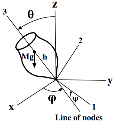
Figure 13.23.1:Symmetric top spinning about one fixed point.

Consider the geometry, shown in Figure 13.23.1, where the symmetric top of mass $M$ is spinning about a fixed tip that is displaced by a distance $h$ from the center of mass. The tip of the top is assumed to be at the origin of both the space-fixed frame $(x, y, z)$ and the body-fixed frame $(1, 2, 3)$ . Assume that the translational velocity is zero and let the principal moments about the fixed point of the symmetric top be $I_1 = I_2 \neq I_3$ .

The Lagrange equations of motion can be derived assuming that the kinetic energy equals the rotational kinetic energy, that is, it is assumed that the translational kinetic energy $T_{trans} = 0$ . Then the kinetic energy of an inertially-symmetric rigid rotor can be derived for the torque-free symmetric top as given in equation $(13.20.37)$ to be

\begin{align} T = \frac{1}{2} \sum_i I_i\omega^2_i = \frac{1}{2}I_1 (\omega^2_1 + \omega^2_2 )+ \frac{1}{ 2} I_3\omega^2_3 \\ = \frac{1}{2} I_1 \left( \dot{\phi}^2 \sin^2 \theta + \dot{\theta}^2 \right) + \frac{1}{2} I_3 \left( \dot{\phi} \cos \theta + \dot{\psi}\right)^2 \end{align}

Since the potential energy is $U = Mgh \cos \theta$ then the Lagrangian equals

L = \frac{1}{2} I_1 \left( \dot{\phi}^2 \sin^2 \theta + \dot{\theta}^2\right) + \frac{1}{2} I_3 \left( \dot{\phi} \cos \theta + \dot{\psi} \right)^2 − Mgh \cos \theta

The angular momentum about the space-fixed $z$ axis $p_{\phi}$ is conjugate to $\phi$ . From Lagrange’s equations

\dot{p}_{\phi} = \frac{\partial L}{\partial \phi} = 0

that is, $p_{\phi}$ is a constant of motion given by the generalized momentum

p_{\phi} = \frac{\partial L}{\partial \dot{\phi}} = ( I_1 \sin^2 \theta + I_3 \cos^2 \theta ) \dot{\phi} + I_3\dot{\psi} \cos \theta = S_z = \text{ constant}

where $S_z$ is the angular momentum projection along the space-fixed $z$ axis.

Similarly, the angular momentum about the body-fixed 3 axis is conjugate to $\psi$ . From Lagrange’s equations,

\dot{p}_{\psi} = \frac{\partial L}{ \partial \psi} = 0

that is, $p_{\psi}$ is a constant of motion given by the generalized momentum

p_{\psi} = \frac{\partial L}{ \partial \dot{\psi}} = I_3 \left( \dot{\dot{\phi}} \cos \theta + \dot{\psi} \right) = B_3 = \text{ constant}

where $B_3$ is the angular momentum projection along the body-fixed 3 axis. The above two relations can be solved to give the precessional angular velocity $\dot{\phi}$ about the space-fixed $z$ axis

\dot{\phi} = \frac{p_{\phi} − p_{\psi} \cos \theta}{ I_1 \sin^2 \theta }= \frac{S_z − B_3 \cos \theta}{ I_1 \sin^2 \theta}

and the spin angular velocity $\dot{\psi}$ about the body-fixed $x_3$ axis

\dot{\psi} = \frac{p_{\psi}}{I_3} − \frac{(p_{\phi} − p_{\psi} \cos \theta ) \cos \theta}{I_1 \sin^2 \theta} = \frac{B_3}{I_3} − \frac{(S_z − B_3 \cos \theta ) \cos \theta}{ I_1 \sin^2 \theta }

Since $p_{\phi}$ and $p_{\psi}$ are constants of motion, i.e. $S_3, B_3$ , then these rotational angular velocities depend on only $I_1$ , $I_3$ . and $\theta$ .

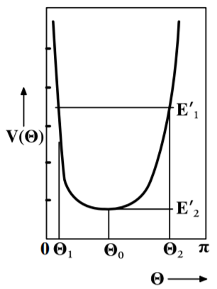
Figure 13.23.2:Effective potential diagram for a spinning symmetric top as a function of theta.

There is one further constant of motion available if no frictional forces act on the system, that is, energy conservation. This implies that the total energy

E = \frac{1}{ 2} I_1 \left( \dot{\phi}^2 \sin^2 \theta + \dot{\theta}^2 \right) + \frac{1}{2} I_3 \left( \dot{\phi} \cos \theta + \dot{\psi} \right)^2 + Mgh \cos \theta

will be a constant of motion. But the middle term on the right-hand side also is a constant of motion

\frac{1}{2} I_3 \left( \dot{\phi} \cos \theta + \dot{\psi} \right)^2 = \frac{p^2_{\psi}}{I_3} = \frac{B^2_3}{I_3} = \text{ constant}

Thus energy conservation can be rewritten by defining an energy $E^{\prime}$ where

E^{\prime} \equiv E − \frac{p^2_{\psi}}{ I_3} = \frac{1}{2} I_1 \left( \dot{\phi}^2 \sin^2 \theta + \dot{\theta}^2 \right) +Mgh \cos \theta = \text{ constant}

This can be written as

E^{\prime} = \frac{1}{2} I_1 \dot{\theta}^2 + \frac{(p_{\phi} − p_{\psi} \cos \theta )^2}{ 2I_1 \sin^2 \theta} + Mgh \cos \theta \tag{13.186}

which can be expressed as

E^{\prime} = \frac{1}{2} I_1 \dot{\theta}^2 + V (\theta )

where $V (\theta )$ is an effective potential

V (\theta ) \equiv \frac{(p_{\phi} − p_{\psi} \cos \theta )^2}{2I_1 \sin^2 \theta} + Mgh \cos \theta = \frac{(S_z − B_3 \cos \theta )^2}{ 2I_1 \sin^2 \theta} + Mgh \cos \theta \tag{13.188}

The effective potential $V (\theta )$ is shown in Figure 13.23.2. It is clear that the motion of a symmetric top with effective energy $E^{\prime}$ is confined to angles $\theta_1 < \theta < \theta_2$ . Note that the above result also is obtained if the Routhian is used, rather than the Lagrangian, as mentioned in chapter 8.7, and defined by equation $(8.6.8)$ . That is, the Routhian can be written as

R(\theta , \dot{\theta} , p_{\phi} p_{\psi} )_{cyclic} = \dot{\phi} p_{ \phi} + \dot{\psi} p_{ \psi} − L = H (\phi , p_{\phi} , \psi , p_{\psi }) − L(\theta , \dot{\theta} )_{noncyclic} \\ = −\frac{1}{2} I_1 \dot{\theta}^2 + \frac{(p_{\phi }− p_{\psi} \cos \theta )^2}{ 2I_1 \sin^2 \theta} + \frac{p^2_{\psi}}{ 2I_3 } + Mgh \cos \theta

The Routhian $R(\theta , \dot{\theta} , p_{\phi} p_{\psi} )_{cyclic}$ acts like a Hamiltonian for the $(\phi , p_{\phi} )$ and $(\psi , p_{\psi} )$ variables which are constants of motion, and thus are ignorable variables. The Routhian acts as the negative Lagrangian for the remaining variable $\theta$ , with rotational kinetic energy $\frac{1} {2} I_1 \dot{\theta}^2$ and effective potential energy $V_{eff}$

V_{eff} = \frac{(p_{\phi} − p_{\psi} \cos \theta )^2}{2I_1 \sin^2 \theta } + \frac{p^2_{\psi}}{ I_3} + Mgh \cos \theta = V (\theta ) + \frac{p^2_{\psi}}{ I_3 }\notag

The equation of motion describing the system in the rotating frame is given by one Lagrange equation

\frac{d}{dt}(\frac{ \partial R_{cyclic} }{\partial \dot{\theta}} ) − \frac{\partial R_{cyclic}}{ \partial \theta} = 0 \notag

The negative sign of the Routhian cancels out when used in the Lagrange equation. Thus, in the rotating frame of reference, the system is reduced to a single degree of freedom, the nutation angle $\theta$ , with effective energy $E^{\prime}$ given by equations 13.186 - 13.188.

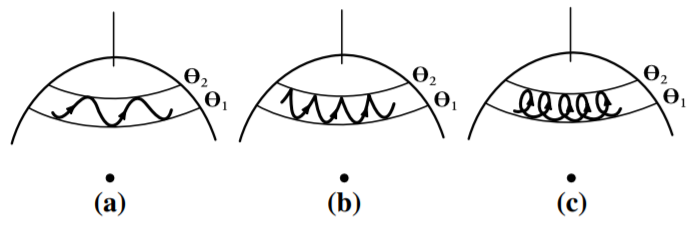
Nutational motion of the body-fixed symmetry axis projected onto the space-fixed unit sphere. The three case are (a) \dot{\phi} never vanishes, (b) \dot{\phi} = 0 at \theta = \theta_2 (c) \dot{\phi} changes sign between \theta_1 and \theta_2, — Figure 13.23.3:Nutational motion of the body-fixed symmetry axis projected onto the space-fixed unit sphere. The three case are (a) $\dot{\phi}$ never vanishes, (b) $\dot{\phi} = 0$ at $\theta = \theta_2$ (c) $\dot{\phi}$ changes sign between $\theta_1$ and $\theta_2$ ,

The motion of the symmetric top is simplest at the minimum value of the effective potential curve, where $E^{\prime} = V_{\text{min}}$ , at which the nutation $\theta$ is restricted to a single value $\theta = \theta_0$ . The motion is a steady precession at a fixed angle of inclination, that is, the “sleeping top”. Solving for $(\frac{dV}{d\theta} )_{\theta =\theta_0} = 0$ gives that

p_{\phi} − p_{\psi} \cos \theta = \frac{p_{\psi} \sin^2 \theta_0 }{2 \cos \theta_0} \left[ 1 \pm \sqrt{ 1 − \frac{4MghI_1 \cos \theta_0 }{p^2_{\psi}}} \right]

If $\theta_0 < \frac{\pi}{2}$ , then to ensure that the solution is real requires a minimum value of the angular momentum on the body-fixed axis of $p^2_{\psi} \geq 4MghI_1 \cos \theta_0$ . If $\theta_0 > \frac{\pi}{2}$ then there is no minimum angular momentum projection on the body-fixed axis. There are two possible solutions to the quadratic relation corresponding to either a slow or fast precessional frequency. Usually the slow precession is observed.

For the general case, where $E^{\prime}_1 > V_{\text{min}}$ , the nutation angle $\theta$ between the space-fixed and body-fixed 3 axes varies in the range $\theta_1 < \theta < \theta_2$ . This axis exhibits a nodding variation which is called nutation. Figure 13.23.3 shows the projection of the body-fixed symmetry axis on the unit sphere in the space-fixed frame. Note that the observed nutation behavior depends on the relative sizes of $p_{\phi}$ and $p_{\psi} \cos \theta$ . For certain values, the precession $\dot{\phi}$ changes sign between the two limiting values of $\theta$ producing a looping motion as shown in Figure 13.23.3c. Another condition is where the precession is zero for $\theta_2$ producing a cusp at $\theta_2$ as illustrated in Figure 13.23.3b. This behavior can be demonstrated using the gyroscope or the symmetric top.

Example 13.23.1: The Spinning “Jack”

Figure 13.23.4:Jack comprises six bodies of mass $m$ at each end of orthogonal arms of length $l$

The game “Jacks” is played using metal Jacks, each of which comprises six equal masses $m$ at the opposite ends of orthogonal axes of length $l$ . Consider one jack spinning around the body-fixed 3−axis with the lower mass at a fixed point on the ground, and with a steady precession around the space-fixed vertical axis $z$ with angle $\theta$ as shown. Assume that the body-fixed axes align with the arms of the jack.

The principal moments of inertia about one mass is given by the parallel axis theorem to be $I_2 = I_1 = 4ml^2+6ml^2 = 10ml^2$ and $I_3 = 4ml^2$ .

In the rotating body-fixed frame the torque due to gravity has components

\mathbf{N} = \begin{pmatrix} 6mgl \sin \theta \sin\psi \\ 6mgl \sin \theta \cos \psi \\ 0 \end{pmatrix}\notag

and the components of the angular velocity are

\boldsymbol{\omega} = \begin{pmatrix} \dot{\phi} \sin \theta \sin\psi + \dot{\theta} \cos \psi \\ \dot{\phi} \sin \theta \cos \psi − \dot{\theta} \sin \\ \dot{\phi} \cos \theta + \dot{\psi} \end{pmatrix} \notag

Using Euler’s equations $(13.17.6)$ for the above components of $N$ and $\omega$ in the body-fixed frame, gives

10\dot{\omega}_1 − 6\omega_2\omega_3 = \frac{6g}{l} \sin \theta \sin \psi \tag{a}

10\dot{\omega}_2 − 6\omega_1\omega_3 = \frac{6g}{l} \sin \theta \cos \psi \tag{b}

4\dot{\omega}_3 = 0 \tag{c}

Equation c relates the spin about the 3 axis, the precession, and the angle to the vertical $\theta$ , that is

\omega_3 = \dot{\phi} \cos \theta + \dot{\psi} = \Omega \cos \theta + s = \text{ constant}

where $\dot{\psi} \equiv s$ is the spin and $\dot{\phi} \equiv \Omega$ is the precession angular velocity.

If the spin axis is nearly vertical, $\theta \approx 0$ and thus $\sin \theta \approx \theta$ and $\cos \theta \approx 1$ . Multiply Equation a $\times \sin\psi +\text{(b)}\times \cos \psi$ and using the equations of the components of $\omega$ gives

5\ddot{\theta} + \left( 2\Omega s − 3\Omega^2 − \frac{3g}{l} \right) \theta = 0 \notag

The bracket must be positive to have stable sinusoidal oscillations. That is, the spin angular velocity $s$ required for the jack to spin about a stable vertical axis is given by.

s > \frac{3\Omega}{2} + \frac{3g}{2l \Omega}\notag

This example illustrates the conditions required for stable rotation of any axially-symmetric top.

Example 13.23.2: The Tippe Top

Figure 13.23.5:The geometry of the Tippe Top of radius $R$ spinning on a horizontal surface with slipping friction acting between the top and the horizontal plane. The center of mass is a distance $a$ from the center of the spherical section along the axis of symmetry of the top.

The Tippe Top comprises a section of a sphere, to which a short cylindrical rod is mounted on the planar section, as illustrated. When the Tippe Top is spun on a horizontal surface this top exhibits the perverse behavior of transitioning from rotation with the spherical head resting on the horizontal surface, to flipping over such that it rotates resting on its elongated cylindrical rod. The orientation of angular momentum remains roughly vertical as expected from conservation of angular momentum. This implies that the rotation with respect to the body-fixed axes must invert as the top inverts. The center of mass is raised when the top inverts; the additional potential energy is provided by a reduction in the rotational kinetic energy.

The Tippe Top behavior was first discovered in the 1890’s but adequate solutions of the equations of motion have only been developed since the 1950’s. Since the top precesses around the vertical axis, the point of contact is not on the symmetry axis of the top. Sliding friction between the surface of the spinning top and the horizontal surface provides a torque that causes the precession of the top to increase and eventually flip up onto the cylindrical peg. The Tippe Top is typical of many phenomena in physics where the underlying physics principle can be recognized but a detailed and rigorous solution can be complicated.

The system has five degrees of freedom, $x,y$ which specify the location on the horizontal plane, plus the three Euler angles $(\varphi, \theta , \phi )$ . The paper by Cohen[Coh77] explains the motion in terms of Euler angles using the laboratory to body-fixed transformation relation. It shows that friction plays a pivotal role in the motion contrary to some earlier claims. Ciocci and Langerock[Cio07] used the Routhian $R_{cyclic}$ to reduce the number of degrees of freedom from 5 to 2, namely $\theta$ which is the tilt angle, and $\varphi^{\prime}$ which is the orientation of the tilt. This Routhian $R_{cyclic}$ is a Lagrangian in two dimension that was used to derive the equations of motion via the Lagrange Euler equation

\begin{aligned} \frac{d}{dt}( \frac{ \partial R_{cyclic} }{\partial \dot{\theta} }) − \frac{\partial R_{cyclic} }{\partial \theta} = Q_{\theta} \\ \frac{d}{dt}( \frac{\partial R_{cyclic}}{ \partial \dot{\varphi}^{\prime}}) − \frac{\partial R_{cyclic}}{ \partial \varphi^{\prime}} = Q_{\varphi^{\prime}}\end{aligned}

where the $Q_{\theta} \ Q_{\varphi^{\prime}}$ are generalized torques about the 2 angles that take into account the sliding frictional forces. This sophisticated Routhian reduction approach provides an exhaustive and refined solution for the Tippe Top and confirms that sliding friction plays a key role in the unusual behavior of the Tippe Top.

13.24: The Rolling Wheel¶

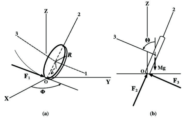
As discussed in chapter 5.7, the rolling wheel is a non-holonomic system that is simple in principle, but in practice the solution can be complicated, as illustrated by the Tippe Top. Chapter 13.23 discussed the motion of a symmetric top rotating about a fixed point on the symmetry axis when subject to a torque. The rolling wheel involves rotation of a symmetric rigid body that is subject to torques. However, the point of contact of the wheel with a static plane is on the periphery of the wheel, and friction at the point of contact is assumed to ensure zero slip. Note that friction is necessary to ensure that the rotating object rolls without slipping, but the frictional force does no work for pure rolling of an undeformable rigid wheel.

The coordinate system employed is shown in Figure 13.24.1. For simplicity it is better to use a moving coordinate frame $(\mathbf{1},\mathbf{2},\mathbf{3})$ that is fixed to the orientation of the wheel with the origin at the center of mass of the wheel, but this moving reference frame does not include the angular velocity $\dot{\psi}$ of the disk about the $\mathbf{3}$ axis. That is, the moving $(\mathbf{1},\mathbf{2},\mathbf{3})$ frame has angular velocities

\begin{align} \omega_1 = \dot{\theta} \tag{13.191} \\ \omega_2 = \dot{\phi} \sin \theta \notag\\ \omega_3 = \dot{\phi} \cos \theta \notag\end{align}

The frame fixed in the rotating wheel must include the additional angular velocity of the disk $\dot{\psi}$ about the $\mathbf{\hat{e}}_3$ axis, that is

\begin{align}\Omega_1 = \omega_1 = \dot{\theta} \tag{13.192} \\ \Omega_2 = \omega_2 = \dot{\phi} \sin \theta \notag\\ \Omega_3 = \omega_3 + \dot{\psi} = \dot{\phi} \cos \theta + \dot{\psi} \notag\end{align}

where $\Omega$ designates the angular velocity of the rotating disk, while $\boldsymbol{\omega}$ designates the rotation of the moving frame $(\mathbf{1},\mathbf{2},\mathbf{3})$ .

The principle moments of inertia of a thin circular disk are related by the perpendicular axis theorem (chapter 13.9)

I_1 + I_2 = I_3 \notag

Since $I_1 = I_2$ for a uniform disk, therefore $I_3 = 2I_1$ .

Equation $(12.3.10)$ can be used to relate the vector forces $\mathbf{F}$ in the space-fixed frame to the rate of change of momenta in the moving frame $(\mathbf{1},\mathbf{2},\mathbf{3})$ .

\mathbf{F} = \mathbf{\dot{p}}_{space} = \mathbf{\dot{p}}_{moving} + \boldsymbol{\omega} \times \mathbf{p} \tag{13.193}

This leads to the following relations for the three components in the moving frame

\begin{align}F_1 = \dot{p}_1 + \omega_2 p_3 − \omega_3 p_2 \tag{13.194} \\ F_2 − Mg \sin \theta = \dot{p}_2 + \omega_3 p_1 − \omega_1 p_3 \notag\\ F_3 − Mg \cos \theta = \dot{p}_3 + \omega_1 p_2 − \omega_2 p_1 \notag\end{align}

where $F_1, F_2, F_3$ are the reactive forces acting shown in Figure 13.24.1.

Uniform disk rolling on a horizontal plane as viewed in the (a) fixed frame, and (b) rolling disk frame. The space-fixed axis system is (\mathbf{x}, \mathbf{y}, \mathbf{z}), while the moving reference frame (\mathbf{1},\mathbf{2},\mathbf{3}) is centered at the center of mass of the disk with the … — Figure 13.24.1:Uniform disk rolling on a horizontal plane as viewed in the (a) fixed frame, and (b) rolling disk frame. The space-fixed axis system is $(\mathbf{x}, \mathbf{y}, \mathbf{z})$ , while the moving reference frame $(\mathbf{1},\mathbf{2},\mathbf{3})$ is centered at the center of mass of the disk with the $\mathbf{1}, \mathbf{2}$ axes in the plane of the disk. The disk is rotating with a uniform angular velocity $\dot{\psi}$ about the $\mathbf{3}$ axis and rolling in the direction that is at an angle $\phi$ relative to the $x$ axis.

Similarly, the torques $\mathbf{N}$ in the space-fixed frame can be related to the rate of change of angular momentum by

\mathbf{N} = \mathbf{\dot{L}}_{space} = \mathbf{\dot{L}}_{moving} + \boldsymbol{\omega} \times \mathbf{L} \tag{13.195}

where $L_i = \mathbf{I}_i\Omega _i$ . This leads to the following relations for the three torque equations in the moving frame

\begin{align}N_1 = −F_3 R = I_1 \dot{\Omega}_1 + I_3\Omega_3\omega_2 − I_2\Omega 2\omega_3 \tag{13.196} \\ N_2 = 0 = I_1 \dot{\Omega}_2 + I_1 \Omega_1 \omega_3 − I_3\Omega_3\omega_1 \notag\\ N_3 = F_1 R = I_3 \dot{\Omega}_3 + I_2 \Omega_2 \omega_1 − I_1\Omega_1 \omega_2 \notag\end{align}

The rolling constraints are

p_1 + MR \Omega_3 = 0 \tag{13.197} \\ p_2 = 0 \\ p_3 − MR \Omega_1 = 0

where $p_i = Mv_i$ . Combining equations 13.194, 13.196, 13.197 gives

\begin{align}(I_1 + MR^2) \dot{\Omega}_1 + ( I_3 + MR^2) \omega_2\Omega_3 − I_2\omega_3\Omega_2 = −MgR \cos \theta \tag{13.198} \\ I_1\dot{\Omega}_2 + I_1\omega_3\Omega_1 − I_3\omega_1\Omega_3 = 0 \notag\\ ( I_3 + MR^2) \dot{\Omega}_3 + I_2\omega_1\Omega_2 − ( I_1 + MR^2) \omega_2\Omega_1 = 0 \notag\end{align}

These are the torque equations about the point of contact $O$ .

Introduction of equations 13.191 and 13.192 into Equation 13.198 expresses the equations of motion in terms of the Euler angles to be

\begin{align}( I_1 + MR^2) \ddot{\theta} + ( I_3 + MR^2) \dot{\phi} \sin \theta \left( \dot{\phi} \cos \theta + \dot{\psi}\right)− I_1\dot{\phi}^2 \sin \theta \cos \theta = −MgR \cos \theta \tag{13.199} \\ \notag I_1 \ddot{\phi} \sin \theta + 2I_1\dot{\phi} \dot{\theta} \cos \theta − I_3 \dot{\theta} \left( \dot{\phi} \cos \theta + \dot{\psi}\right)= 0 \\ \notag ( I_3 + MR^2) \left( \ddot{\phi} \cos \theta − \dot{\phi} \dot{\theta} \sin \theta + \ddot{\psi} \right)− MR^2 \dot{\theta}\dot{\phi} \sin \theta = 0 \end{align}

Equations 13.199 are non-linear, and a closed-form solution is possible only for limited cases such as when $\theta = 90^{\circ}$ .

Note that the above equations of motion also can be derived using Lagrangian mechanics knowing that

L = \frac{1}{2} M ( v^2_1 + v^2_2 + v^2_3 ) + \frac{1}{2} I_1 ( \Omega^2_1 + \Omega^2_2 ) + \frac{1}{2} I_3\Omega^2_3 − MgR \cos \theta \notag

The differential equations of constraint can be derived from equations 13.197 to be

dx − R \cos \phi d\psi = 0 \notag

dy − R \sin \phi d\psi = 0

Use of generalized forces plus the Lagrange-Euler equations $(6.3.28)$ can be used to derive the equations of motion and solve for the components of the constraint force $F_1$ , $F_2$ , and $F_3$ .

Example 13.24.1: Tipping stability of a rolling wheel

A circular wheel rolling in a vertical plane at high angular velocity initially rolls in a straight line and remains vertical. However, below a certain angular velocity, gyroscopic forces become weaker and the wheel will tip sideways and veer rapidly from the initial direction. It is interesting to estimate the minimum angular velocity of the disk such that it does not start to tip over sideways.

Note that equations 13.199 are satisfied for $\theta = \frac{\pi}{2}$ , $\phi = 0$ and $\dot{\psi} = \Omega_3 =$ constant. Assume a small disturbance causes the tilt angle to be $\theta = \frac{\pi}{2} + \alpha$ where $\alpha$ is small and that $\phi$ is non-zero but small, that is $\dot{\theta} = \dot{\alpha}$ and $\dot{\phi}$ are small. Keeping only terms to first order in the third of equations 13.199, and integrating gives

\dot{\phi} \cos \theta + \dot{\psi} = \Omega_3 \tag{a}

The first two of equations 13.198 become

( I_1 + MR^2) \ddot{\alpha} + ( I_3 + MR^2) \dot{\phi} \Omega_3 − MgR\alpha = 0 \tag{b}

I_1 \ddot{\phi} − I_3\Omega_3 \dot{\alpha} = 0 \tag{c}

Integrating Equation c gives

\dot{\phi} = \frac{I_3\Omega_3}{ I_1 } \alpha \tag{d}

Inserting d into b gives

( I_1 + MR^2) \ddot{\alpha} + \left[ ( I_3 + MR^2) \frac{I_3\Omega^2_3}{ I_1 } − MgR \right] \alpha = 0 \tag{e}

Equation e has a stable oscillatory solution when the square bracket in positive, that is,

\Omega^2_3 > \frac{I_1MgR}{ I_3 (I_3 + MR^2)} \tag{f}

which gives the minimum angular velocity required for stable rolling motion. For angular velocity less than the minimum, the square bracket in Equation e is negative leading to an exponentially decaying and divergent solution. For a uniform disk the perpendicular axis theorem gives $I_3 = 2I_1 = \frac{1}{2} MR^2$ for which Equation f gives

\Omega^2_3 \frac{g}{3R} \tag{g}

Therefore the critical linear velocity of the wheel is

v = R\Omega_3 > \sqrt{\frac{gR}{3}} \tag{h}

The bicycle wheel provides a common example of the tipping of a rolling wheel. For the typical 0.35 $m$ radius of a bicycle wheel, this gives a critical velocity of $v > 1.07$ $m/s$ $= 2.4$ $mph$ .^[4]

13.25: Dynamic balancing of wheels¶

For rotating machinery It is crucial that rotors be both statically and dynamically balanced. Static balance means that the center of mass is on the axis of rotation. Dynamic balance means that the axis of rotation is a principal axis.

For example, consider the symmetric rotor that has its symmetry axis at an angle $\phi$ to the axis of rotation. In this case the system is statically balanced since the center of gravity is on the axis of rotation. However, the rotation axis is at an angle $\phi$ to the symmetry axis. This implies that the axle has to provide a torque to maintain rotation that is not along a principal axis. If you distort the front wheel of your car by hitting it sideways against the sidewalk curb, or if the wheel is not dynamically balanced, then you will find that the steering wheel can vibrate wildly at certain speeds due to the torques caused by dynamic imbalance shaking the steering mechanism. This can be especially bad when the rotation frequency is close to a resonant frequency of the suspension system. Insist that your automobile wheels are dynamically balanced when you change tires, static balancing will not eliminate the dynamic imbalance forces. Another example is that the ailerons, rudder, and elevator on aircraft usually are dynamically balanced to stop the build up of oscillations that can couple to flexing and flutter of the airframe which can lead to airframe failure.

Example 13.25.1: Forces on the bearings of a rotating circular disk

$Rotation of circular disk about an axis that is at an angle \alpha to the symmetry axis of the circular disk.$

Figure 13.25.1:Rotation of circular disk about an axis that is at an angle $\alpha$ to the symmetry axis of the circular disk.

A homogeneous circular disk of mass $M$ , and radius $R$ , rotates with constant angular velocity $\omega$ about a body-fixed axis passing through the center of the circular disk as shown in the adjacent figure. The rotation axis is inclined at an angle $\alpha$ to the symmetry axis of the circular disk by bearings on both sides of the disk spaced a distance $d$ apart. Determine the forces on the bearings.

Choose the body-fixed axes such that $\hat{e}_3$ is along the symmetry axis of the circular disk, and $\hat{e}_1$ points in the plane of the disk symmetry axis and the rotation axis. These axes are the principal axes for which the inertia tensor can be calculated to be

\mathbf{I} = \frac{MR^2}{4} \begin{pmatrix} 1 & 0 & 0 \\ 0 & 1 & 0 \\ 0 & 0 & 2\end{pmatrix} \notag

Note that for this thin plane laminae disk $I_{11} + I_{22} = I_{33}$ .

The components of the angular velocity vector $\omega$ along the three body-fixed axes are given by

\boldsymbol{\omega} = (\omega \sin \alpha , 0,\omega \ cos \alpha ) \notag

Since it is assumed that $\dot{\omega} = 0$ then substituting into Euler’s equations $(13.17.6)$ gives the torques acting to be

N_1 = N_3 = 0 \\ N_2 = −\omega^2 \sin \alpha \cos \alpha \frac{1}{4} MR^2\notag

That is, the torque is in the $\hat{e}_2$ direction. Thus the forces $F$ on the bearings can be calculated since $\mathbf{N} = \mathbf{r} \times \mathbf{F}$ , thus

|F| = \frac{|N_2|}{ 2d} = MR^2\omega^2 \frac{\sin 2\alpha}{16d}\notag

Estimate the size of these forces for the front wheel of your car travelling at 70 $m.p.h.$ if the rotation axis is displaced by $2^{\circ}$ from the symmetry axis of the wheel.

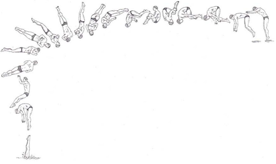
Forward two-and-a-half somersaults with two twists demonstrates unequivocally that a diver can initiate continuous twisting in midair. In the illustrated maneuver the diver does more than one full somersault before he starts to twist. To maintain the twisting the diver does not have to move his l… — Figure 13.25.2:Forward two-and-a-half somersaults with two twists demonstrates unequivocally that a diver can initiate continuous twisting in midair. In the illustrated maneuver the diver does more than one full somersault before he starts to twist. To maintain the twisting the diver does not have to move his legs.[Fro80]

13.26: Rotation of Deformable Bodies¶

The discussion in this chapter has assumed that the rotating body is a rigid body. However, there is a broad and important class of problems in classical mechanics where the rotating body is deformable that leads to intriguing new phenomena. The classic example is the cat, which, if dropped upside down with zero angular momentum, is able to distort its body plus tail in order to rotate such that it lands on its feet in spite of the fact that there are no external torques acting and thus the angular momentum is conserved. Another example is the high diver doing a forward two—and-a-half somersault with two twists.[Fro80] Once the diver leaves the board then the total angular momentum must be conserved since there are no external torques acting on the system. The diver begins a somersault by rotating about a horizontal axis which is a principal axis that is perpendicular to the axis of his body passing through his hips. Initially the angular momentum, and angular velocity, are parallel and point perpendicular to the symmetry axis. Initially the diver goes into a tuck which greatly reduces his moment of inertia along the axis of his somersault which concomitantly increases his angular velocity about this axis and he performs one full somersault prior to initiating twisting. Then the diver twists its body and moves its arms to destroy the axial symmetry of his body which changes the direction of the principal axes of the inertia tensor. This causes the angular velocity to change in both direction and magnitude such that the angular momentum remains conserved. The angular velocity now is no longer parallel to the angular momentum resulting in a component along the length of the body causing it to twist while somersaulting. This twisting motion will continue until the symmetry of the diver’s body is restored which is done just before entering the water. By skilled timing, and body movement, the diver restores the symmetry of his body to the optimum orientation for entering the water. Such phenomena involving deformable bodies are important to motion of ballet dancers, jugglers, astronauts in space, and satellite motion. The above rotational phenomena would be impossible if the cat or diver were rigid bodies having a fixed inertia tensor. Calculation of the dynamics of the motion of deformable bodies is complicated and beyond the scope of this book, but the concept of a time dependent transformation of the inertia tensor underlies the subsequent motion. The theory is complicated since it is difficult even to quantify what corresponds to rotation as the body morphs from one shape to another. Further information on this topic can be found in the literature. [Fro80]

13.E: Rigid-body Rotation (Exercises)¶

A hollow spherical shell has a mass $m$ and radius $R$ .
Calculate the inertia tensor for a set of coordinates whose origin is at the center of mass of the shell.
Now suppose that the shell is rolling without slipping toward a step of height $h$ , where $h < R$ . The shell has a linear velocity $v$ . What is the angular momentum of the shell relative to the tip of the step?
The shell now strikes the tip of the step inelastically (so that the point of contact sticks to the step, but the shell can still rotate about the tip of the step). What is the angular momentum of the shell immediately after contact?
Finally, find the minimum velocity which enables the shell to surmount the step. Express your result in terms of $m$ , $g$ , $R$ , and $h$ .
The vectors $\hat{x}$ , $\hat{y}$ , and $\hat{z}$ constitute a set of orthogonal right-handed axes. The vectors $\hat{x} + \hat{y} − 2\hat{z}$ , $−\hat{x} + \hat{y}$ , and $\hat{x} + \hat{y} + \hat{z}$ are also perpendicular to one another.
Write out the set of direction cosines relating the new axes to the old.
How are the Eulerian angles defined? Describe this transformation by a set of Eulerian angles.
A torsional pendulum consists of a vertical wire attached to a mass which can rotate about the vertical axis. Consider three torsional pendula which consist of identical wires from which identical homogeneous solid cubes are hung. One cube is hung from a corner, one from midway along an edge, and one from the middle of a face as shown. What are the ratios of the periods of the three pendula?

A dumbbell comprises two equal point masses $M$ connected by a massless rigid rod of length $2A$ which is constrained to rotate about an axle fixed to the center of the rod at an angle $\theta$ as shown in the figure. The center of the rod is at the origin of the coordinates, the axle along the $z$ -axis, and the dumbbell lies in the $x-y$ plane at $t = 0$ . The angular velocity $\omega$ is a constant in time and is directed along the $z$ axis.
Calculate all elements of the inertia tensor. Be sure to specify the coordinate system used.
Using the calculated inertia tensor find the angular momentum of the dumbbell in the laboratory frame as a function of time.
Using the equation $L = r \times p$ , calculate the angular momentum and show that it is equal to the answer of part (b).
Calculate the torque on the axle as a function of time.
Calculate the kinetic energy of the dumbbell.

A heavy symmetric top has a mass $m$ with the center of mass a distance $h$ from the fixed point about which it spins and $I_1 = I_2 \neq I_3$ . The top is precessing at a steady angular velocity $\Omega$ about the vertical space-fixed $z$ axis. What is the minimum spin $\omega^{\prime}$ about the body-fixed symmetry axis, that is, the 3 axis assuming that the 3 axis is inclined at an angle $\theta = \theta$ with respect to the vertical $z$ axis. Solve the problem at the instant when the $z, x, 3, 1$ axes all are in the same plane as shown in the figure.

Consider an object with the center of mass is at the origin and inertia tensor,
$I = I \begin{pmatrix} 1/2 & -1/2 & 0 \\ -1/2 & 1/2 & 0 \\ 0 & 0 & 1 \end{pmatrix}\nonumber$
Determine the principal moments of inertia and the principal axes. Guess the object.
Determine the rotation matrix $R$ and compute $R^{\dagger}IR$ . Do the diagonal elements match with your results from (a)? Note: columns of $R$ are eigenvectors of $I$ .
Assume $\omega = \frac{\omega}{\sqrt{2}} (\hat{x} + \hat{z})$ . Determine $L$ in the rotating coordinate system. Are $L$ and $\omega$ in the same direction? What does this mean?
Repeat (c) for $\omega = \frac{\omega}{\sqrt{ 2}} (\hat{x} − \hat{y})$ . What is different and why?
For which case will there be a non-zero torque required?
Determine the rotational kinetic energy for the case $\omega = \frac{\omega}{\sqrt{ 2}} (\hat{x} − \hat{y})$ ?
Consider a wheel (solid disk) of mass $m$ and radius $r$ . The wheel is subject to angular velocities $\omega_A = \omega_A \hat{n}$ where $\hat{n}$ is normal to the surface and $\omega_B = \omega_B \hat{z}$ .

Choose a set of principal axes by observation.
Determine the angular velocities and angular momentum along the principal axes. Note: $I_1 = \frac{1}{2} mr^2$ and $I_2 = I_3 = \frac{1}{4}mr^2$ .
Determine the torque.
Determine the rotation matrix that rotates the fixed coordinate system to the body coordinate system.
Determine the principal moments of inertia of an ellipsoid given by the equation,
$\frac{x^2}{a^2} + \frac{y^2}{b^2} + \frac{z^2}{c^2} = 1.\nonumber$
Determine the principal moments of inertia of a sphere of radius $R$ with a cavity of radius $r$ located $\epsilon$ from the center of the sphere.
Three equal masses $m$ form the vertices of an equilateral triangle of side length $L$ . Assume that the masses are located at $\left( 0, 0, \frac{L}{\sqrt{3}}\right)$ , $\left( 0, \frac{L}{2}, − \frac{L}{ 2 \sqrt{3}}\right)$ , and $\left( 0, -\frac{L}{2}, − \frac{L}{ 2 \sqrt{3}}\right)$ , such that the center-of-mass is located at the origin.
Determine the principal moments of inertia and principal axes.

Now consider the same system rotated $45^{\circ}$ about the $\hat{z}$ -axis. Assume that the masses are located at $\left( 0, 0, \frac{L}{\sqrt{3}}\right)$ , $\left( -\frac{L}{2\sqrt{2}}, \frac{L}{2\sqrt{2}}, − \frac{L}{ 2 \sqrt{3}}\right)$ , and $\left( \frac{L}{2\sqrt{2}}, -\frac{L}{2\sqrt{2}}, − \frac{L}{ 2 \sqrt{3}}\right)$ , respectively.

Determine the principal moments of inertia and principal axes.
Could you have answered (b) without explicitly determining the inertia tensor? How?
Calculate the moments of inertia $I_1, I_2, I_3$ for a homogeneous cone of mass $M$ whose height is $h$ and whose base has a radius $R$ . Choose the $x_3$ -axis along the symmetry axis of the cone.
Choose the origin at the apex of the cone, and calculate the elements of the inertia tensor.
Make a transformation such that the center of mass of the cone is the origin and find the principal moments of inertia.
Four masses, all of mass $m$ , lie in the $x − y$ plane at positions $(x, y)=(a, 0),(−a, 0),(0, +2a),(0, −2a)$ . These are joined by massless rods to form a rigid body
Find the inertial tensor, using the $x, y, z$ axes as a reference system. Exhibit the tensor as a matrix.
Consider a direction given by the unit vector $\hat{n}$ that lies equally between the positive $x, y, z$ axes; that is it makes equal angles with these three directions. Find the moment of inertia for rotation about this $\hat{n}$ axis.
Given that at a certain time $t$ the angular velocity vector lies along the above direction $\hat{n}$ , find, for that instant, the angle between the angular momentum vector and $\hat{n}$ .
A homogeneous cube, each edge of which has a length $l$ , initially is in a position of unstable equilibrium with one edge of the cube in contact with a horizontal plane. The cube then is given a small displacement causing it to tip over and fall. Show that the angular velocity of the cube when one face strikes the plane is given by
$\omega^2 = A\frac{g}{l} \left( \sqrt{2} - 1 \right) \nonumber$
where $A = \frac{3}{2}$ if the edge cannot slide on the plane, and where $A = \frac{12}{5}$ if sliding can occur without friction.
A symmetric body moves without the influence of forces or torques. Let $x_3$ be the symmetry axis of the body and $L$ be along $x^{\prime}_3$ . The angle between $\omega$ and $x_3$ is $\alpha$ . Let $\omega$ and $L$ initially be in the $x_2 − x_3$ plane. What is the angular velocity of the symmetry axis about $L$ in terms of $I_1$ , $I_3$ , $\omega$ , and $\alpha$ ?
Consider a thin rectangular plate with dimensions $a$ by $b$ and mass $M$ . Determine the torque necessary to rotate the thin plate with angular velocity $\omega$ about a diagonal. Explain the physical behavior for the case when $a = b$ .

13.S: Rigid-body Rotation (Summary)¶

This chapter has introduced the important, topic of rigid-body rotation which has many applications in physics, engineering, sports, etc.

Inertia tensor¶

The concept of the inertia tensor was introduced where the 9 components of the inertia tensor are given by

I_{ij} = \int\rho (\mathbf{r}^{\prime} ) \left( \delta_{ij} \left( \sum^3_k x^2_{k} \right) − x_{i} x_{ j} \right) dV

Steiner’s parallel-axis theorem

J_{11} \equiv I_{11} + M((a^2_1 + a^2_2 + a^3_3) \delta_{11} - a^2_1) = I_{11} + M(a^2_2 + a^2_3)

relates the inertia tensor about the center-of-mass to that about parallel axis system not through the center of mass.

Diagonalization of the inertia tensor about any point was used to find the corresponding Principal axes of the rigid body.

Angular momentum¶

The angular momentum $\mathbf{L}$ for rigid-body rotation is expressed in terms of the inertia tensor and angular frequency $\omega$ by

\mathbf{L} = \begin{pmatrix} I_{11} & I_{12} & I_{13} \\ I_{21} & I_{22} & I_{23} \\ I_{31} & I_{32} & I_{33} \end{pmatrix} \cdot \begin{pmatrix} \omega_1 \\ \omega_2 \\ \omega_3 \end{pmatrix} = \{\mathbf{I}\} \cdot \boldsymbol{\omega} \tag{13.55}

Rotational kinetic energy¶

The rotational kinetic energy is

T_{rot} = \frac{1}{2} \left( \omega_1 \ \omega_2 \ \omega_3 \right) \cdot \begin{pmatrix} I_{11} & I_{12} & I_{13} \\ I_{21} & I_{22} & I_{23} \\ I_{31} & I_{32} & I_{33} \end{pmatrix} \cdot \begin{pmatrix} \omega_1 \\ \omega_2 \\ \omega_3 \end{pmatrix}

T_{rot} \equiv \mathbf{T} = \frac{1}{2} \boldsymbol{\omega} \cdot \{\mathbf{I}\} \cdot \boldsymbol{\omega} = \frac{1}{2} \boldsymbol{\omega} \cdot \mathbf{L}

Euler angles¶

The Euler angles relate the space-fixed and body-fixed principal axes. The angular velocity $\boldsymbol{\omega}$ expressed in terms of the Euler angles has components for the angular velocity in the body-fixed axis system $(1, 2, 3)$

\omega_1 = \dot{\phi}_1 + \dot{\theta}_1 + \dot{\psi}_1 = \dot{\phi} \sin \theta \sin \psi + \dot{\theta} \cos \psi \tag{13.86}

\omega_2 = \dot{\phi}_2 + \dot{\theta}_2 + \dot{\psi}_2 = \dot{\phi} \sin \theta \cos \psi − \dot{\theta} \sin \psi \tag{13.87}

\omega_3 = \dot{\phi}_3 + \dot{\theta}_3 + \dot{\psi}_3 = \dot{\phi} \cos \theta + \dot{\psi} \tag{13.88}

Similarly, the components of the angular velocity for the space-fixed axis system $(x, y, z)$ are

\omega_x = \dot{\theta} \cos \phi + \dot{\psi} \sin \theta \sin \phi \tag{13.89}

\omega_y = \dot{\theta} \sin \phi − \dot{\psi} \sin \theta \cos \phi \tag{13.90}

\omega_z = \dot{\phi} + \dot{\psi} \cos \theta \tag{13.91}

Rotational invariants¶

The powerful concept of the rotational invariance of scalar properties was introduced. Important examples of rotational invariants are the Hamiltonian, Lagrangian, and Routhian.

Euler equations of motion for rigid-body motion¶

The dynamics of rigid-body rotational motion was explored and the Euler equations of motion were derived using both Newtonian and Lagrangian mechanics.

\begin{align} N^{ext}_1 = I_1 \dot{\omega}_1 − (I_2 − I_3) \omega_2\omega_3 \tag{13.103} \\ N^{ext}_2 = I_2 \dot{\omega}_2 − (I_3 − I_1) \omega_3\omega_1 \notag \\ N^{ext}_3 = I_3 \dot{\omega}_3 − (I_1 − I_2) \omega_1\omega_2 \notag \end{align}

Lagrange equations of motion for rigid-body motion¶

The Euler equations of motion for rigid-body motion, given in Equation 13.103, were derived using the Lagrange-Euler equations.

Torque-free motion of rigid bodies¶

The Euler equations and Lagrangian mechanics were used to study torque-free rotation of both symmetric and asymmetric bodies including discussion of the stability of torquefree rotation.

Rotating symmetric body subject to a torque¶

The complicated motion exhibited by a symmetric top, that is spinning about one fixed point and subject to a torque, was introduced and solved using Lagrangian mechanics.

The rolling wheel¶

The non-holonomic motion of rolling wheels was introduced, as well as the importance of static and dynamic balancing of rotating machinery..

Rotation of deformable bodies¶

The complicated non-holonomic motion involving rotation of deformable bodies was introduced.

Footnotes¶

The space-fixed coordinate frame and the body-fixed coordinate frames are unambiguously defined, that is, the space-fixed frame is stationary while the body-fixed frame is the principal-axis frame of the body. There are several possible intermediate frames that can be used to define the Euler angles. The $z-x-z$ sequence of rotations, used here, is used in most physics textbooks in classical mechanics. Unfortunately scientists and engineers use slightly different conventions for defining the Euler angles. As discussed in Appendix A of “Classical Mechanics” by Goldstein, nuclear and particle physicists have adopted the $z-y-z$ sequence of rotations while the US and UK aerodynamicists have adopted a $x-y-z$ sequence of rotations.
↩
In his autobiography Surely You’re Joking Mr Feynman, he wrote " I was in the [Cornell] cafeteria and some guy, fooling around, throws a plate in the air. As the plate went up in the air I saw it wobble, and noticed that the red medallion of Cornell on the plate going around. It was pretty obvious to me that the medallion went around faster than the wobbling. I started to figure out the motion of the rotating plate. I discovered that when the angle is very slight, the medallion rotates twice as fast as the wobble rate. It came out of a very complicated equation!". The quoted ratio $(2 : 1)$ is incorrect, it should be $(1 : 2)$ . Benjamin Chao in Physics Today of February 1989 speculated that Feynman’s error in inverting the factor of two might be “in keeping with the spirit of the author and the book, another practical joke meant for those who do physics without experimenting”. He pointed out that this story occurred on page 157 of a book of length 314 pages $(1:2)$ . Observe the dependence of the ratio of wobble to rotation angular velocities on the tilt angle $\theta$ .
↩
Similar discussions of the freely-rotating asymmetric top are given by Landau and Lifshitz [La60] and by Gregory [Gr06].
↩
The stability of the bicycle is sensitive to the castor and other aspects of the steering geometry of the front wheel, in addition to the gyroscopic effects. Excellent articles on this sub ject have been written by D.E.H. Jones Physics Today 23(4) (1970) 34, and also by J. Lowell & H.D. McKell, American Journal of Physics 50 (1982) 1106.
↩

13.1: Introduction to Rigid-body Rotation¶

1) Rotation about a fixed axis:¶

2) Rotation about a point¶

13.2: Rigid-body Coordinates¶

13.3: Rigid-body Rotation about a Body-Fixed Point¶

13.4: Inertia Tensor¶

13.5: Matrix and Tensor Formulations of Rigid-Body Rotation¶

13.6: Principal Axis System¶

13.7: Diagonalize the Inertia Tensor¶

13.8: Parallel-Axis Theorem¶

13.9: Perpendicular-axis Theorem for Plane Laminae¶

13.10: General Properties of the Inertia Tensor¶

Inertial Equivalence¶

Spherical Top: I1=I2=I3I_1 = I_2 = I_3I1​=I2​=I3​¶

Symmetric Top: I1=I2≠I3I_1 = I_2 \neq I_3I1​=I2​=I3​¶

Asymmetric Top: I1≠I2≠I3I_1 \neq I_2 \neq I_3I1​=I2​=I3​¶

Orthogonality of principal axes¶

13.11: Angular Momentum and Angular Velocity Vectors¶

13.12: Kinetic Energy of Rotating Rigid Body¶

13.13: Euler Angles¶

1) Rotation ϕ\phiϕ about the space-fixed z^\mathbf{\hat{z}}z^ axis from the space x^\mathbf{\hat{x}}x^ axis to the line of nodes n^\mathbf{\hat{n}}n^:¶

2) Rotation θ\thetaθ about the line of nodes n^\mathbf{\hat{n}}n^ from the space z^\mathbf{\hat{z}}z^ axis to the body-fixed 3^\mathbf{\hat{3}}3^ axis:¶

3) Rotation ψ\psiψ about the body-fixed 3^\mathbf{\hat{3}}3^ axis from the line of nodes to the body-fixed 1^\mathbf{\hat{1}}1^ axis:¶

13.14: Angular Velocity¶

Angular velocity ω\omegaω¶

13.15: Kinetic energy in terms of Euler angular velocities¶

13.16: Rotational Invariants¶

13.17: Euler’s equations of motion for rigid-body rotation¶

13.18: Lagrange equations of motion for rigid-body rotation¶

13.19: Hamiltonian equations of motion for rigid-body rotation¶

13.20: Torque-free rotation of an inertially-symmetric rigid rotor¶

Euler’s equations of motion¶

Lagrange equations of motion¶

13.21: Torque-free rotation of an asymmetric rigid rotor¶

13.22: Stability of torque-free rotation of an asymmetric body¶

13.23: Symmetric rigid rotor subject to torque about a fixed point¶

13.24: The Rolling Wheel¶

13.25: Dynamic balancing of wheels¶

13.26: Rotation of Deformable Bodies¶

13.E: Rigid-body Rotation (Exercises)¶

13.S: Rigid-body Rotation (Summary)¶

Inertia tensor¶

Angular momentum¶

Rotational kinetic energy¶

Euler angles¶

Rotational invariants¶

Euler equations of motion for rigid-body motion¶

Lagrange equations of motion for rigid-body motion¶

Torque-free motion of rigid bodies¶

Rotating symmetric body subject to a torque¶

The rolling wheel¶

Rotation of deformable bodies¶

Spherical Top: $I_1 = I_2 = I_3$ ¶

Symmetric Top: $I_1 = I_2 \neq I_3$ ¶

Asymmetric Top: $I_1 \neq I_2 \neq I_3$ ¶

1) Rotation $\phi$ about the space-fixed $\mathbf{\hat{z}}$ axis from the space $\mathbf{\hat{x}}$ axis to the line of nodes $\mathbf{\hat{n}}$ :¶

2) Rotation $\theta$ about the line of nodes $\mathbf{\hat{n}}$ from the space $\mathbf{\hat{z}}$ axis to the body-fixed $\mathbf{\hat{3}}$ axis:¶

3) Rotation $\psi$ about the body-fixed $\mathbf{\hat{3}}$ axis from the line of nodes to the body-fixed $\mathbf{\hat{1}}$ axis:¶

Angular velocity $\omega$ ¶