15. Advanced Hamiltonian Mechanics

15.1: Introduction to Advanced Hamiltonian Mechanics¶

This study of classical mechanics has involved climbing a vast mountain of knowledge, while the pathway to the top has led us to elegant and beautiful theories that underlie much of modern physics. Being so close to the summit provides the opportunity to take a few extra steps in order to provide a glimpse of applications to physics at the summit. These are described in chapters $15 − 18$ .

Hamilton’s development of Hamiltonian mechanics in 1834 is the crowning achievement for applying variational principles to classical mechanics. A fundamental advantage of Hamiltonian mechanics is that it uses the conjugate coordinates $\mathbf{q}, \mathbf{p}$ , plus time $t$ , which is a considerable advantage in most branches of physics and engineering. Compared to Lagrangian mechanics, Hamiltonian mechanics has a significantly broader arsenal of powerful techniques that can be exploited to obtain an analytical solution of the integrals of the motion for complicated systems. In addition, Hamiltonian dynamics provides a means of determining the unknown variables for which the solution assumes a soluble form, and is ideal for study of the fundamental underlying physics in applications to fields such as quantum or statistical physics. As a consequence, Hamiltonian mechanics has become the preeminent variational approach used in modern physics. This chapter introduces the following four techniques in Hamiltonian mechanics:

the elegant Poisson bracket representation of Hamiltonian mechanics, which played a pivotal role in the development of quantum theory;
the powerful Hamilton-Jacobi theory coupled with Jacobi’s development of canonical transformation theory;
action-angle variable theory; and
canonical perturbation theory.

Prior to further development of the theory of Hamiltonian mechanics, it is useful to summarize the major formula relevant to Hamiltonian mechanics that have been presented in chapters 7, 8, and 9.

Action functional $S$ :¶

As discussed in chapter 9.2, Hamiltonian mechanics is built upon Hamilton’s action functional

S( \mathbf{ q}, \mathbf{ p},t) = \int^{t_2}_{t_1} L( \mathbf{ q}, \mathbf{\dot{q}},t)dt

Hamilton’s Principle of least action states that

\delta S( \mathbf{ q}, \mathbf{ p},t) = \delta \int^{t_2}_{t_1} L( \mathbf{ q}, \mathbf{\dot{q}},t)dt = 0

Generalized momentum $p$ :¶

In chapter 7.2, the generalized (canonical) momentum was defined in terms of the Lagrangian $L$ to be

p_i \equiv \frac{\partial L(\mathbf{q}, \mathbf{\dot{q}},t)}{ \partial \dot{q}_i}

Chapter 9.2 defined the generalized momentum in terms of the action functional $S$ to be

p_j = \frac{\partial S(\mathbf{q}, \mathbf{p},t)}{\partial q_j}

Generalized energy $h(\mathbf{q}, \dot{q},t )$ :¶

Jacobi’s Generalized Energy $h(\mathbf{q}, \dot{q},t )$ was defined in equation $(7.7.6)$ as

h(\mathbf{q}, \mathbf{\dot{q}},t ) \equiv \sum_j \left( \dot{q}_j \frac{\partial L(\mathbf{q}, \mathbf{\dot{q}}, t)}{ \partial \dot{q}_j} \right) − L(\mathbf{q}, \mathbf{\dot{q}}, t)

Hamiltonian function:¶

The Hamiltonian $H(\mathbf{q},\mathbf{p},t)$ was defined in terms of the generalized energy $h(\mathbf{q}, \mathbf{\dot{q}},t )$ plus the generalized momentum. That is

H(\mathbf{q},\mathbf{p},t) \equiv h(\mathbf{q}, \mathbf{\dot{q}},t ) = \sum_j p_j \dot{q}_j − L(\mathbf{q}, \mathbf{\dot{q}}, t) = \mathbf{p} \cdot \mathbf{\dot{q}}−L(\mathbf{q}, \mathbf{\dot{q}}, t)

where $\mathbf{q}, \mathbf{p}$ correspond to $n$ -dimensional vectors, e.g. $\mathbf{q} \equiv (q_1, q_2, ..., q_n)$ and the scalar product $\mathbf{p}\cdot\mathbf{\dot{q}} = \sum_i p_i \dot{q}_i$ . Chapter 8.2 used a Legendre transformation to derive this relation between the Hamiltonian and Lagrangian functions. Note that whereas the Lagrangian $L(\mathbf{q}, \mathbf{\dot{q}}, t)$ is expressed in terms of the coordinates $\mathbf{q}$ , plus conjugate velocities $\mathbf{\dot{q}}$ , the Hamiltonian $H (\mathbf{q}, \mathbf{p}, t)$ is expressed in terms of the coordinates $\mathbf{ q}$ plus their conjugate momenta $\mathbf{ p}$ . For scleronomic systems, plus assuming the standard Lagrangian, then equations $(7.9.4)$ and $(7.6.13)$ give that the Hamiltonian simplifies to equal the total mechanical energy, that is, $H = T + U$ .

Generalized energy theorem:¶

The equations of motion lead to the generalized energy theorem which states that the time dependence of the Hamiltonian is related to the time dependence of the Lagrangian.

\frac{dH (\mathbf{q},\mathbf{p},t)}{ dt} = \sum_j \dot{q}_j \left[ Q^{EXC}_j + \sum^m_{k=1} \lambda_k \frac{\partial g_k}{ \partial q_j} (\mathbf{q}, t) \right] − \frac{\partial L(\mathbf{q}, \mathbf{\dot{q}}, t)}{ \partial t}

Note that if all the generalized non-potential forces and Lagrange multiplier terms are zero, and if the Lagrangian is not an explicit function of time, then the Hamiltonian is a constant of motion.

Hamilton’s equations of motion:¶

Chapter 8.3 showed that a Legendre transform plus the Lagrange-Euler equations led to Hamilton’s equations of motion. Hamilton derived these equations of motion directly from the action functional, as shown in chapter 9.2.

\dot{q}_j = \frac{\partial H(\mathbf{q},\mathbf{p},t)}{ \partial p_j}

\dot{p}_j = −\frac{\partial H}{ \partial q_j} (\mathbf{q}, \mathbf{p},t) + \left[ \sum^{m}_{k=1} \lambda_k \frac{\partial g_k}{ \partial q_j} + Q^{EXC}_j \right]

\frac{\partial H(\mathbf{q},\mathbf{p},t) }{\partial t} = −\frac{\partial L(\mathbf{q}, \mathbf{\dot{q}}, t)}{ \partial t}

Note the symmetry of Hamilton’s two canonical equations. The canonical variables $p_k,q_k$ are treated as independent canonical variables. Lagrange was the first to derive the canonical equations but he did not recognize them as a basic set of equations of motion. Hamilton derived the canonical equations of motion from his fundamental variational principle and made them the basis for a far-reaching theory of dynamics. Hamilton’s equations give $2s$ first-order differential equations for $p_k,q_k$ for each of the $s$ degrees of freedom. Lagrange’s equations give $s$ second-order differential equations for the variables $q_k,\dot{q}_k$ .

Hamilton-Jacobi equation:¶

Hamilton used Hamilton’s Principle to derive the Hamilton-Jacobi equation $(9.2.17)$ .

\frac{\partial S }{\partial t} + H(\mathbf{q}, \mathbf{p},t)=0

The solution of Hamilton’s equations is trivial if the Hamiltonian is a constant of motion, or when a set of generalized coordinates can be identified for which all the coordinates $q_i$ are constant, or are cyclic (also called ignorable coordinates). Jacobi developed the mathematical framework of canonical transformations required to exploit the Hamilton-Jacobi equation.

15.2: Poisson bracket Representation of Hamiltonian Mechanics¶

Poisson Brackets¶

Poisson brackets were developed by Poisson, who was a student of Lagrange. Hamilton’s canonical equations of motion describe the time evolution of the canonical variables $(q,p)$ in phase space. Jacobi showed that the framework of Hamiltonian mechanics can be restated in terms of the elegant and powerful Poisson bracket formalism. The Poisson bracket representation of Hamiltonian mechanics provides a direct link between classical mechanics and quantum mechanics.

The Poisson bracket of any two continuous functions of generalized coordinates $F(p, q)$ and $G(p, q)$ , is defined to be

\{F,G\}_{qp} \equiv \sum_i \left(\frac{\partial F}{\partial q_i} \frac{\partial G} {\partial p_i} − \frac{\partial F} {\partial p_i }\frac{\partial G} {\partial q_i} \right) \tag{15.12}

Note that the above definition of the Poisson bracket, written using the common brace notation, leads to the following identity, antisymmetry, linearity, Leibniz rules, and Jacobi Identity.

\begin{align} \{F, F\} &= 0 \\[4pt] \{F,G\} &= − \{G, F\} \\[4pt] \{G, F + Y \} &= \{G, F\}+\{G, Y \} \\[4pt] \{G, F Y \} &= \{G, F\} Y + F \{G, Y \} \\[4pt] 0 &= \{F, \{G, Y \}\} + \{G, \{Y,F\}\} + \{Y \{F,G\}\} \tag{15.17} \end{align}

where $G$ , $H$ , and $Y$ are functions of the canonical variables plus time. Jacobi’s identity; 15.17 states that the sum of the cyclic permutation of the double Poisson brackets of three functions is zero. Jacobi’s identity plays a useful role in Hamiltonian mechanics as will be shown.

Fundamental Poisson Brackets¶

The Poisson brackets of the canonical variables themselves are called the fundamental Poisson brackets. They are

\{q_k, q_l\}_{qp} = \sum_i \left(\frac{\partial q_k}{ \partial q_i} \frac{\partial q_l}{\partial p_i} − \frac{\partial q_k}{ \partial p_i} \frac{\partial q_l}{ \partial q_i} \right) = \sum_i (\delta_{ki} \cdot 0 − 0 \cdot \delta_{li}) = 0

\{p_k, p_l\}_{qp} = \sum_i \left(\frac{\partial p_k }{\partial q_i} \frac{\partial p_l}{ \partial p_i} − \frac{\partial p_k }{\partial p_i} \frac{\partial p_l}{ \partial q_i } \right) = \sum_i (0 \cdot \delta_{li} − \delta_{ki} \cdot 0) = 0

\{q_k, p_l\}_{qp} = \sum_i \left(\frac{\partial q_k}{ \partial q_i} \frac{\partial p_l}{ \partial p_i} − \frac{\partial q_k}{ \partial p_i} \frac{\partial p_l}{ \partial q_i} \right) = \sum_i (\delta_{ki} \cdot \delta_{li} − 0 \cdot 0) = \delta_{kl}

In summary, the fundamental Poisson brackets equal

\{q_k, q_l\}_{qp} = 0

\{p_k, p_l\}_{qp} = 0

\{q_k, p_l\}_{qp} = − \{p_l, q_k\}_{qp} = \delta_{kl}

Note that the Poisson bracket is antisymmetric under interchange in $p$ and $q$ . It is interesting that the only non-zero fundamental Poisson bracket is for conjugate variables where $k = l$ , that is

\{q_k, p_k\}_{pq} = 1

Poisson bracket invariance to canonical transformations¶

The Poisson brackets are invariant under a canonical transformation from one set of canonical variables $(q_k, p_k)$ to a new set of canonical variables $(Q_k, P_k)$ where $Q_k \rightarrow Q_k(\mathbf{q}, \mathbf{p})$ and $P_k \rightarrow P_k(\mathbf{q}, \mathbf{p})$ . This is shown by transforming Equation 15.12 to the new variables by the following derivation

\begin{align} \{F,G\}_{qp} & = \sum_{j} \left( \frac{\partial F}{ \partial q_j} \frac{\partial G} {\partial p_j} − \frac{\partial F} {\partial p_j} \frac{\partial G} {\partial q_j} \right) \tag{15.25} \\[4pt] & = \sum_{jk} \left( \frac{\partial F}{ \partial q_j }\left( \frac{\partial G}{ \partial Q_k }\frac{\partial Q_k }{\partial p_j} + \frac{\partial G} {\partial P_k }\frac{\partial P_k}{ \partial p_j} \right) − \frac{\partial F}{ \partial p_j} \left( \frac{\partial G} {\partial Q_k} \frac{\partial Q_k}{ \partial q_j} + \frac{\partial G}{ \partial P_k }\frac{\partial P_k} {\partial q_j} \right)\right) \tag{15.26}\end{align}

The terms can be rearranged to give

\{F,G\}_{qp} = \sum_k \left( \frac{\partial G}{ \partial Q_k} \{F, Q_k\}_{qp} + \frac{\partial G}{ \partial P_k} \{F, P_k\}_{qp}\right) \tag{15.27}

Let $F = Q_k$ and replace $G$ by $F$ , and use the fact that the fundamental Poisson brackets $\{Q_k, Q_j \}_{qp} = 0$ and $\{Q_k, P_j \}_{qp} = \delta_{jk}$ , then Equation 15.25 reduces to

\{Q_k, F\}_{qp} = \sum_j \left( \frac{\partial F}{ \partial Q_j} \{Q_k, Q_j \} + \frac{\partial F} {\partial P_j } \{Q_k, P_j \} \right) = \sum_j \frac{\partial F}{ \partial P_j} \delta_{jk}

That is

\{F, Q_k\} = − \frac{\partial F} {\partial P_k} \tag{15.29}

Similarly

\{P_k, F\}_{qp} = \sum_j \left( \frac{\partial F}{ \partial Q_j} \{P_k, Q_j \}_{qp} + \frac{\partial F}{ \partial P_j} \{P_k, P_j \}_{qp} \right)

leading to

\{F, P_k\}_{qp} = \frac{\partial F} {\partial Q_k} \tag{15.31}

Substituting equations 15.29 and 15.31 into Equation 15.27 gives

\{F,G\}_{qp} = \sum_k \left( \frac{\partial F} {\partial Q_k} \frac{\partial G}{ \partial P_k} − \frac{\partial F} {\partial P_k} \frac{\partial G} {\partial Q_k} \right) = \{F,G\}_{QP}

Thus the canonical variable subscripts $(q,p)$ and $(Q,P)$ can be ignored since the Poisson bracket is invariant to any canonical transformation of canonical variables. The counter argument is that if the Poisson bracket is independent of the transformation, then the transformation is canonical.

Example 15.2.1: Check that a transformation is canonical

The independence of Poisson brackets to canonical transformations can be used to test if a transformation is canonical. Assume that the transformation equations between two sets of coordinates are given by

Q = \ln \left( 1 + q^{\frac{1}{2}} \cos p \right) \quad P = 2 \left( 1 + q^{\frac{1}{2}} \cos p \right) q^{\frac{1}{2}} \sin p \nonumber

Evaluating the Poisson brackets gives $\{Q, Q\} = 0$ , $\{P, P\} = 0$ while

\begin{aligned} \{Q, P\} & = \frac{\partial Q}{ \partial q} \frac{\partial P}{ \partial p} − \frac{\partial P}{ \partial q} \frac{\partial Q}{ \partial p} \\ & = \frac{q^{−\frac{ 1}{ 2}} \cos p}{ 1 + q^{\frac{1}{2}} \cos p} [−q \sin^2 p + (1 + q^{\frac{1}{2}} \cos p) q^{\frac{1}{2}} \cos p] + \frac{q^{\frac{1}{2}} \sin^2 p}{ 1 + q^{\frac{1}{2}} \cos p } [\cos p + (1 + q^{\frac{1}{2}} \cos p) q^{− \frac{1}{ 2}} ] = 1 \end{aligned}

Therefore if $q, p$ are canonical with a Poisson bracket $\{q, p\} = 1$ , then so are $Q, P$ since $\{Q, P\} = 1 = \{q, p\}$ .

Since it has been shown that this transformation is canonical, it is possible to go further and determine the function that generates this transformation. Solving the transformation equations for $q$ and $p$ give

q = \left( e^Q − 1 \right)^2 \sec^2 p \quad P = 2e^Q \left( e^Q − 1 \right) \tan p \nonumber

Since the transformation is canonical, there exists a generating function $F_3 (Q, p)$ such that

q = −\frac{\partial F_3}{ \partial p} \quad P = −\frac{\partial F_3}{ \partial Q} \nonumber

The transformation function $F_3 (Q, p)$ can be obtained using

\begin{aligned} dF_3(Q, p) = \frac{\partial F_3}{ \partial Q} dQ + \frac{\partial F_3}{ \partial p }dp = −P dQ − qdp \\ = −d \left[\left( e^Q − 1 \right)^2 \right] \tan p − \left( e^Q − 1 \right)^2 d \tan p = −d \left[\left( e^Q − 1 \right)^2 \tan p \right] \end{aligned}

This then gives that the required generating function is

F_3(Q, p) = \left( e^Q − 1 \right)^2 \tan p \nonumber

This example illustrates how to determine a useful generating function and prove that the transformation is canonical.

Correspondence of the Commutator and the Poisson Bracket¶

In classical mechanics there is a formal correspondence between the Poisson bracket and the commutator. This can be shown by deriving the Poisson Bracket of four functions taken in two pairs. The derivation requires deriving the two possible Poisson Brackets involving three functions.

\begin{align} \{F_1F_2, G\} & = \sum_j \left[ \left(\frac{\partial F_1}{ \partial q_j } F_2 + F_1 \frac{\partial F_2}{ \partial q_j} \right) \frac{\partial G} {\partial p_j} − \left(\frac{\partial F_1}{ \partial p_j} F_2 + F_1 \frac{\partial F_2}{ \partial p_j} \right) \frac{\partial G}{ \partial q_j} \right] \\[4pt] &= \{F_1, G\} F_2 + F_1 \{F_2, G\} \tag{15.33} \end{align}

\{F,G_1G_2\} = \{F,G_1\} G_2 + G_1 \{F,G_2\} \tag{15.34}

These two Poisson Brackets for three functions can be used to derive the Poisson Bracket of four functions, taken in pairs. This can be accomplished two ways using either Equation 15.33 or 15.34.

\{F_1F_2, G_1G_2\} = \{F_1, G_1G_2\} F_2 + F_1 \{F_2, G_1G_2\} \\ = [ \{F_1, G_1\} G_2 + G_1 \{F_1, G_2\} ] F_2 + F_1 [\{F_2, G_1\} G_2 + G_1 \{F_2, G_2\}] \\ = \{F_1, G_1\} G_2F_2 + G_1 \{F_1, G_2\} F_2 + F_1 \{F_2, G_1\} G_2 + F_1G_1 \{F_2, G_2\} \tag{15.35}

The alternative approach gives

\{F_1F_2, G_1G_2\} = \{F_1F_2,G_1\} G_2 + G_1 \{F_1F_2, G_2\} \\ = \{F_1, G_1\} F_2G_2 + F_1 \{F_2, G_1\} G_2 + G_1 \{F_1, G_2\} F_2 + G_1F_1 \{F_2, G_2\} \tag{15.36}

These two alternate derivations give different relations for the same Poisson Bracket. Equating the alternative equations 15.35 and 15.36 gives that

\{F_1, G_1\} (F_2G_2 − G_2F_2) = (F_1G_1 − G_1F_1) \{F_2, G_2\} \nonumber

This can be factored into separate relations, the left-hand side for body 1, and the right-hand side for body 2.

\frac{(F_1G_1 − G_1F_1)}{ \{F_1, G_1\}} = \frac{(F_2G_2 − G_2F_2)}{ \{F_2, G_2\} } = \lambda

Since the left-hand ratio holds for $F_1, G_1$ independent of $F_2, G_2$ , and vise versa, then they must equal a constant $\lambda$ that does not depend on $F_1, G_1$ , does not depend on $F_2, G_2$ , and $\lambda$ must commute with $(F_1G_1 − G_1F_1)$ . That is, $\lambda$ must be a constant number independent of these variables.

(F_1G_1 − G_1F_1) = \lambda \{F_1, G_1\} \equiv \lambda \sum_i \left(\frac{\partial F_1}{ \partial q_i} \frac{\partial G_1 }{\partial p_i} − \frac{\partial F_1 }{\partial p_i }\frac{\partial G_1}{ \partial q_i} \right) \tag{15.38}

Equation 15.38 is an especially important result which states that to within a multiplicative constant number $\lambda$ , there is a one-to-one correspondence between the Poisson Bracket and the commutator of two independent functions. An important implication is that if two functions, $F_iG_k$ have a Poisson Bracket that is zero, then the commutator of the two functions also must be zero, that is, $F_i$ and $G_k$ commute.

Consider the special case where the variables $F_1$ and $G_1$ correspond to the fundamental canonical variables, $(q_k, p_l)$ . Then the commutators of the fundamental canonical variables are given by

q_kp_l − p_lq_k = \lambda \{q_k, p_l\} = \lambda\delta_{kl}

q_kq_l − q_lq_k = \lambda \{q_k, q_l\} = 0

p_kp_l − p_lp_k = \lambda \{p_k, p_l\} = 0

In 1925, Paul Dirac, a 23-year old graduate student at Bristol, recognized that the formal correspondence between the Poisson bracket in classical mechanics, and the corresponding commutator, provides a logical and consistent way to bridge the chasm between the Hamiltonian formulation of classical mechanics, and quantum mechanics. He realized that making the assumption that the constant $\lambda \equiv i\hbar$ , leads to Heisenberg’s fundamental commutation relations in quantum mechanics, as is discussed in chapter 18.3.1. Assuming that $\lambda \equiv i\hbar$ provides a logical and consistent way that builds quantization directly into classical mechanics, rather than using ad-hoc, case-dependent, hypotheses as was used by the older quantum theory of Bohr.

Observables in Hamiltonian mechanics¶

Poisson brackets, and the corresponding commutation relations, are especially useful for elucidating which observables are constants of motion, and whether any two observables can be measured simultaneously and exactly. The properties of any observable are determined by the following two criteria.

Time dependence:¶

The total time differential of a function $G (q_i, p_i, t)$ is defined by

\frac{dG}{ dt} = \frac{\partial G}{ \partial t} +\sum_i \left(\frac{\partial G} {\partial q_i} \dot{q}_i + \frac{\partial G}{ \partial p_i} \dot{p}_i \right)

Hamilton’s canonical equations give that

\dot{q}_i = \frac{\partial H}{ \partial p_i}

\dot{p}_i = −\frac{\partial H}{ \partial q_i }

Substituting these in the above relation gives

\frac{dG}{ dt} = \frac{\partial G} {\partial t} +\sum_i \left(\frac{\partial G} {\partial q_i} \frac{\partial H}{ \partial p_i} − \frac{\partial G}{ \partial p_i} \frac{\partial H}{ \partial q_i} \right) \nonumber

that is

\frac{dG }{dt} = \frac{\partial G}{ \partial t} + \{G, H\} \tag{15.45}

This important equation states that the total time derivative of any function $G(q, p, t)$ can be expressed in terms of the partial time derivative plus the Poisson bracket of $G(q, p, t)$ with the Hamiltonian.

Any observable $G(p, q, t)$ will be a constant of motion if $\frac{dG}{ dt} = 0$ , and thus Equation 15.45 gives

\frac{\partial G} {\partial t} + \{G, H\} = 0 \tag{If G is a constant of motion}

That is, it is a constant of motion when

\frac{\partial G}{ \partial t} = \{H, G\}

Moreover, this can be extended further to the statement that if the constant of motion $G$ is not explicitly time dependentthen

\{G, H\} = 0

The Poisson bracket with the Hamiltonian is zero for a constant of motion $G$ that is not explicitly time dependent. Often it is more useful to turn this statement around with the statement that if $\{G, H\} = 0$ , and $\frac{\partial G} {\partial t} = 0$ , then $\frac{dG}{dt} = 0$ , implying that $G$ is a constant of motion.

Independence¶

Consider two observables $F(p, q, t)$ and $G(p, q, t)$ . The independence of these two observables is determined by the Poisson bracket

\{F,G\} = − \{G, F\}

If this Poisson bracket is zero, that is, if the two observables $F(p, q, t)$ and $G(p, q, t)$ commute, then their values are independent and can be measured independently. However, if the Poisson bracket $\{F,G\} \neq 0$ , that is $F(p, q, t)$ and $G(p, q, t)$ do not commute, then $F$ and $G$ are correlated since interchanging the order of the Poisson bracket changes the sign which implies that the measured value for $F$ depends on whether $G$ is simultaneously measured.

A useful property of Poisson brackets is that if $F$ and $G$ both are constants of motion, then the double Poisson bracket $\{H, \{F,G\}\} = 0$ . This can be proved using Jacobi’s identity

\{F, \{G, H\}\} + \{G, \{H, F\}\} + \{H, \{F,G\}\} = 0 \tag{15.49}

If $\{G, H\} = 0$ and $\{F,H\} = 0$ , then $\{H, \{F,G\}\} = 0$ , that is, the Poisson bracket $\{F,G\}$ commutes with $H$ . Note that if $F$ and $G$ do not depend explicitly on time, that is $\frac{\partial F}{ \partial t} = \frac{\partial G}{ \partial t} = 0$ , then combining equations 15.45 and 15.49 leads to Poisson’s Theorem that relates the total time derivatives.

\frac{d}{ dt} \{F,G\} = \left\{ \frac{dF}{ dt} , G\right\} + \left\{ F, \frac{dG}{ dt} \right\}

This implies that if $F$ and $G$ are invariants, that is $\frac{dF}{ dt} = \frac{dG}{ dt} = 0$ , then the Poisson bracket $\{F,G\}$ is an invariant if $F$ and $G$ are not explicitly time dependent.

Example 15.2.2: Angular momentum

Angular momentum, $L$ , provides an example of the use of Poisson brackets to elucidate which observables can be determined simultaneously. Consider that the Hamiltonian is time independent with a spherically symmetric potential $U(r)$ . Then it is best to treat such a spherically symmetric potential using spherical coordinates since the Hamiltonian is independent of both $\theta$ and $\phi$ .

The Poisson Brackets in classical mechanics can be used to tell us if two observables will commute. Since $U(r)$ is time independent, then the Hamiltonian in spherical coordinates is

H = T + U = \frac{1}{2m} \left( p^2_{r} + \frac{p^2_{\theta}}{r^2} + \frac{p^2_{\phi}}{ r^2 \sin^2 \theta} \right) + U(r) \nonumber

Evaluate the Poisson bracket using the above Hamiltonian gives

\{p_{\phi}, H\} = 0 \nonumber

Since $p_{\phi}$ is not an explicit function of time, $\frac{\partial p_{\phi}}{ \partial t} = 0$ , then $\frac{dp_{\phi}}{ dt} = 0$ , that is, the angular momentum about the $z$ axis $L_z = p_{\phi}$ is a constant of motion.

The Poisson bracket of the total angular momentum $L^2$ commutes with the Hamiltonian, that is

\{ L^2, H\} = \left\{ p^2_{\theta} + \frac{p^2_{\phi}}{ \sin^2 \theta }, H\right\} = 0 \nonumber

Since the total angular momentum $L^2 = p^2_{\theta} + \frac{p^2_{\phi}}{ \sin^2 \theta}$ is not explicitly time dependent, then it also must be a constant of motion. Note that Noether’s theorem gives that both the angular momenta $L^2$ and $L_z$ are constants of motion. Also since the Poisson brackets are

\{L_z, H\} = 0 \nonumber

\{ L^2, H\} = 0 \nonumber

then Jacobi’s identity, Equation 15.17, can be used to imply that

\{H, \{ L^2, L_z \} \} = 0 \nonumber

That is, the Poisson bracket $\{ L^2, L_z \}$ is a constant of motion. Note that if $L^2$ and $L_z$ commute, that is, $\{ L^2, L_z \} = 0$ , then they can be measured simultaneously with unlimited accuracy, and this also satisfies that $\{ L^2, L_z \}$ commutes with $H$ .

The $(x,y,z)$ components of the angular momentum $L$ are given by

L_x = \sum^n_{i = 1} (\mathbf{r} \times \mathbf{p})_x = \sum^n_{i = 1} (y_ip_{z,i} − z_ip_{y,i}) \nonumber

L_y = \sum^n_{i = 1} (\mathbf{r} \times \mathbf{p})_y = \sum^n_{i = 1} (z_ip_{x,i} − x_ip_{z,i}) \nonumber

L_z = \sum^n_{i = 1} (\mathbf{r} \times \mathbf{p})_z = \sum^n_{i = 1} (x_ip_{y,i} − y_ip_{x,i}) \nonumber

Evaluate the Poisson bracket

\begin{aligned} \{L_x, L_y\} = \sum^n_{i = 1} \left[\left(\frac{\partial L_x}{ \partial x_i}\frac{ \partial L_y}{ \partial p_{x,i}} − \frac{\partial L_x }{\partial p_{x,i}} \frac{\partial L_y}{ \partial x_i} \right) + \left(\frac{\partial L_x}{ \partial y_i}\frac{ \partial L_y}{ \partial p_{y,i}} − \frac{\partial L_x }{\partial p_{y,i}} \frac{\partial L_y}{ \partial y_i} \right) + \left(\frac{\partial L_x }{\partial z_i} \frac{\partial L_y}{ \partial p_{z,i}} − \frac{\partial L_x}{ \partial p_{z,i}} \frac{\partial L_y}{ \partial z_i} \right)\right] \\ = \sum^n_{i = 1} [(0) + (0) + (x_ip_{y,i} − y_ip_{x,i})] = L_z \end{aligned}

Similarly, Poisson brackets for $L_x, L_y, L_z$ are

\{L_x, L_y\} = L_z \nonumber

\{L_y, L_z\} = L_x \nonumber

\{L_z, L_x\} = L_y \nonumber

where $x$ , $y$ , and $z$ are taken in a right-handed cyclic order. This usually is written in the form

\{L_i, L_j \} = \epsilon_{ijk}L_k \nonumber

where the Levi-Civita density $\epsilon_{ijk}$ equals zero if two of the $ijk$ indices are identical, otherwise it is +1 for a cyclic permutation of $i, j, k$ , and −1 for a non-cyclic permutation.

Note that since these Poisson brackets are nonzero, the components of the angular momentum $L_x, L_y, L_z$ do not commute and thus simultaneously they cannot be measured precisely. Thus we see that although $L^2$ and $L_i$ are simultaneous constants of motion, where the subscript $i$ can be either $x$ , $y$ , or $z$ , only one component $L_i$ can be measured simultaneously with $L^2$ . This behavior is exhibited by rigid-body rotation where the body precesses around one component of the total angular momentum, $L_z$ , such that the total angular momentum, $L^2$ , plus the component along one axis, $L_z$ are constants of motion. Then $L^2_x + L^2_y = L^2 − L^2_z$ is constant but not the individual $L_x$ or $L_y$ .

Hamilton’s equations of motion¶

An especially important application of Poisson brackets is that Hamilton’s canonical equations of motion can be expressed directly in the Poisson bracket form. The Poisson bracket representation of Hamiltonian mechanics has important implications to quantum mechanics as will be described in chapter 18.

In Equation 15.45 assume that $G$ is a fundamental coordinate, that is, $G \equiv q_k,$ . Since $q_k$ is not explicitly time dependent, then

\begin{align} \frac{dq_k}{ dt} &= \frac{\partial q_k}{ \partial t} + \{q_k, H\} \tag{15.51} \\[4pt] &= 0+\sum_i \left(\frac{\partial q_k }{\partial q_i} \frac{\partial H }{\partial p_i} − \frac{\partial q_k}{ \partial p_i} \frac{\partial H }{\partial q_i }\right) \nonumber \\[4pt] &= \sum_i \left( \delta_{ik} \frac{\partial H}{ \partial p_i} − 0 \cdot \frac{\partial H}{ \partial q_i} \right) \nonumber \\[4pt] &= \frac{\partial H}{ \partial p_k} \tag{15.52}\end{align}

That is

\dot{q}_k = \{q_k, H\} = \frac{\partial H}{ \partial p_k}

Similarly consider the fundamental canonical momentum $G \equiv p_k$ . Since it is not explicitly time dependent, then

\begin{align} \frac{dp_k}{ dt} &= \frac{\partial p_k}{ \partial t} + \{p_k, H\} \tag{15.54} \\[4pt] &= 0+\sum_i \left(\frac{\partial q_k }{\partial q_i} \frac{\partial H }{\partial p_i} − \frac{\partial q_k}{ \partial p_i} \frac{\partial H }{\partial q_i }\right) \nonumber \\[4pt] &= \sum_i \left( 0 \frac{\partial H}{ \partial p_i} − \delta_{ik} \cdot \frac{\partial H}{ \partial q_i} \right) \nonumber \\[4pt] &= \frac{\partial H}{ \partial q_k} \tag{15.55}\end{align}

That is

\dot{p}_k = \{p_k, H\} = \frac{\partial H}{ \partial q_k}

Thus, it is seen that the Poisson bracket form of the equations of motion includes the Hamilton equations of motion. That is,

\dot{q}_k = \{q_k, H\} = \frac{\partial H}{ \partial p_k} \tag{15.57}

\dot{p}_k = \{p_k, H\} = −\frac{\partial H}{ \partial q_k} \tag{15.58}

The above shows that the full structure of Hamilton’s equations of motion can be expressed directly in terms of Poisson brackets.

The elegant formulation of Poisson brackets has the same form in all canonical coordinates as the Hamiltonian formulation. However, the normal Hamilton canonical equations in classical mechanics assume implicitly that one can specify the exact position and momentum of a particle simultaneously at any point in time which is applicable only to classical mechanics variables that are continuous functions of the coordinates, and not to quantized systems. The important feature of the Poisson Bracket representation of Hamilton’s equations is that it generalizes Hamilton’s equations into a form 15.57, 15.58 where the Poisson bracket is equally consistent with both classical and quantum mechanics in that it allows for non-commuting canonical variables and Heisenberg’s Uncertainty Principle. Thus the generalization of Hamilton’s equations, via use of the Poisson brackets, provides one of the most powerful analytic tools applicable to both classical and quantal dynamics. It played a pivotal role in derivation of quantum theory as described in chapter 18.

Example 15.2.3: Lorentz force in electromagnetism

Consider a charge $q$ , and mass $m$ , in a constant electromagnetic fields with scalar potential $\Phi$ and vector potential $A$ . Chapter 6.10 showed that the Lagrangian for electromagnetism can be written as

L = \frac{1}{2} m\mathbf{\dot{x}} \cdot \mathbf{\dot{x}}−q(\boldsymbol{\Phi} − \mathbf{A} \cdot \mathbf{\dot{x}}) \nonumber

The generalized momentum then is given by

\mathbf{p} = \frac{\partial L}{ \partial \mathbf{\dot{x}}} = m\mathbf{\dot{x}} + q\mathbf{A} \nonumber

Thus the Hamiltonian can be written as

H = (\mathbf{p} \cdot \mathbf{\dot{x}}) − L = \frac{(\mathbf{p}−q\mathbf{A})^2}{ 2m} + q\boldsymbol{\Phi} \nonumber

The Hamilton equations of motion give

\mathbf{\dot{x}} = \{\mathbf{x}, H\} = \frac{(\mathbf{p}−q\mathbf{A})}{m} \nonumber

and

\mathbf{\dot{p}} = \{\mathbf{p},H\} = −q\boldsymbol{\nabla}\boldsymbol{\Phi} + \frac{q}{ m} {(\mathbf{p}−q\mathbf{A}) \times (\boldsymbol{\nabla} \times \mathbf{A})} \nonumber

Define the magnetic field to be

B \equiv \boldsymbol{\nabla} \times \mathbf{A} \nonumber

and the electric field to be

\mathbf{E} = − \boldsymbol{\nabla}\boldsymbol{\Phi} − \frac{\partial \mathbf{A}}{ \partial t} \nonumber

then the Lorentz force can be written as

\mathbf{F} = \mathbf{\dot{p}} = q (\mathbf{E} + \mathbf{\dot{x}} \times \mathbf{B}) \nonumber

Example 15.2.4: Wavemotion

Assume that one is dealing with traveling waves of the form $\Psi = Ae^{i( \frac{1}{ m} xp_x−\omega t)}$ for a one-dimensional conservative system of many identical coupled linear oscillators. Then evaluating the following Poisson brackets gives

\{p_x, H\} = 0 \nonumber

\{x, H\} = 0 \nonumber

\{\omega ,H\} = 0 \nonumber

\{t, H\} = 0 \nonumber

Thus $p_x$ , $x$ , $\omega$ , and $t$ are constants of motion. However,

\{p_x, x\} \neq 0 \nonumber

\{\omega , t\} \neq 0 \nonumber

Thus one cannot simultaneously measure the conjugate variables $(p_xx)$ or $(\omega , t)$ . This is the Uncertainty Principle that is manifest by all forms of wave motion in classical and quantal mechanics as discussed in chapter 3.11.

Example 15.2.5: Two-dimensional, anisotropic, linear oscillator

Consider a mass $m$ bound by an anisotropic, two-dimensional, linear oscillator potential. As discussed in chapter 11, the motion can be described as lying entirely in the $x − y$ plane that is perpendicular to the angular momentum $J$ . It is interesting to derive the equations of motion for this system using the Poisson bracket representation of Hamiltonian mechanics.

The kinetic energy is given by

T (\dot{x}, \dot{y}) = \frac{1}{ 2} m \left( \dot{x}^2 + \dot{y}^2\right) \nonumber

The linear binding is reproduced assuming a quadratic scalar potential energy of the form

U (x, y) = \frac{1}{ 2} k \left( x^2 + y^2\right) + \eta xy \nonumber

where $\eta$ is the anharmonic strength that coupled the modes of the isotropic linear oscillator.

a) NORMAL MODES¶

As discussed in chapter 14, a transformation to the normal modes of the system is given by using variables $(\alpha , \beta )$ where $\alpha \equiv \frac{1}{\sqrt{2}} (x + y)$ and $\beta \equiv \frac{1}{\sqrt{2}} (x − y)$ , that is

x \equiv \frac{1}{\sqrt{2}} (\alpha + \beta ) \quad y \equiv \frac{1}{\sqrt{2}} (\alpha − \beta ) \nonumber

Express the kinetic and potential energies in terms of the new coordinates gives

T (\dot{x}, \dot{y}) = \frac{1}{ 4} m \left[\left( \dot{\alpha} + \dot{\beta} \right)^2 + \left( \dot{\alpha} − \dot{\beta} \right)^2 \right] = \frac{1}{ 2} m \left( \dot{\alpha}^2 + \dot{\beta}^2 \right) \nonumber

U = \frac{1}{ 4} k \left[ (\alpha + \beta )^2 + (\alpha − \beta )^2 \right] + \frac{1}{ 2} \eta \left( \alpha^2 − \beta^2\right) = \frac{1}{ 2} (k + \eta ) \alpha^2 + \frac{1}{ 2} (k − \eta ) \beta^2 \nonumber

Note that the coordinate transformation makes the Lagrangian separable, that is

L = \frac{1}{2} m \left( \dot{\alpha}^2 + \dot{\beta}^2\right) − \frac{1}{2} (k + \eta ) \alpha^2 + \frac{1}{2} (k − \eta ) \beta^2 = L_{\alpha} + L_{\beta} \nonumber

where

L_{\alpha} = \frac{1}{2} m\dot{\alpha}^2 − \frac{1}{2} (k + \eta ) \alpha^2 L_{\beta} = \frac{1}{2} m\dot{\beta}^2 − \frac{1}{2} (k − \eta ) \beta^2 \nonumber

This shows that the transformation has separated the system into two normal modes that are harmonic oscillators with angular frequencies

\omega_1 = \sqrt{\frac{k + \eta}{ m}} \quad \omega_2 = \sqrt{\frac{k − \eta}{ m}} \nonumber

Note that the non-isotropic harmonic oscillator reduces to the isotropic linear oscillator when $\eta = 0$ .

b) HAMILTONIAN¶

The canonical momenta are given by

p_{\alpha} = \frac{\partial L} {\partial \dot{\alpha}} = m\dot{\alpha} \nonumber

p_{\beta} = \frac{\partial L}{ \partial \dot{\beta}} = m\dot{\beta} \nonumber

The definition of the Hamiltonian gives

H = p_{\alpha} \dot{\alpha} + p_{\beta} \dot{\beta} − L = \frac{1}{ 2m } \left( p^2_{\alpha} + p^2_{\beta} \right) + \frac{1}{2} (k + \eta ) \alpha^2 + \frac{1}{2} (k − \eta ) \beta^2 \nonumber

Note that this can be factored as

H = H_{\alpha} + H_{\beta} \nonumber

where

H_{\alpha} = \frac{1}{ 2m } p^2_{\alpha} + \frac{1}{2} (k + \eta ) \alpha^2 \quad H_{\beta} = \frac{1}{ 2m} p^2_{\beta} + \frac{1}{2} (k − \eta ) \beta^2 \nonumber

Using the Poisson Bracket expression for the time dependence, Equation 15.45, and using the fact that the Hamiltonian is not explicitly time dependent, that is, $\frac{\partial H}{ \partial t} = 0$ , gives

\begin{aligned} \frac{dH_{\alpha}}{ dt} = \frac{\partial H_{\alpha}}{ \partial t} + \{H_{\alpha} , H\} = 0+\{H_{\alpha} , H_{\alpha} + H_{\beta} \} = \{H_{\alpha} , H_{\beta} \} \\ = \frac{\partial H_{\alpha}}{ \partial \alpha} \frac{ \partial H_{\beta}}{ \partial p_{\alpha}} + \frac{\partial H_{\alpha}}{ \partial \beta} \frac{ \partial H_{\beta}}{ \partial p_{\beta}} − \frac{\partial H_{\alpha}}{ \partial p_{\alpha}} \frac{\partial H_{\beta}}{ \partial \alpha} − \frac{\partial H_{\alpha}} {\partial p_{\beta}} \frac{ \partial H_{\beta}}{ \partial \beta} = 0 \end{aligned}

Similarly $\frac{dH_{\beta} }{dt} = 0$ . This implies that the Hamiltonians for both normal modes, $H_{\alpha}$ and $H_{\beta}$ , are time-independent constants of motion which are equal to the total energy for each mode.

c) ANGULAR MOMENTUM¶

The angular momentum for motion in the $\alpha \beta$ plane is perpendicular to the $\alpha \beta$ plane with a magnitude of

J = m (\alpha p_{\beta} − \beta p_{\alpha} ) \nonumber

The time dependence of the angular momentum is given by

\begin{aligned} \frac{dJ}{ dt} = \frac{\partial J}{ \partial t} + \{J, H\} = 0+ \frac{\partial J}{ \partial \alpha}\frac{ \partial H }{\partial p_{\alpha}} − \frac{\partial J}{ \partial p_{\alpha}} \frac{\partial H}{ \partial \alpha} + \frac{\partial J}{ \partial \beta} \frac{ \partial H}{ \partial p_{\beta}} − \frac{\partial J }{\partial p_{\beta} }\frac{\partial H }{\partial \beta} \\ = p_{\beta} p_{\alpha} + mk\beta \alpha + m\eta \beta \alpha − p_{\alpha} p_{\beta} − mk\alpha \beta + m\eta \beta \alpha = 2m\eta \beta \alpha \end{aligned}

Note that if $\eta = 0$ , then the two eigenfrequencies, are degenerate, $\omega_{\alpha} = \omega_{\beta}$ , that is, the system reduces to the isotropic harmonic oscillator in the $\alpha \beta$ plane that was discussed in chapter 11.9. In addition, $\frac{dJ}{ dt} = 0$ for $\eta = 0$ , that is, the angular momentum $J$ in the $\alpha \beta$ plane is a constant of motion when $\eta = 0$ .

d) SYMMETRY TENSOR¶

The symmetry tensor was defined in chapter 11.9.3 to be

A^{\prime}_{ij} = \frac{p_ip_j}{ 2m } + \frac{1}{2} kx_ix_j \nonumber

where $i$ and $j$ can correspond to either $\alpha$ or $\beta$ . The symmetry tensor defines the orientation of the major axis of the elliptical orbit for the two-dimensional, isotropic, linear oscillator as described in chapter 11.9.

The isotropic oscillator has been shown to have two normal modes that are degenerate, therefore $\alpha$ and $\beta$ are equally good normal modes. The Hamiltonian showed that, for $\eta = 0$ , the Hamiltonian gives that the total energy is conserved, as well as the energies for each of the two normal modes which are.

E_{\alpha} = \frac{p^2_{\alpha}}{2m} + \frac{1}{2} k\alpha^2 \\ E_{\beta} = \frac{p^2_{\beta}}{ 2m} + \frac{1}{2} k\beta^2 \nonumber

Consider the matrix element

A^{\prime}_{ij} = \frac{p_ip_j}{ 2m} + \frac{1}{2} kx_ix_j \nonumber

where $i, j$ each can represent $\alpha$ or $\beta$ . Then for each matrix element

\frac{dA^{\prime}_{ij}}{ dt } = \frac{\partial A^{\prime}_{ij}}{ \partial t} + \{A_{ij} , H\} = 0+ \frac{\partial A^{\prime}_{ij}}{ \partial \alpha} \frac{\partial H} {\partial p_{\alpha}} − \frac{\partial A^{\prime}_{ij}}{ \partial p_{\alpha}} \frac{\partial H }{\partial \alpha} + \frac{\partial A^{\prime}_{ij}}{ \partial \beta} \frac{\partial H }{\partial p_{\beta} } − \frac{\partial A^{\prime}_{ij}}{ \partial p_{\beta} } \frac{\partial H }{\partial \beta} = 0 \nonumber

That is, each matrix element $A^{\prime}_{12}$ , commutes with the Hamiltonian

\{ A^{\prime}_{ij} , H\} = 0 \nonumber

Thus the Poisson Brackets representation of Hamiltonian mechanics has been used to prove that the symmetry tensor $A^{\prime}_{ij} = \frac{p_ip_j}{ 2m} + \frac{1}{2} kx_ix_j$ is a constant of motion for the isotropic harmonic oscillator. That is, all the elements $A^{\prime}_{\alpha \alpha}$ , $A^{\prime}_{ \beta \beta }$ , and $A^{\prime}_{\alpha \beta}$ of the symmetric tensor $\mathbf{A}^{\prime}$ commute with the Hamiltonian.

Note that the three constants of motion, $L$ , $A^{\prime}$ and $H$ , for the isotropic, two-dimensional, linear oscillator, form a closed algebra under the Poisson Bracket formalism.

Example 15.2.6: The eccentricity vector

Chapter 11.8.4 showed that Hamilton’s eccentricity vector for the inverse square-law attractive force,

\mathbf{A} \equiv (\mathbf{p} \times \mathbf{L})+(\mu k\hat{\mathbf{r}}) \nonumber

is a constant of motion that specifies the major axis of the elliptical orbit. The eccentricity vector for the inverse-square-law force can be investigated using Poisson Brackets as was done for the symmetry tensor above. It can be shown that

\{L_i, A_j \} = \epsilon_{ijk}A_k \nonumber

\{A_i, A_j \} = −2 \left(\frac{\mathbf{p}^2}{2\mu} + \frac{k}{ r} \right) \epsilon_{ijk}L_k \tag{a}

Note that the bracket on the right-hand side of Equation a equals the Hamiltonian $H$ for the inverse square-law attractive force, and thus the Poisson bracket equals

\{A_i, A_j \} = −2 \left(\frac{\mathbf{p}^2}{2\mu} + \frac{k}{ r} \right) \epsilon_{ijk}L_k = −2H\epsilon_{ijk}L_k \nonumber

For the Hamiltonian $H$ it can be shown that the Poisson bracket

\{H, \mathbf{A}\} = 0 \nonumber

That is, the eccentricity vector commutes with the Hamiltonian and thus it is a constant of motion. Previously this result was obtained directly using the equations of motion as given in equation 11.8.36. Note that the three constants of motion, $L$ , $A$ and $H$ form a closed algebra under the Poisson Bracket formalism similar to the triad of constants of motion, $L$ , $A^{\prime}$ and $H$ that occur for the two-dimensional, isotropic linear oscillator described above. Examples 15.2.5 and 15.2.6 illustrate that the Poisson Brackets representation of Hamiltonian mechanics is a powerful probe of the underlying physics, as well as confirming the results obtained directly from the equations of motion as described in chapter 11.8 and 11.9.

Liouville’s Theorem¶

Liouvilles Theorem illustrates an application of Poisson Brackets to Hamiltonian phase space that has important implications for statistical physics. The trajectory of a single particle in phase space is completely determined by the equations of motion if the initial conditions are known. However, many-body systems have so many degrees of freedom it becomes impractical to solve all the equations of motion of the many bodies. An example is a statistical ensemble in a gas, a plasma, or a beam of particles. Usually it is not possible to specify the exact point in phase space for such complicated systems. However, it is possible to define an ensemble of points in phase space that encompasses all possible trajectories for the complicated system. That is, the statistical distribution of particles in phase space can be specified.

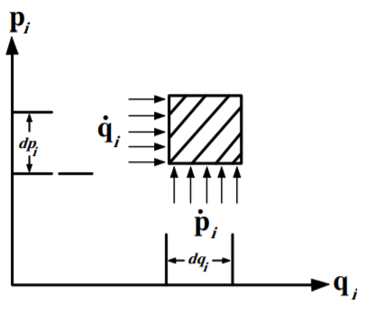
Figure 15.2.1:Infinitessimal element of area in phase space

Consider a density $\rho$ of representative points in $(\mathbf{q}, \mathbf{p})$ phase space. The number $N$ of systems in the volume element $dv$ is

N = \rho dv

where it is assumed that the infinitessimal volume element $dv = dq_1, dq_2....dq_s,dp_1, dp_2....dp_s$ contains many possible systems so that $\rho$ can be considered a continuous distribution. For the conjugate variables $(q_i, p_i)$ shown in Figure 15.2.1, the number of representative points moving across the left-hand edge into the area per unit time is

\rho \dot{q}_i dp_i

The number of representative points flowing out of the area along the right-hand edge is

\left[ \rho \dot{q}_i + \frac{\partial}{ \partial q_i} (\rho \dot{q}_i) dq_i \right] dp_i

Hence the net increase in $\rho$ in the infinitessimal rectangular element $dq_idp_i$ due to flow in the horizontal direction is

− \frac{\partial}{ \partial q_i} (\rho \dot{q}_i) dq_idp_i

Similarly, the net gain due to flow in the vertical direction is

− \frac{\partial}{ \partial p_i} (\rho \dot{p}_i) dp_idq_i

Thus the total increase in the element $dq_idp_i$ per unit time is therefore

− \left[ \frac{\partial}{ \partial q_i } (\rho \dot{q}_i) + \frac{\partial}{ \partial p_i} (\rho \dot{p}_i) \right] dp_idq_i

Assume that the total number of points must be conserved, then the total increase in the number of points inside the element $dq_idp_i$ must equal the net changes in $\rho$ on the infinitessimal surface element per unit time. That is

\left(\frac{\partial \rho}{ \partial t} \right) dq_idp_i

Thus summing over all possible values of $i$ gives

\frac{\partial \rho }{\partial t} + \sum_i \left[ \frac{\partial}{ \partial q_i} (\rho \dot{q}_i) + \frac{\partial}{ \partial p_i} (\rho \dot{p}_i) \right] = 0

\frac{\partial \rho}{ \partial t} +\sum_i \left[ \dot{q}_i \frac{\partial \rho}{ \partial q_i } + \dot{p}_i \frac{\partial \rho}{ \partial p_i} \right] + \rho \sum_i \left[ \frac{\partial \dot{p}_i}{ \partial p_i} + \frac{\partial \dot{q}_i}{ \partial q_i } \right] = 0

Inserting Hamilton’s canonical equations into both brackets and differentiating the last bracket results in

\frac{\partial \rho}{ \partial t} +\sum_i \left[ \frac{\partial H}{ \partial p_i} \frac{\partial \rho }{\partial q_i} − \frac{\partial H}{ \partial q_i} \frac{\partial \rho}{ \partial p_i } \right] + \rho \sum_i \left[\frac{ \partial^2 H}{ \partial p_i\partial q_i} − \frac{\partial^2H}{ \partial p_i\partial q_i} \right] = 0

The two terms in the last bracket cancel and thus

\frac{\partial \rho }{\partial t} +\sum_i \left[ \frac{\partial H }{\partial p_i} \frac{\partial \rho} { \partial q_i} − \frac{\partial H}{ \partial q_i} \frac{\partial \rho}{ \partial p_i} \right] = \frac{\partial \rho}{ \partial t} + \{\rho , H\} = 0

However, this just equals $\frac{d\rho}{ dt}$ , therefore

\frac{d\rho }{dt} = \frac{\partial \rho}{ \partial t} + \{\rho , H\} = 0 \tag{15.70}

This is called Liouville’s theorem which states that the rate of change of density of representative points vanishes, that is, the density of points is a constant in the Hamiltonian phase space along a specific trajectory. Liouville’s theorem means that the system acts like an incompressible fluid that moves such as to occupy an equal volume in phase space at every instant, even though the shape of the phase-space volume may change, that is, the phase-space density of the fluid remains constant. Equation 15.70 is another illustration of the basic Poisson bracket relation 15.45 and the usefulness of Poisson brackets in physics.

Liouville’s theorem is crucially important to statistical mechanics of ensembles where the exact knowledge of the system is unknown, only statistical averages are known. An example is in focussing of beams of charged particles by beam handling systems. At a focus of the beam, the transverse width in $x$ is minimized, while the width in $p_x$ is largest since the beam is converging to the focus, whereas a parallel beam has maximum width $x$ and minimum spreading width $p_x$ . However, the product $xp_x$ remains constant throughout the focussing system. For a two dimensional beam, this applies equally for the $y$ and $p_y$ coordinates, etc. It is obvious that the final beam quality for any beam transport system is ultimately limited by the emittance of the source of the beam, that is, the initial area of the phase space distribution. Note that Liouville’s theorem only applies to Hamiltonian $q_i − p_i$ phase space, not to $x − \dot{x}$ Lagrangian state space. As a consequence, Hamiltonian dynamics, rather than Lagrange dynamics, is used to discuss ensembles in statistical physics.

Note that Liouville’s theorem is applicable only for conservative systems, that is, where Hamilton’s equations of motion apply. For dissipative systems the phase space volume shrinks with time rather than being a constant of the motion.

15.3: Canonical Transformations in Hamiltonian Mechanics¶

Hamiltonian mechanics is an especially elegant and powerful way to derive the equations of motion for complicated systems. Unfortunately, integrating the equations of motion to derive a solution can be a challenge. Hamilton recognized this difficulty, so he proposed using generating functions to make canonical transformations which transform the equations into a known soluble form. Jacobi, a contemporary mathematician, recognized the importance of Hamilton’s pioneering developments in Hamiltonian mechanics, and therefore he developed a sophisticated mathematical framework for exploiting the generating function formalism in order to make the canonical transformations required to solve Hamilton’s equations of motion.

In the Lagrange formulation, transforming coordinates $(q_i, \dot{q}_i)$ to cyclic generalized coordinates $(Q_i, \dot{Q}_i)$ , simplifies finding the Euler-Lagrange equations of motion. For the Hamiltonian formulation, the concept of coordinate transformations is extended to include simultaneous canonical transformation of both the spatial coordinates $q_i$ and the conjugate momenta $p_i$ from $(q_i, p_i)$ to $(Q_i, P_i)$ , where both of the canonical variables are treated equally in the transformation. Compared to Lagrangian mechanics, Hamiltonian mechanics has twice as many variables which is an asset, rather than a liability, since it widens the realm of possible canonical transformations.

Hamiltonian mechanics has the advantage that generating functions can be exploited to make canonical transformations to find solutions, which avoids having to use direct integration. Canonical transformations are the foundation of Hamiltonian mechanics; they underlie Hamilton-Jacobi theory and action-angle variable theory, both of which are powerful means for exploiting Hamiltonian mechanics to solve problems in physics and engineering. The concept underlying canonical transformations is that, if the equations of motion are simplified by using a new set of generalized variables $(\mathbf{Q},\mathbf{P})$ , compared to using the original set of variables $(\mathbf{q},\mathbf{p})$ , then an advantage has been gained. The solution, expressed in terms of the generalized variables $(\mathbf{Q},\mathbf{P})$ , can be transformed back to express the solution in terms of the original coordinates, $(\mathbf{q},\mathbf{p})$ .

Only a specialized subset of transformations will be considered, namely canonical transformations that preserve the canonical form of Hamilton’s equations of motion. That is, given that the original set of variables $(q_i, p_i)$ satisfy Hamilton’s equations

\mathbf{\dot{q}} = \frac{\partial H (\mathbf{q},\mathbf{p}, t)}{ \partial \mathbf{p}} \quad − \mathbf{\dot{p}} = \frac{\partial H (\mathbf{q},\mathbf{p}, t)}{ \partial \mathbf{q}} \tag{15.71}

for some Hamiltonian $H(\mathbf{q},\mathbf{p}, t)$ , then the transformation to coordinates $Q_i(q_k,p_k, t), P_i (q_k, p_k, t)$ is canonical if, and only if, there exists a function $\mathcal{H}(\mathbf{Q},\mathbf{P}, t)$ such that the $\mathbf{ P}$ and $\mathbf{ Q}$ are still governed by Hamilton’s equations. That is,

\mathbf{\dot{Q}} = \frac{\partial\mathcal{H}(\mathbf{Q},\mathbf{P}, t)}{ \partial \mathbf{P}} \quad − \mathbf{\dot{P}} = \frac{\partial\mathcal{H}(\mathbf{Q},\mathbf{P}, t) }{\partial \mathbf{Q}} \tag{15.72}

where $\mathcal{H}(\mathbf{Q},\mathbf{P}, t)$ plays the role of the Hamiltonian for the new variables. Note that $\mathcal{H}(\mathbf{Q},\mathbf{P}, t)$ may be very different from the old Hamiltonian $H(\mathbf{q},\mathbf{p}, t)$ . The invariance of the Poisson bracket to canonical transformations, chapter 15.2, provides a powerful test that the transformation is canonical.

Hamilton’s Principle of least action, discussed in chapter 9, states that

\delta S = \delta \int^{t_2}_{t_1} L(\mathbf{q}, \mathbf{\dot{q}}, t)dt = \delta \int^{t_2}_{t_1} [\mathbf{p} \cdot \mathbf{\dot{q}} − H(\mathbf{q},\mathbf{p}, t)] dt = 0 \tag{15.73}

Similarly, applying Hamilton’s Principle of least action to the new Lagrangian $\mathcal{L}(\mathbf{Q}, \mathbf{\dot{Q}} , t)$ gives

\delta S = \delta \int^{t_2}_{t_1} \mathcal{L}(\mathbf{Q}, \mathbf{\dot{Q}} , t)dt = \delta \int^{t_2}_{t_1} \left[ \mathbf{P} \cdot \mathbf{\dot{Q}} − \mathcal{H}(\mathbf{Q},\mathbf{P}, t) \right] dt = 0 \tag{15.74}

The discussion of gauge-invariant Lagrangians, chapter 9.3, showed that $L$ and $\mathcal{L}$ can be related by the total time derivative of a generating function $F$ where

\frac{dF}{ dt} = \mathcal{L} − L \tag{15.75}

The generating function $F$ can be any well-behaved function with continuous second derivatives of both the old and new canonical variables $\mathbf{p}$ , $\mathbf{q}$ , $\mathbf{P}$ , $\mathbf{Q}$ and $t$ . Thus the integrands of 15.73 and 15.74 are related by

\mathbf{p} \cdot \mathbf{\dot{q}} − H(\mathbf{q},\mathbf{p}, t) = \lambda \left[ \mathbf{P} \cdot \mathbf{\dot{Q}} − \mathcal{H}(\mathbf{Q},\mathbf{P}, t) \right] + \frac{dF}{dt} \tag{15.76}

where $\lambda$ is a possible scale transformation. A scale transformation, such as changing units, is trivial, and will be assumed to be absorbed into the coordinates, making $\lambda = 1$ . Assuming that $\lambda \neq 1$ is called an extended canonical transformation.

Generating functions¶

The generating function $F$ has to be chosen such that the transformation from the initial variables $( \mathbf{q},\mathbf{p})$ to the final variables $(\mathbf{Q},\mathbf{P})$ is a canonical transformation. The chosen generating function contributes to 15.76 only if it is a function of the old plus new variables. The four possible types of generating functions of the first kind, are $F_1(\mathbf{q}, \mathbf{Q}, t)$ , $F_2(\mathbf{q},\mathbf{P}, t)$ , $F_3(\mathbf{p}, \mathbf{Q}, t)$ , and $F_4(\mathbf{p}, \mathbf{P}, t)$ . These four generating functions lead to relatively simple canonical transformations, are shown below.

Type 1: $F = F_1(\mathbf{q}, \mathbf{Q},t)$ :¶

The total time derivative of the generating function $F = F_1(\mathbf{q}, \mathbf{Q},t)$ is given by

\frac{dF(\mathbf{q}, \mathbf{Q},t)}{ dt} = \left[ \frac{\partial F_1(\mathbf{q}, \mathbf{Q},t)}{ \partial \mathbf{q}} \cdot \mathbf{\dot{q}} + \frac{\partial F_1(\mathbf{q}, \mathbf{Q},t)}{ \partial \mathbf{Q}} \cdot \mathbf{\dot{Q}} \right] + \frac{\partial F_1(\mathbf{q}, \mathbf{Q},t) }{\partial t} \tag{15.77}

Insert Equation 15.77 into Equation 15.76, and assume that the trivial scale factor $\lambda = 1$ , then

\left[ \mathbf{p} − \frac{\partial F_1(\mathbf{q}, \mathbf{Q},t)}{ \partial \mathbf{q}} \right] \cdot \mathbf{\dot{q}} − H(\mathbf{q},\mathbf{p}, t) = \left[ \mathbf{P} + \frac{\partial F_1(\mathbf{q}, \mathbf{Q},t)}{ \partial \mathbf{Q}} \right] \cdot \mathbf{\dot{Q}} − \mathcal{H}(\mathbf{Q},\mathbf{P}, t) + \frac{\partial F_1(\mathbf{q}, \mathbf{Q},t) }{\partial t} \nonumber

Assume that the generating function $F_1$ determines the canonical variables $\mathbf{p}$ and $\mathbf{P}$ to be

\mathbf{p} = \frac{\partial F_1(\mathbf{q}, \mathbf{Q},t)}{ \partial \mathbf{q}} \qquad \mathbf{P} = −\frac{\partial F_1(\mathbf{q}, \mathbf{Q},t)}{ \partial \mathbf{Q}} \tag{15.78}

then the terms in each square bracket cancel, leading to the required canonical transformation

\mathcal{H}(\mathbf{Q},\mathbf{P}, t) = H(\mathbf{q},\mathbf{p}, t) + \frac{\partial F_1(\mathbf{q}, \mathbf{Q},t)}{ \partial t} \tag{15.79}

Type 2: $F = F_2(\mathbf{q},\mathbf{P},t) − \mathbf{Q} \cdot \mathbf{P}$ :¶

The total time derivative of the generating function $F = F_2(\mathbf{q},\mathbf{P},t)−\mathbf{Q} \cdot \mathbf{P}$ is given by

\frac{dF}{ dt} = \left[ \frac{\partial F_2(\mathbf{q},\mathbf{P},t)}{ \partial \mathbf{q}} \cdot \mathbf{\dot{q}} + \frac{\partial F_2(\mathbf{q},\mathbf{P},t)}{ \partial \mathbf{P}} \cdot \mathbf{\dot{p}} − \mathbf{P} \cdot \mathbf{\dot{Q}} − \mathbf{\dot{P}} \cdot \mathbf{Q} \right] + \frac{\partial F_2(\mathbf{q},\mathbf{P},t)}{ \partial t} \tag{15.80}

Insert this into Equation 15.76, and assume that the trivial scale factor $\lambda = 1$ , then

\left( \mathbf{p} − \frac{\partial F_2(\mathbf{q},\mathbf{P},t)}{ \partial \mathbf{q}} \right) \cdot \mathbf{\dot{q}} − H(\mathbf{q},\mathbf{p}, t) = \mathbf{P} \cdot \mathbf{\dot{Q}} − \mathbf{P} \cdot \mathbf{\dot{Q}} + \left[ \frac{\partial F_2(\mathbf{q},\mathbf{P},t)}{ \partial \mathbf{P}} − \mathbf{Q} \right] \cdot \mathbf{\dot{P}} − \mathcal{H}(\mathbf{Q},\mathbf{P}, t) + \frac{\partial F_2(\mathbf{q},\mathbf{P},t)}{ \partial t } \nonumber

Assume that the generating function $F_2$ determines the canonical variables $\mathbf{p}$ and $\mathbf{Q}$ to be

\mathbf{p} = \frac{\partial F_2(\mathbf{q},\mathbf{P},t)}{ \partial \mathbf{q}} \qquad \mathbf{Q} = \frac{\partial F_2(\mathbf{q},\mathbf{P},t) }{\partial \mathbf{P}} \tag{15.81}

then the terms in brackets cancel, leading to the required transformation

\mathcal{H}(\mathbf{Q},\mathbf{P}, t) = H(\mathbf{q},\mathbf{p}, t) + \frac{\partial F_2(\mathbf{q},\mathbf{P},t)}{ \partial t} \tag{15.82}

Type 3: $F = F_3(\mathbf{p}, \mathbf{Q},t) + \mathbf{q} \cdot \mathbf{p}$ :¶

The total time derivative of the generating function $F = F_3(\mathbf{p}, \mathbf{Q},t) + \mathbf{q} \cdot \mathbf{p}$ is given by

\frac{dF }{dt} = \left[ \frac{\partial F_3(\mathbf{p}, \mathbf{Q},t)}{ \partial \mathbf{p}} \cdot \mathbf{\dot{p}} + \frac{\partial F_3(\mathbf{p}, \mathbf{Q},t)}{ \partial\mathbf{ Q}} \cdot \mathbf{\dot{Q}} + \mathbf{\dot{q}} \cdot \mathbf{p} + \mathbf{q} \cdot \mathbf{\dot{p}} \right] + \frac{\partial F_3(\mathbf{p}, \mathbf{Q},t)}{ \partial t} \tag{15.83}

Insert this into Equation 15.76, and assume that the trivial scale factor $\lambda = 1$ , then

− \left[ \mathbf{q}+ \frac{\partial F_3(\mathbf{p}, \mathbf{Q},t)}{ \partial \mathbf{p}} \right] \cdot \mathbf{\dot{p}} − H(\mathbf{q},\mathbf{p}, t) = \left[ \mathbf{P}+ \frac{\partial F_3(\mathbf{p}, \mathbf{Q},t)}{ \partial \mathbf{Q}} \right] \cdot \mathbf{\dot{Q}} − \mathcal{H}(\mathbf{Q},\mathbf{P}, t) + \frac{\partial F_3(\mathbf{p}, \mathbf{Q},t)}{ \partial t} \nonumber

Assume that the generating function $F_3$ determines the canonical variables $\mathbf{q}$ and $\mathbf{P}$ to be

\mathbf{q} = −\frac{\partial F_3(\mathbf{p}, \mathbf{Q},t)}{ \partial \mathbf{p}} \qquad \mathbf{P} = −\frac{\partial F_3(\mathbf{p}, \mathbf{Q},t)}{ \partial \mathbf{Q}} \tag{15.84}

then the terms in brackets cancel, leading to the required transformation

\mathcal{H}(\mathbf{Q},\mathbf{P}, t) = H(\mathbf{q},\mathbf{p}, t) + \frac{\partial F_3(\mathbf{p}, \mathbf{Q},t)}{ \partial t} \tag{15.85}

Type 4: $F = F_4(\mathbf{p}, \mathbf{P},t) + \mathbf{q} \cdot \mathbf{p} − \mathbf{Q} \cdot \mathbf{P}$ :¶

The total time derivative of the generating function $F = F_4(\mathbf{p}, \mathbf{P},t) + \mathbf{q} \cdot \mathbf{p} − \mathbf{Q} \cdot \mathbf{P}$ is given by

\frac{dF }{dt} = \left[ \frac{\partial F_4(\mathbf{p}, \mathbf{P},t)}{ \partial \mathbf{p}} \cdot \mathbf{\dot{p}} + \frac{\partial F_4(\mathbf{p}, \mathbf{P},t) }{\partial \mathbf{P}} \cdot \mathbf{\dot{p}} + \mathbf{\dot{q}} \cdot \mathbf{p} + \mathbf{q} \cdot \mathbf{\dot{p}} − \mathbf{\dot{Q}} \cdot \mathbf{P} − \mathbf{Q} \cdot \mathbf{\dot{P}} \right] + \frac{\partial F_4(\mathbf{p}, \mathbf{P},t)}{ \partial t}\tag{15.86}

Insert this into Equation 15.76, and assume that the trivial scale factor $\lambda = 1$ , then

− \left[ \mathbf{q}+ \frac{\partial F_4(\mathbf{p}, \mathbf{P},t)}{ \partial \mathbf{p}} \right] \cdot \mathbf{\dot{p}} − H(\mathbf{q},\mathbf{p}, t) = \left[ \frac{\partial F_4(\mathbf{p}, \mathbf{P},t)}{ \partial \mathbf{P} } − \mathbf{Q} \right] \cdot \mathbf{\dot{P}} − \mathcal{H}(\mathbf{Q},\mathbf{P}, t) + \frac{\partial F_4(\mathbf{p}, \mathbf{P},t) }{\partial t} \nonumber

Assume that the generating function $F_4$ determines the canonical variables $\mathbf{q}$ and $\mathbf{Q}$ to be

\mathbf{q} = −\frac{\partial F_4(\mathbf{p}, \mathbf{P},t)}{ \partial \mathbf{p}} \qquad \mathbf{Q} = \frac{\partial F_4(\mathbf{p}, \mathbf{P},t)}{ \partial \mathbf{P}} \tag{15.87}

then the terms in brackets cancel, leading to the required transformation

\mathcal{H}(\mathbf{Q},\mathbf{P}, t) = H(\mathbf{q},\mathbf{p}, t) + \frac{\partial F_4(\mathbf{p}, \mathbf{P},t)}{ \partial t} \tag{15.88}

Note that the last three generating functions require the inclusion of additional bilinear products of $q$ , $p$ , $Q$ , $P$ in order for the terms to cancel to give the required result. The addition of the bilinear terms, ensures that the resultant generating function $F$ is the same using any of the four generating functions $F_1$ , $F_2$ , $F_3$ , $F_4$ . Frequently the $F_2(\mathbf{q},\mathbf{P}, t)$ generating function is the most convenient. The four possible generating functions of the first kind, given above, are related by Legendre transformations. A canonical transformation does not have to conform to only one of the four generating functions $F_k$ for all the degrees of freedom, they can be a mixture of different flavors for the different degrees of freedom. The properties of the generating functions are summarized in table 15.3.1.

Generating function	Generating function derivatives	Trivial special examples
$F = F_1(\mathbf{q}, \mathbf{Q}, t)$	$p_i = \frac{\partial F_1}{ \partial q_i } \quad P_i = −\frac{\partial F_1}{ \partial Q_i}$	$F_1 = q_iQ_i \quad Q_i = p_i \quad P_i = −q_i$
$F = F_2(\mathbf{q},\mathbf{P}, t) − \mathbf{Q} \cdot \mathbf{P}$	$p_i = \frac{\partial F_2}{ \partial q_i} \quad Q_i = \frac{\partial F_2}{ \partial P_i}$	$F_2 = q_iP_i \quad Q_i = q_i \quad P_i = p_i$
$F = F_3(\mathbf{p}, \mathbf{Q},t) + \mathbf{q} \cdot \mathbf{p}$	$q_i = −\frac{\partial F_3}{ \partial p_i} \quad P_i = −\frac{\partial F_3}{ \partial Q_i}$	$F_3 = p_iQ_i \quad Q_i = −q_i \quad P_i = −p_i$
$F = F_4(\mathbf{p},\mathbf{P},t) + \mathbf{q} \cdot \mathbf{p} − \mathbf{Q} \cdot \mathbf{P}$	$q_i = −\frac{\partial F_4}{ \partial p_i } \quad Q_i = \frac{\partial F_4}{ \partial P_i}$	$F_4 = p_iP_i \quad Q_i = p_i \quad P_i = −q_i$

The partial derivatives of the generating functions $F_i$ determine the corresponding conjugate variables not explicitly included in the generating function $F_i$ . Note that, for the first trivial example $F_1 = q_iQ_i$ , the old momenta become the new coordinates, $Q_i = p_i$ , and vice versa, $P_i = −q_i$ . This illustrates that it is better to name them “conjugate variables” rather than “momenta” and “coordinates”.

In summary, Jacobi has developed a mathematical framework for finding the generating function $F$ required to make a canonical transformation to a new Hamiltonian $\mathcal{H}(\mathbf{Q},\mathbf{P}, t)$ , that has a known solution. That is,

\mathcal{H}(\mathbf{Q},\mathbf{P}, t) = H(\mathbf{q},\mathbf{p}, t) + \frac{\partial F}{ \partial t} \tag{15.89}

When $\mathcal{H}(\mathbf{Q},\mathbf{P}, t)$ is a constant, then a solution has been obtained. The inverse transformation for this solution $\mathbf{Q}(t), \mathbf{P}(t) \rightarrow \mathbf{q}(t), \mathbf{p}(t)$ now can be used to express the final solution in terms of the original variables of the system.

Note the special case when $\mathcal{H}(\mathbf{Q},\mathbf{P}, t)=0$ , then Equation 15.89 has been reduced to the Hamilton-Jacobi relation 15.11

H(\mathbf{q},\mathbf{p}, t) + \frac{\partial S}{\partial t} = 0 \tag{15.11}

In this case, the generating function $F$ determines the action functional $S$ required to solve the Hamilton-Jacobi equation $(15.4.23)$ ). Since Equation 15.89 has transformed the Hamiltonian $H(\mathbf{q},\mathbf{p}, t) \rightarrow \mathcal{H}(\mathbf{Q},\mathbf{P}, t)$ , for which $\mathcal{H}(\mathbf{Q},\mathbf{P}, t)=0$ , then the solution $\mathbf{Q}(t), \mathbf{P}(t)$ for the Hamiltonian $\mathcal{H}(\mathbf{Q},\mathbf{P}, t)=0$ is obtained easily. This approach underlies Hamilton-Jacobi theory presented in chapter 15.4.

Applications of Canonical Transformations¶

The canonical transformation procedure may appear unnecessarily complicated for solving the examples given in this book, but it is essential for solving the complicated systems that occur in nature. For example, canonical transformations can be used to transform time-dependent, (non-autonomous) Hamiltonians to time-independent, (autonomous) Hamiltonians for which the solutions are known. Example 15.6.2 describes such a system. Canonical transformations provide a remarkably powerful approach for solving the equations of motion in Hamiltonian mechanics, especially when using the Hamilton-Jacobi approach discussed in chapter 15.4.

Example 15.3.4: Infinitessimal point canonical transformation

Consider an infinitessimal point canonical transformation, that is infinitesimally close to a point identity.

F_2(\mathbf{q} \cdot \mathbf{P},t) = \mathbf{q} \cdot \mathbf{P}+\epsilon G (\mathbf{q},\mathbf{P},t) \nonumber

satisfies 15.89 if the following relations are satisfied

Q_i = \frac{\partial F_2}{ \partial P_i} = q_i + \epsilon \frac{\partial G(\mathbf{q},\mathbf{P}, t) }{\partial P_i} \nonumber

p_i = \frac{\partial F_2 }{\partial q_i} = P_i + \epsilon \frac{\partial G(\mathbf{q},\mathbf{P}, t)}{ \partial q_i} \nonumber

Thus the infinitessimal changes in $q_i$ and $p_i$ are given by

\delta q_i(\mathbf{q},\mathbf{p},t) = Q_i − q_i = \epsilon \frac{\partial G(\mathbf{q},\mathbf{P}, t)}{ \partial P_i } = \epsilon \frac{\partial G(\mathbf{q},\mathbf{P}, t)}{ \partial p_i} + O(\epsilon^2) \nonumber

\delta p_i(\mathbf{q},\mathbf{p},t) = P_i − p_i = −\epsilon \frac{\partial G(\mathbf{q},\mathbf{P}, t)}{ \partial q_i} = −\epsilon \frac{\partial G(\mathbf{q},\mathbf{P}, t)}{ \partial p_i} + O(\epsilon^2) \nonumber

Thus $G(\mathbf{q},\mathbf{P},t)$ is the generator of the infinitessimal canonical transformation.

Example 15.3.5: 1-D harmonic oscillator via a cononical transformation

The classic one-dimensional harmonic oscillator provides an example of the use of canonical transformations. Consider the Hamiltonian where $\omega^2 = \frac{k}{m}$ then

H = \frac{p^2}{2m} + \frac{kq^2}{ 2} = \frac{1}{ 2m} \left( p^2 + m^2\omega^2q^2\right) \nonumber

This form of the Hamiltonian is a sum of two squares suggesting a canonical transformation for which $H$ is cyclic in a new coordinate. A guess for a canonical transformation is of the form $p = m\omega q \cot Q$ which is of the $F_1(\mathbf{q}, \mathbf{Q})$ type where $F_1$ equals $F_1(\mathbf{q}, \mathbf{Q}) = \frac{m\omega q^2}{2} \cot Q$ . Using 15.78 gives

p = \frac{\partial F_1(q,Q) }{\partial q_i} = m\omega q \cot Q \nonumber

P = −\frac{\partial F_1(q, Q)}{ \partial Q} = \frac{m}{ 2} \frac{\omega q^2}{ \sin^2 Q} \nonumber

Solving for the coordinates $(p, q)$ yields

q = \sqrt{\frac{2P}{ m\omega}} \sin Q \tag{a}

p = \sqrt{2m\omega P} \cos Q \tag{b}

Inserting these into $H$ gives

\mathcal{H} =\omega P(\cos^2 Q + \sin^2 Q) = \omega P \nonumber

which implies that $Q$ is a cyclic coordinate.

The Hamiltonian is conservative, since it does not explicitly depend on time, and it equals the total energy since the transformation to generalized coordinates is time independent. Thus

\mathcal{H} =E = \omega P \nonumber

Since

\dot{Q} = \frac{\partial \mathcal{H}}{ \partial P} = \omega \nonumber

then

Q = \omega t + \phi \nonumber

Substituting $Q$ into a gives the well known solution of the one-dimensional harmonic oscillator

q = \sqrt{\frac{2E}{ m\omega^2}} \sin (\omega t + \phi ) \nonumber

15.4: Hamilton-Jacobi Theory¶

Hamilton used the Principle of Least Action to derive the Hamilton-Jacobi relation (chapter 15.3)

H(\mathbf{q},\mathbf{p}, t) + \frac{\partial S}{\partial t} = 0 \tag{15.11}

where $\mathbf{q}, \mathbf{p}$ refer to the $1 \leq i \leq n$ variables $q_i, p_i$ and $S(q_j (t_1), t_1, q_j (t_2), t_2)$ is the action functional. Integration of this first-order partial differential equation is non trivial which is a major handicap for practical exploitation of the Hamilton-Jacobi equation. This stimulated Jacobi to develop the mathematical framework for canonical transformation that are required to solve the Hamilton-Jacobi equation. Jacobi’s approach is to exploit generating functions for making a canonical transformation to a new Hamiltonian $\mathcal{H}(\mathbf{Q}, \mathbf{P}, t)$ that equals zero.

\mathcal{H}(\mathbf{Q},\mathbf{P}, t) = H(\mathbf{q},\mathbf{p}, t) + \frac{\partial S}{\partial t} = 0 \tag{15.90}

The generating function for solving the Hamilton-Jacobi equation then equals the action functional $S$ .

The Hamilton-Jacobi theory is based on selecting a canonical transformation to new coordinates $(Q, P, t)$ all of which are either constant, or the $Q_i$ are cyclic, which implies that the corresponding momenta $P_i$ are constants. In either case, a solution to the equations of motion is obtained. A remarkable feature of Hamilton-Jacobi theory is that the canonical transformation is completely characterized by a single generating function, $S$ . The canonical equations likewise are characterized by a single Hamiltonian function, $H$ . Moreover, the generating function $S$ , and Hamiltonian function $H$ , are linked together by Equation 15.11. The underlying goal of Hamilton-Jacobi theory is to transform the Hamiltonian to a known form such that the canonical equations become directly integrable. Since this transformation depends on a single scalar function, the problem is reduced to solving a single partial differential equation.

Time-dependent Hamiltonian¶

Jacobi’s complete integral $S(q_i, P_i, t)$ ¶

The principle underlying Jacobi’s approach to Hamilton-Jacobi theory is to provide a recipe for finding the generating function $F = S$ needed to transform the Hamiltonian $H(\mathbf{q}, \mathbf{p}, t)$ to the new Hamiltonian $\mathcal{H}(\mathbf{Q}, \mathbf{P}, t)$ using Equation 15.90. When the derivatives of the transformed Hamiltonian $\mathcal{H}(\mathbf{Q}, \mathbf{P}, t)$ are zero, then the equations of motion become

\dot{Q}_i = \frac{\partial \mathcal{H}}{ \partial P_i} = 0 \tag{15.91}

\dot{P}_i = − \frac{\partial \mathcal{H}}{ \partial Q_i } = 0 \tag{15.92}

and thus $Q_i$ and $P_i$ are constants of motion. The new Hamiltonian $\mathcal{H}$ must be related to the original Hamiltonian $H$ by a canonical transformation for which

\mathcal{H}(\mathbf{Q}, \mathbf{P}, t) = H(\mathbf{q}, \mathbf{p}, t) + \frac{\partial S}{ \partial t} \tag{15.93}

Equations 15.91 and 15.92 are automatically satisfied if the new Hamiltonian $\mathcal{H} = 0$ since then Equation 15.93 gives that the generating function $S$ satisfies Equation 15.90.

Any of the four types of generating function can be used. Jacobi chose the type 2 generating function as being the most useful for many practical cases, that is, $S(q_i, P_i, t)$ which is called Jacobi’s complete integral.

For generating functions $F_1$ and $F_2$ the generalized momenta are derived from the action by the derivative

p_i = \frac{\partial S}{ \partial q_i} \tag{15.4}

Use this generalized momentum to replace $p_i$ in the Hamiltonian $H$ , given in Equation 15.93, leads to the Hamilton-Jacobi equation expressed in terms of the action $S$ .

H(q_1, ...q_n; \frac{\partial S}{ \partial q_1 }, ..., \frac{\partial S}{ \partial q_n} ;t) + \frac{\partial S}{ \partial t} = 0 \tag{15.94}

The Hamilton-Jacobi equation, 15.94, can be written more compactly using tensors $\mathbf{q}$ and $\boldsymbol{\nabla}S$ to designate $(q_1, ..q_n)$ and $\frac{\partial S}{ \partial q_1 }, ..., \frac{\partial S}{ \partial q_n}$ respectively. That is

H(\mathbf{q}, \boldsymbol{\nabla}S, t) + \frac{\partial S}{\partial t} = 0 \tag{15.95}

Equation 15.95 is a first-order partial differential equation in $n + 1$ variables which are the old spatial coordinates $q_i$ plus time $t$ . The new momenta $P_i$ have not been specified except that they are constants since $\mathcal{H} = 0$ .

Assume the existence of a solution of 15.95 of the form $S(q_i, P_i, t) = S(q_1, ..q_n; \alpha_1, ..\alpha_{n+1};t)$ where the generalized momenta $P_i = \alpha_1, \alpha_2, ....\alpha$ plus $t$ are the $n + 1$ independent constants of integration in the transformed frame. One constant of integration is irrelevant to the solution since only partial derivatives of $S(q_i, P_i, t)$ with respect to $q_i$ and $t$ are involved. Thus, if $S$ is a solution of the first-order partial differential equation, then so is $S + \alpha$ where $\alpha$ is a constant. Thus it can be assumed that one of the $n + 1$ constants of integration is just an additive constant which can be ignored leading effectively to a solution

S(q_i, P_i, t) = S(q_1, .....q_n;\alpha_1, .....\alpha_n;t) \tag{15.96}

where none of the $n$ independent constants are solely additive. Such generating function solutions are called complete solutions of the first-order partial differential equations since all constants of integration are known.

It is possible to assume that the $n$ generalized momenta, $P_i$ are constants $\alpha_i$ , where the $\alpha_i$ are the constants. This allows the generalized momentum to be written as

p_i = \frac{\partial S(\mathbf{q}, \boldsymbol{\alpha}, t)}{ \partial q_i } \tag{15.97}

Similarly, Hamilton’s equations of motion give the conjugate coordinate $\mathbf{Q} = \boldsymbol{\beta}$ , where $\beta_i$ are constants. That is

Q_i = \beta_i = \frac{\partial S(\mathbf{q}, \boldsymbol{\alpha}, t)}{ \partial \alpha_i} \tag{15.98}

The above procedure has determined the complete set of $2n$ constants $(\mathbf{Q} = \boldsymbol{\beta}, \mathbf{P} = \boldsymbol{\alpha})$ . It is possible to invert the canonical transformation to express the above solution, which is expressed in terms of $Q_i = \beta_i$ and $P_i = \alpha_i$ , back to the original coordinates, that is, $q_j = q_j (\alpha , \beta , t)$ and momenta $p_j = p_j (\alpha , \beta , t)$ which is the required solution.

Hamilton’s principle function $S_H(\mathbf{q}_i, t; \mathbf{q}_o t_o)$ ¶

Hamilton’s approach to solving the Hamilton-Jacobi Equation 15.95 is to seek a canonical transformation from variables $(\mathbf{p}, \mathbf{q})$ at time $t$ , to a new set of constant quantities, which may be the initial values $(\mathbf{q}_0, \mathbf{p}_0)$ at time $t = 0$ . Hamilton’s principle function $S_H(q_i, t; q_ot_o)$ is the generating function for this canonical transformation from the variables $(\mathbf{q}, \mathbf{p})$ at time t to the initial variables $(\mathbf{q}_0, \mathbf{p}_0)$ at time $t_0$ . Hamilton’s principle function $S_H(q_i, t; q_ot_o)$ is directly related to Jacobi’s complete integral $S(q_i, P_i, t)$ .

Note that $S_H$ is the generating function of a canonical transformation from the present time $(\mathbf{q}, \mathbf{p}, t)$ variables to the initial $(\mathbf{q}_0, \mathbf{p}_0, t_0)$ , whereas Jacobi’s $S$ is the generating function of a canonical transformation from the present $(\mathbf{q},\mathbf{p}, t)$ variables to the constant variables $(\mathbf{Q} = \boldsymbol{\beta}, \mathbf{P} = \boldsymbol{\alpha})$ . For the Hamilton approach, the canonical transformation can be accomplished in two steps using $S$ by first transforming from $(\mathbf{q}, \mathbf{p}, t)$ at time $t$ , to $(\boldsymbol{\beta}, \boldsymbol{\alpha})$ , then transforming from $(\boldsymbol{\beta}, \boldsymbol{\alpha})$ to $(\mathbf{q}_0,\mathbf{p}_0, t_0)$ . That is, this two-step process corresponds to

S_H(\mathbf{q}, t; \mathbf{q}_ot_o) = S(\mathbf{q}, \boldsymbol{\alpha}, t) − S(\mathbf{q}_0, \boldsymbol{\alpha}, t_0) \tag{15.99}

Hamilton’s principle function $S_H(\mathbf{q}, t; \mathbf{q}_ot_o)$ is related to Jacobi’s complete integral $S(\mathbf{q}, \boldsymbol{\alpha}, t)$ , and it will not be discussed further in this book.

Time-independent Hamiltonian¶

Frequently the Hamiltonian does not explicitly depend on time. For the standard Lagrangian with time-independent constraints and transformation, then $H (\mathbf{q}, \mathbf{p},t) = E$ which is the total energy. For this case, the Hamilton-Jacobi equation simplifies to give

\frac{\partial S}{ \partial t} = −H( \mathbf{ q}, \mathbf{ p}, t) = −E (\boldsymbol{\alpha}) \tag{15.100}

The integration of the time dependence is trivial, and thus the action integral for a time-independent Hamiltonian equals

S(\mathbf{q}, \boldsymbol{\alpha},t) = W (\mathbf{q}, \boldsymbol{\alpha}) − E (\boldsymbol{\alpha})t \tag{15.101}

That is, the action integral has separated into a time independent term $W (\mathbf{q}, \boldsymbol{\alpha})$ which is called Hamilton’s characteristic function plus a time-dependent term $−E (\boldsymbol{\alpha})t$ . Thus using equations 15.97, 15.101 gives that the generalized momentum is

p_i = \frac{\partial W(\mathbf{q}, \boldsymbol{\alpha})}{ \partial q_i} \tag{15.102}

The physical significance of Hamilton’s characteristic function $W (\mathbf{q}, \boldsymbol{\alpha})$ can be understood by taking the total time derivative

\frac{dW}{ dt} = \sum_i \frac{\partial W(\mathbf{q}, \boldsymbol{\alpha})}{ \partial q_i} \dot{q}_i = \sum_i p_i\dot{q}_i \nonumber

Taking the time integral then gives

W (\mathbf{q}, \boldsymbol{\alpha}) = \int \sum p_i\dot{q}_i dt =\int \sum p_idq_i \tag{15.103}

Note that this equals the abbreviated action described in chapter 9.2.3, that is $W(\mathbf{q}, \boldsymbol{\alpha}) = S_0(\mathbf{q}, \boldsymbol{\alpha})$ .

Inserting the action $S (\mathbf{q}, \boldsymbol{\alpha})$ into the Hamilton-Jacobi equation $(15.2.1)$ gives

H(\mathbf{q}; \frac{\partial W(\mathbf{q}, \boldsymbol{\alpha})}{ \partial \mathbf{q}} ) = E (\boldsymbol{\alpha}) \tag{15.104}

This is called the time-independent Hamilton-Jacobi equation. Usually it is convenient to have $E$ equal the total energy. However, sometimes it is more convenient to exclude the $k^{th}$ energy $E(\alpha_k)$ in the set, in which case $E = E(\alpha_1, \alpha_2, ...\alpha_k−1)$ ; the Routhian exploits this feature.

The equations of the canonical transformation expressed in terms of $W (\mathbf{q}, \boldsymbol{\alpha})$ are

p_i = \frac{\partial W(\mathbf{q}, \boldsymbol{\alpha}) }{\partial q_i } \quad \beta_i + \frac{\partial E(\boldsymbol{\alpha}) }{\partial \alpha_i} t = \frac{\partial W(\mathbf{q}, \boldsymbol{\alpha})}{ \partial \alpha_i} \tag{15.105}

These equations show that Hamilton’s characteristic function $W (\mathbf{q}, \boldsymbol{\alpha})$ is itself the generating function of a time-independent canonical transformation from the old variables $(q, p)$ to a set of new variables

Q_i = \beta_i + \frac{\partial E(\boldsymbol{\alpha})}{ \partial \alpha_i } t \quad P_i = \alpha_i \tag{15.106}

Table 15.4.1 summarizes the time-dependent and time-independent forms of the Hamilton-Jacobi equation.

Hamiltonian	Time dependent $H(q, p, t)$	Time independent $H(q, p)$
Transformed Hamiltonian	$\mathcal{H}= 0$	$\mathcal{H}$ is cyclic
Canonical transformed variables	All $Q_iP_i$ are constants of motion	All $P_i$ are constants of motion
Transformed equations of motion	$\dot{Q}_i = \frac{\partial \mathcal{H}}{ \partial P_i} = 0$ , therefore $Q_i = \beta_i$ $\dot{P}_i = − \frac{\partial \mathcal{H}}{ \partial Q_i} = 0$ , therefore $P_i = \alpha_i$	$\dot{Q}_i = \frac{\partial \mathcal{H}}{ \partial P_i} = v_i$ , therefore $Q_i = v_i t + \beta_i$ $\dot{P}_i = − \frac{\partial \mathcal{H}} {\partial Q_i} = 0$ , therefore $P_i = \alpha_i$
Generating function	Jacobi’s complete integral $S(\mathbf{q}, \mathbf{P}, t)$	Characteristic Function $W(\mathbf{q}, \mathbf{P})$
Hamilton-Jacobi equation	$H(q_1, ...q_n; \frac{\partial S}{ \partial q_1 }, ..., \frac{\partial S} {\partial q_n} ;t)+\frac{\partial S}{ \partial t} = 0$	$H(q_1, ...q_n; \frac{\partial W }{\partial q_1} , ..., \frac{\partial W}{ \partial q_n} ) = E$
Transformation equations	$p_i= \frac{\partial S}{ \partial q_i}$ $Q_i= \frac{\partial S}{ \partial \alpha_i} = \beta_i$	$p_i=\frac{\partial W}{ \partial q_i}$ $Q_i=\frac{\partial W}{ \partial \alpha_i} = v_i t + \beta_i$

Separation of variables¶

Exploitation of the Hamilton-Jacobi theory requires finding a suitable action function $S$ . When the Hamiltonian is time independent, then Equation 15.101 shows that the time dependence of the action integral separates out from the dependence on the spatial variables. For many systems, the Hamilton’s characteristic function $W(\mathbf{q}, \mathbf{P})$ separates into a simple sum of terms each of which is a function of a single variable. That is,

W(\mathbf{q}, \boldsymbol{\alpha}) = W_1(q_1) + W_2(q_2) + \cdots \cdot \cdot W_n(q_n) \tag{15.107}

where each function in the summation on the right depends only on a single variable. Then Equation 15.100 reduces to

H(q_1, ...q_n; \frac{\partial W }{\partial q_1} , ...,\frac{ \partial W}{ \partial q_n} ) = E \tag{15.108}

where $E$ is the constant denoting the total energy.

Hamilton’s characteristic function $W( \mathbf{ q}, \mathbf{ P})$ can be used with equations 15.101, 15.102, 15.91, 15.92, and 15.93 to derive

p_i = \frac{\partial W( \mathbf{ q}, \boldsymbol{\alpha}) }{\partial q_i} \quad Q_i = \frac{\partial W( \mathbf{ q}, \boldsymbol{\alpha}) }{\partial P_i} \tag{15.109}

\dot{Q}_i = \frac{\partial \mathcal{H}}{ \partial P_i} = 0 \quad \dot{P}_i = \frac{\partial \mathcal{H}}{ \partial Q_i} = 0 \tag{15.110}

\mathcal{H} = H + \frac{\partial S}{\partial t} = H − E = 0 \tag{15.111}

which has reduced the problem to a simple sum of one-dimensional first-order differential equations.

If the $i^{th}$ variable is cyclic, then the Hamiltonian is not a function of $q_i$ and the $i^{th}$ term in Hamilton’s characteristic function equals $W_i = \alpha_iq_i$ which separates out from the summation in Equation 15.107. That is, all cyclic variables can be factored out of $W( \mathbf{ q}, \boldsymbol{\alpha})$ which greatly simplifies solution of the Hamilton-Jacobi equation. As a consequence, the ability of the Hamilton-Jacobi method to make a canonical transformation to separate the system into many cyclic or independent variables, which can be solved trivially, is a remarkably powerful way for solving the equations of motion in Hamiltonian mechanics.

Example 15.4.1: Free particle

Consider the motion of a free particle of mass $m$ in a force-free region. Then Equation 15.93 reduces to

H(q_1, ...q_n; \frac{\partial S}{ \partial q_1} , ..., \frac{\partial S}{ \partial q_n} ;t) + \frac{\partial S}{\partial t} = 0 \nonumber

Since no forces act, and the momentum $\mathbf{p} = \boldsymbol{\nabla}S$ , thus the Hamilton-Jacobi equation reduces to

\frac{1}{ 2m } \nabla^2S + \frac{\partial S}{\partial t} = 0 \tag{A}

The Hamiltonian is time independent, thus Equation 15.101 applies

S(\mathbf{q}, t) = W(\mathbf{q}, \boldsymbol{\alpha}) − E(\boldsymbol{\alpha})t \nonumber

Since the Hamiltonian does not explicitly depend on the coordinates $(x, y, z)$ , then the coordinates are cyclic and separation of the variables, 15.107, gives that the action

S = \boldsymbol{\alpha} \cdot \mathbf{ r} − Et \tag{B}

For Equation B to be a solution of Equation A requires that

E = \frac{1}{ 2m} \boldsymbol{\alpha}^2 \tag{C}

Therefore

S = \boldsymbol{\alpha} \cdot \mathbf{r} − \frac{1}{ 2m} \boldsymbol{\alpha}^2t \tag{D}

Since

\mathbf{\dot{Q}} = \frac{\partial S }{\partial \boldsymbol{\alpha} } = \mathbf{r}− \frac{\boldsymbol{\alpha}}{ m }t \nonumber

the equation of motion and the conjugate momentum are given by

\mathbf{r} = \mathbf{\dot{Q}} + \frac{\boldsymbol{\alpha}}{ m} t \quad \mathbf{p} = \boldsymbol{\nabla}S = \boldsymbol{\alpha} \nonumber

Thus the Hamilton-Jacobi relation has given both the equation of motion and the linear momentum $\mathbf{p}$ .

Example 15.4.2: Point particle in a uniform gravitational field

The Hamiltonian is

H = \frac{1}{ 2m} (p^2_x + p^2_y + p^2_z) + mgz \nonumber

Since the system is conservative, then the Hamilton-Jacobi equation can be written in terms of Hamilton’s characteristic function $W$

E = \frac{1}{ 2m} \left[\left(\frac{\partial W}{ \partial x} \right)^2 + \left(\frac{\partial W}{ \partial y} \right)^2 + \left(\frac{\partial W}{ \partial z} \right)^2 \right] + mgz \nonumber

Assuming that the variables can be separated $W = X(x) + Y (y) + Z(z)$ leads to

p_x = \frac{\partial X(x)}{ \partial x} = \alpha_x \nonumber

p_y = \frac{\partial Y (y)}{ \partial y} = \alpha_y \nonumber

p_z = \frac{\partial Z(z) }{\partial z} = \sqrt{ 2m(E − mgz) − \alpha^2_x − \alpha^2_y} \nonumber

Thus by integration the total $W$ equals

W = \int^x_{x_0} \alpha_x dx + \int^y_{y_0} \alpha_ydy + \int^z_{z_0} \left(\sqrt{ 2m(E − mgz) − \alpha^2_x − \alpha^2_y }\right) dz \nonumber

Therefore using 15.106 gives

\beta_z = t − t_0 = \int^z_{z_0} \frac{mdz}{ \sqrt{ 2m(E − mgz) − \alpha^2_x − \alpha^2_y } } \nonumber

\beta_x = \text{ constant }= (x − x_0) − \int^z_{z_0} \frac{\alpha_xdz}{ \sqrt{ 2m(E − mgz) − \alpha^2_x − \alpha^2_y } } \nonumber

\beta_y = \text{ constant } = (y − y_0) − \int^z_{z_0} \frac{\alpha_ydz }{\sqrt{ 2m(E − mgz) − \alpha^2_x − \alpha^2_y }} \nonumber

If $x_0, y_0, z_0$ is the position of the particle at time $t = t_0$ then $\beta_x = \beta_y = 0$ , and from 15.106

x − x_0 = \left(\frac{\alpha_x}{ m }\right) (t − t_0) \nonumber

y − y_0 = \left(\frac{\alpha_y}{ m} \right) (t − t_0) \nonumber

z − z_0 = \left( \frac{\sqrt{ 2m(E − mgz) − \alpha^2_x − \alpha^2_y }}{ m} \right) (t − t_0) − \frac{1}{ 2} g(t − t_0)^2 \nonumber

This corresponds to a parabola as should be expected for this trivial example.

Example 15.4.3: One-dimensional harmonic oscillator

As discussed in example 15.3.5 the Hamiltonian for the one-dimensional harmonic oscillator can be written as

H = \frac{1}{ 2m} ( p^2 + m^2\omega^2q^2) = E \nonumber

assuming it is conservative and where $\omega = \sqrt{\frac{k}{m}}$ .

Hamilton’s characteristic function $W$ can be used where

S (q, E, t) = W (q, E) − Et \nonumber

p_i = \frac{\partial W}{ \partial q_i} \nonumber

Inserting the generalized momentum $p_i$ into the Hamiltonian gives

\frac{1}{ 2m} \left(\left[ \frac{\partial W }{\partial q} \right]^2 + m^2\omega^2q^2 \right) = E \nonumber

Integration of this equation gives

W = \sqrt{ 2mE} \int dq \sqrt{1 − \frac{m\omega^2q^2}{ 2E}} \nonumber

That is

S = \sqrt{ 2mE } \int dq \sqrt{ 1 − \frac{m\omega^2q^2}{ 2E}} − Et \nonumber

Note that

\frac{\partial S(q, E, t)}{ \partial E} = \sqrt{\frac{2m }{E}} \int \frac{dq}{\sqrt{1 - \frac{ m\omega^2q^2}{ 2E}}} − t \nonumber

This can be integrated to give

t = \frac{1}{ \omega }\arcsin \left( q \sqrt{\frac{m\omega^2}{ 2E}}\right) + t_0 \nonumber

That is

q = \sqrt{\frac{2E}{m\omega^2}} \sin \omega (t − t_0) \nonumber

This is the familiar solution of the undamped harmonic oscillator.

Example 15.4.4: The central force problem

The problem of a particle acted upon by a central force occurs frequently in physics. Consider the mass $m$ acted upon by a time-independent central potential energy $U(r)$ . The Hamiltonian is time independent and can be written in spherical coordinates as

H = \frac{1}{ 2m} \left( p^2_r + \frac{1}{r^2} p^2_{\theta} + \frac{1}{r^2 \sin^2 \theta} p^2_{\psi} \right) + U(r) = E \nonumber

The time-independent Hamilton-Jacobi equation is conservative, thus

\frac{1}{ 2m} \left[\left(\frac{\partial W}{ \partial r }\right)^2 + \frac{1}{ r^2} \left(\frac{\partial W }{\partial \theta} \right)^2 + \frac{1}{ r^2 \sin^2 \theta} \left(\frac{\partial W}{ \partial \phi} \right)^2 \right] + U(r) = E \nonumber

Try a separable solution for Hamilton’s characteristic function $W$ of the form

W = R(r) + \Theta (\theta ) + \Phi (\phi ) \nonumber

The Hamilton-Jacobi equation then becomes

\frac{1}{ 2m} \left[\left(\frac{\partial R} {\partial r} \right)^2 + \frac{1}{ r^2} \left(\frac{\partial \Theta}{ \partial \theta} \right)^2 + \frac{1}{ r^2 \sin^2 \theta} \left(\frac{\partial \Phi}{ \partial \phi } \right)^2 \right] + U(r) = E \nonumber

This can be rearranged into the form

2mr^2 \sin^2 \theta \left\{ \frac{1}{ 2m} \left[\left(\frac{\partial R}{ \partial r} \right)^2 + \frac{1} {r^2} \left(\frac{\partial \Theta}{ \partial \theta} \right)^2 \right] + U(r) + E \right\} = − \left(\frac{\partial \Phi}{ \partial \phi} \right)^2 \nonumber

The left-hand side is independent of $\phi$ whereas the right-hand side is independent of $r$ and $\theta$ . Both sides must equal a constant which is set to equal $−L^2_z$ , that is

\frac{1}{2m} \left[\left(\frac{\partial R}{ \partial r} \right)^2 + \frac{1}{ r^2} \left(\frac{\partial \Theta}{ \partial \theta} \right)^2 \right] + U(r) + \frac{L^2_z }{2mr^2 \sin^2 \theta} = E \nonumber

\left(\frac{\partial \Phi}{ \partial \phi} \right)^2 = L^2_z \nonumber

The equation in $r$ and $\theta$ can be rearranged in the form

2mr^2 \left[ \frac{1}{2m} \left(\frac{\partial R}{ \partial r} \right)^2 + U(r) − E \right] = − \left[\left(\frac{\partial \Theta}{ \partial \theta} \right)^2 + \frac{L^2_z}{ \sin^2 \theta} \right] \nonumber

The left-hand side is independent of $\theta$ and the right-hand side is independent of $r$ so both must equal a constant which is set to be $−L^2$

\frac{1}{2m} \left(\frac{\partial R}{ \partial r} \right)^2 + U(r) + \frac{L^2}{ 2mr^2} = E \nonumber

\left(\frac{\partial \Theta}{ \partial \theta} \right)^2 + \frac{L^2_z}{ \sin^2 \theta} = L^2 \nonumber

The variables now are completely separated and, by rearrangement plus integration, one obtains

R(r) = \sqrt{2m} \int \sqrt{ E − U(r) − \frac{L^2 }{2mr^2}} dr \nonumber

\Theta (\theta ) = \int \sqrt{ L^2 − \frac{L^2_z}{ \sin^2 \theta}} d\theta \nonumber

\Phi (\phi ) = L_z \phi \nonumber

Substituting these into $W = R(r) + \Theta (\theta ) + \Phi (\phi )$ gives

W = \sqrt{2m} \int \sqrt{ E − U(r) − \frac{L^2 }{2mr^2}} dr + \int \sqrt{ L^2 − \frac{L^2_z}{ \sin^2 \theta}} d\theta + L_z \phi \nonumber

Hamilton’s characteristic function $W$ is the generating function from coordinates $(r, \theta , \phi , p_r, p_{\theta} , p_{\phi} )$ to new coordinates, which are cyclic, and new momenta that are constant and taken to be the separation constants $E, L, L_z$ .

p_r = \frac{\partial W}{ \partial r} = \sqrt{2m} \sqrt{ E − U(r) − \frac{L^2 }{2mr^2}} \nonumber

p_{\theta} = \frac{\partial W}{ \partial \theta} = \sqrt{ L^2 − \frac{L^2_z}{ \sin^2 \theta}} \nonumber

p_{\phi} = \frac{\partial W}{ \partial \phi} = L_z \nonumber

Similarly, using 15.109 gives the new coordinates $E, L, L_z$

\beta_E + t = \frac{\partial W}{ \partial E} = \sqrt{\frac{m}{ 2}} \int \frac{dr}{\sqrt{ E − U(r) − \frac{L^2}{ 2mr^2}}} \nonumber

\beta_L = \frac{\partial W}{ \partial L} = \sqrt{2m} \int \frac{dr}{\sqrt{E − U(r) − \frac{L^2}{ 2mr^2}}} \left( \frac{−L }{2mr^2} \right) + \int \frac{Ld\theta}{\sqrt{ L^2 − \frac{L^2_z }{\sin^2 \theta}}} \nonumber

\beta_{L_z} = \frac{\partial W}{ \partial L_z} = \int \frac{d\theta}{\sqrt{ L^2 − \frac{L^2_z}{ \sin^2 \theta}}} \left( \frac{−L}{ 2mr^2} \right) + \phi \nonumber

These equations lead to the elliptical, parabolic, or hyperbolic orbits discussed in chapter 11.

Example 15.4.5: Linearly-damped, one-dimensional, harmonic oscillator

A canonical treatment of the linearly-damped harmonic oscillator provides an example that combines use of non-standard Lagrangian and Hamiltonians, a canonical transformation to an autonomous system, and use of Hamilton-Jacobi theory to solve this transformed system. It shows that Hamilton-Jacobi theory can be used to determine directly the solutions for the linearly-damped harmonic oscillator.

Non-standard Hamiltonian:¶

In chapter 3.5, the equation of motion for the linearly-damped, one-dimensional, harmonic oscillator was given to be

\frac{m}{ 2} [ \ddot{q}+ \Gamma \dot{q} + \omega^2_0 q ] = 0 \tag{a}

Example 10.5.1 showed that three non-standard Lagrangians give equation of motion $\alpha$ when used with the standard Euler-Lagrange variational equations. One of these was the Bateman[Bat31] time-dependent Lagrangian

L_2 (q, \dot{q}, t ) = \frac{m}{ 2} e^{\Gamma t} [ \dot{q}^2 − \omega^2_0 q^2] \tag{b}

This Lagrangian gave the generalized momentum to be

p = \frac{\partial L^2}{ \partial \dot{q}} = m\dot{q} e^{\Gamma t} \tag{c}

which was used with equation $(15.1.3)$ to derive the Hamiltonian

H_2(q, p, t) = p\dot{q} − L_2(q, \dot{q}, t ) = e^{−\Gamma t} \frac{p^2}{ 2m} + \frac{1}{ 2} m\omega^2_0 q^2e^{\Gamma t} \tag{d}

Note that both the Lagrangian and Hamiltonian are explicitly time dependent and thus they are not conserved quantities. This is as expected for this dissipative system.

Hamilton-Jacobi theory:¶

The form of the non-autonomous Hamiltonian d1 suggests use of the generating function for a canonical transformation to an autonomous Hamiltonian, for which $H$ is a constant of motion.

S(q, P, t) = F_2(q, P, t) = qPe^{ \frac{\Gamma t}{ 2}} = QP \tag{d}

Then the canonical transformation gives

p = \frac{\partial S}{ \partial q} = P e^{\frac{ \Gamma t}{ 2}} \tag{e}

Q = \frac{\partial S}{ \partial P} = qe^{\frac{ \Gamma t}{ 2}} \nonumber

Insert this canonical transformation into the above Hamiltonian leads to the transformed Hamiltonian that is autonomous.

\mathcal{H}(Q, P, t) = H_2(q, p, t) + \frac{\partial F_2}{ \partial t} = \frac{P^2}{ 2m} + \frac{\Gamma}{ 2} QP + \frac{m\omega^2_0}{ 2} Q^2 \tag{f}

That is, the transformed Hamiltonian $\mathcal{H}(Q, P, t)$ is not explicitly time dependent, and thus is conserved. Expressed in the original canonical variables $(q, p)$ , the transformed Hamiltonian $\mathcal{H}(Q, P, t)$

\mathcal{H}(Q, P, t)= \frac{p^2}{ 2m } e^{−\Gamma t }+ \frac{\Gamma }{2} qp + \frac{m\omega^2_0 }{2} q2e^{\Gamma t }\nonumber

is a constant of motion which was not readily apparent when using the original Hamiltonian. This unexpected result illustrates the usefulness of canonical transformations for solving dissipative systems. The Hamilton-Jacobi theory now can be used to solve the equations of motion for the transformed variables $(Q, P)$ plus the transformed Hamiltonian $\mathcal{H}(Q, P, t)$ . The derivative of the generating function

\frac{\partial S}{ \partial Q} = P \tag{g}

Use Equation g to substitute for $P$ in the Hamiltonian $\mathcal{H}(Q, P, t)$ (Equation f), then the Hamilton-Jacobi method gives

\frac{1}{2m} \left( \frac{\partial S }{\partial Q} \right)^2 + \frac{\Gamma}{ 2} Q \frac{\partial S}{ \partial Q} + \frac{m\omega^2_0}{ 2} Q^2 + \frac{\partial S}{\partial t} = 0 \nonumber

This equation is separable as described in 15.107 and thus let

S(Q, \alpha , t) = W(Q, \alpha ) − \alpha t \nonumber

where $\alpha$ is a separation constant. Then

\left[ \frac{1}{2m} \left(\frac{\partial W }{\partial Q} \right)^2 + \Gamma Q\frac{\partial W}{ \partial Q} + \frac{m\omega^2_0}{ 2} Q^2 \right] = \alpha \tag{h}

To simplify the equations define the variable x as

x \equiv \sqrt{m\omega_0} Q \tag{i}

then Equation h can be written as

\left(\frac{\partial W}{ \partial x} \right)^2 + Ax\frac{\partial W}{ \partial x} + (x^2 − B ) = 0 \tag{j}

where $A = \frac{\Gamma}{ \omega_0}$ and $B = \frac{2\alpha}{\omega_0}$ . Assume initial conditions $q(0) = q_0$ and $\dot{q}(0) = 0$

For this case the separation constant $\alpha > 0$ , therefore $B > 0$ . Note that Equation j is a simple second-order algebraic relation, the solution of which is

\frac{\partial W}{ \partial x} = −\frac{\alpha x}{ 2} \pm \sqrt{B − \left[ 1 − \left(\frac{A}{ 2} \right)^2 \right] x^2} \tag{k}

The choice of the sign is irrelevant for this case and thus the positive sign is chosen. There are three possible cases for the solution depending on whether the square-root term is real, zero, or imaginary.

Case 1: $\frac{A}{ 2} < 1$ , that is, $\frac{\lambda }{2m\omega_0 }< 1$ ¶

Define $C = \sqrt{\left[ 1 − ( \frac{A}{ 2} )^2 \right]}$ Then Equation k can be integrated to give

S = −\alpha t − \frac{Ax^2}{ 4} + \int \sqrt{(B − C^2x^2)}dx \tag{l}

and

\beta = \frac{\partial S}{ \partial \alpha} = −t + \frac{1}{ \omega_0 } \int \frac{ dx }{\sqrt{(B − C^2x^2)}} \nonumber

This integral gives

sin^{−1} \left( \frac{Cx}{ \sqrt{B}} \right) = C\omega_0 (t + \beta ) \equiv \omega t + \delta \nonumber

where

\omega = \omega_0 C = \omega_0 \sqrt{1 − \left( \frac{\Gamma }{2\omega_0} \right)^2} = \sqrt{ \omega^2_0 − \left(\frac{\Gamma }{2} \right)^2} \tag{m}

Transforming back to the original variable $q$ gives

q(t) = Ge^{−\frac{ \Gamma t }{2}} \sin (\omega t + \delta ) \tag{n}

where $G$ and $\delta$ are given by the initial conditions. Equation m is identical to the solution for the underdamped linearly-damped linear oscillator given previously in equation $(3.5.12)$ .

Case 2: $\frac{A}{ 2} = 1$ , that is, $\frac{\Gamma }{2\omega_0} = 1$ ¶

In this case $C = \sqrt{\left[ 1 − ( \frac{A}{ 2} )^2 \right]} = 0$ and thus Equation k simplifies to

S = −\alpha t − \frac{Ax^2}{ 4} + x \sqrt{B} \nonumber

and

\beta = \frac{\partial S}{ \partial \alpha} = −t + \frac{x}{ \omega_0 \sqrt{B}} \nonumber

Therefore the solution is

q(t) = e^{− \frac{\Gamma t}{ 2}} (F + Gt) \tag{o}

where $F$ and $G$ are constants given by the initial conditions. This is the solution for the critically-damped linearly-damped, linear oscillator given previously in equation $(3.5.15)$ .

Case 3: $\frac{A}{ 2} > 1$ , that is, $\frac{\Gamma }{2\omega_0} > 1$ ¶

Define a real constant $D$ where $D = \sqrt{\left[ ( \frac{A}{ 2} )^2 - 1\right]} = iC$ , then

S = −\alpha t − \frac{Ax^2}{ 4} + \int \sqrt{(B + D^2x^2)}dx \nonumber

Then

\beta = \frac{\partial S}{ \partial \alpha} = −t + \frac{1}{ \omega_0 } \int \frac{dx}{\sqrt{(B + D^2x^2)}} \nonumber

This last integral gives

\sinh^{−1} \left( \frac{Dx}{ \sqrt{B}} \right) = D\omega_0 (t + \beta ) \equiv \omega t + \delta \nonumber

where

\omega = \omega_0C = \omega_0 \sqrt{\left( \frac{\lambda }{2m\omega_0} \right)^2 − 1} \nonumber

Then the original variable gives

q(t) = Ge^{− \frac{\Gamma t}{ 2 }} \sinh (\omega t + \delta ) \tag{l} \nonumber

This is the classic solution of the overdamped linearly-damped, linear harmonic oscillator given previously in equation $(3.5.14)$ . The canonical transformation from a non-autonomous to an autonomous system allowed use of Hamiltonian mechanics to solve the damped oscillator problem.

Note that this example used Bateman’s non-standard Lagrangian, and corresponding Hamiltonian, for handling a dissipative linear oscillator system where the dissipation depends linearly on velocity. This nonstandard Lagrangian led to the correct equations of motion and solutions when applied using either the time-dependent Lagrangian, or time-dependent Hamiltonian, and these solutions agree with those given in chapter 3.5 which were derived using Newtonian mechanics.

Visual representation of the action function $S$ .¶

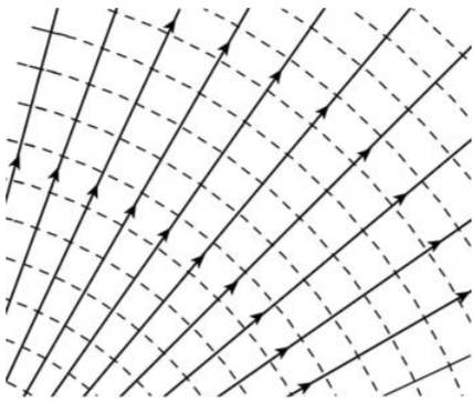
Figure 15.4.1:Surfaces of constant action integral S (dashed lines) and the corresponding particle momenta (solid lines) with arrows showing the direction.

The important role of the action integral $S$ can be illuminated by considering the case of a single point mass $m$ moving in a time independent potential $U(r)$ . Then the action reduces to

S(q, \alpha , t) = W(q, \alpha ) − Et \tag{15.112}

Let $q_1 = x, q_2 = y, q_3 = z, p_1 = p_x, p_2 = p_y, p_3 = p_z$ . The momentum components are given by

p_i = \frac{\partial W(q, \alpha ) }{\partial q_i} \tag{15.113}

which corresponds to

\mathbf{p} = \boldsymbol{\nabla}W = \boldsymbol{\nabla}S \tag{15.114}

That is, the time-independent Hamilton-Jacobi equation is

\frac{1}{2m} |\boldsymbol{\nabla}W|^2 + U(r) = E \tag{15.115}

This implies that the particle momentum is given by the gradient of Hamilton’s characteristic function and is perpendicular to surfaces of constant $W$ as illustrated in Figure 15.4.1. The constant $W$ surfaces are time dependent as given by Equation 15.101. Thus, if at time $t = 0$ the equi-action surface $S_0(q, t) = W_0(q, P_i)=0$ , then at $t = 1$ the same surface $S_0(q, t)=0$ now coincides with the $S_0(q, t) = E$ surface etc. That is, the equi-action surfaces move through space separately from the motion of the single point mass.

The above pictorial representation is analogous to the situation for motion of a wavefront for electromagnetic waves in optics, or matter waves in quantum physics where the wave equation separates into the form $\phi = \phi_0 e^{\frac{ iS}{ \hbar }} = \phi_0 e^{i(\mathbf{k} \cdot \mathbf{r}−\omega t)}$ . Hamilton’s goal was to create a unified theory for optics that was equally applicable to particle motion in classical mechanics. Thus the optical-mechanical analogy of the Hamilton-Jacobi theory has culminated in a universal theory that describes wave-particle duality; this was a Holy Grail of classical mechanics since Newton’s time. It played an important role in development of the Schrödinger representation of quantum mechanics.

Advantages of Hamilton-Jacobi theory¶

Initially, only a few scientists, like Jacobi, recognized the advantages of Hamiltonian mechanics. In 1843 Jacobi made some brilliant mathematical developments in Hamilton-Jacobi theory that greatly enhanced exploitation of Hamiltonian mechanics. Hamilton-Jacobi theory now serves as a foundation for contemporary physics, such as quantum and statistical mechanics. A major advantage of Hamilton-Jacobi theory, compared to other formulations of analytic mechanics, is that it provides a single, first-order partial differential equation for the action $S$ , which is a function of the $n$ generalized coordinates $\mathbf{q}$ and time $t$ . The generalized momenta no longer appear explicitly in the Hamiltonian in equations 15.94, 15.95. Note that the generalized momentum do not explicitly appear in the equivalent Euler-Lagrange equations of Lagrangian mechanics, but these comprise a system of $n$ second-order, partial differential equations for the time evolution of the generalized coordinate $\mathbf{q}$ . Hamilton’s equations of motion are a system of $2n$ first-order equations for the time evolution of the generalized coordinates and their conjugate momenta.

An important advantage of the Hamilton-Jacobi theory is that it provides a formulation of classical mechanics in which motion of a particle can be represented by a wave. In this sense, the Hamilton-Jacobi equation fulfilled a long-held goal of theoretical physics, that dates back to Johann Bernoulli, of finding an analogy between the propagation of light and the motion of a particle. This goal motivated Hamilton to develop Hamiltonian mechanics. A consequence of this wave-particle analogy is that the Hamilton-Jacobi formalism featured prominently in the derivation of the Schrödinger equation during the development of quantum-wave mechanics.

15.5: Action-angle Variables¶

Canonical transformation¶

Systems possessing periodic solutions are a ubiquitous feature in physics. The periodic motion can be either an oscillation, for which the trajectory in phase space is a closed loop (libration), or rolling (rotational) motion as discussed in chapter 3.4. For many problems involving periodic motion, the interest often lies in the frequencies of motion rather than the detailed shape of the trajectories in phase space. The action-angle variable approach uses a canonical transformation to action and angle variables which provide a powerful, and elegant method to exploit Hamiltonian mechanics. In particular, it can determine the frequencies of periodic motion without having to calculate the exact trajectories for the motion. This method was introduced by the French astronomer Ch. E. Delaunay(1816 − 1872) for applications to orbits in celestial mechanics, but it has equally important applications beyond celestial mechanics such as to bound solutions of the atom in quantum mechanics.

The action-angle method replaces the momenta in the Hamilton-Jacobi procedure by the action phase integral for the closed loop (libration) trajectory in phase space defined by

J_i \equiv \oint p_idq_i \tag{15.116}

where for each cyclic variable the integral is taken over one complete period of oscillation. The cyclic variable $I_i$ is called the action variable where

I_i \equiv \frac{1}{ 2\pi} J_i = \frac{1}{ 2\pi} \oint p_idq_i \tag{15.117}

The canonical variable to the action variable $\mathbf{I}$ is the angle variable $\boldsymbol{\phi}$ . Note that the name “action variable” is used to differentiate $\mathbf{I}$ from the action functional $S = \int Ldt$ which has the same units; i.e. angular momentum.

The general principle underlying the use of action-angle variables is illustrated by considering one body, of mass $m$ , subject to a one-dimensional bound conservative potential energy $U(q)$ . The Hamiltonian is given by

H(p,q) = \frac{p^2}{ 2m} + U(q) \tag{15.118}

This bound system has a $(q,p)$ phase space contour for each energy $H = E$ .

p(q,E) = \pm \sqrt{2m(E − U(q))} \tag{15.119}

For an oscillatory system the two-valued momentum of Equation 15.119 is non-trivial to handle. By contrast, the area $J \equiv \oint pdq$ of the closed loop in phase space is a single-valued scalar quantity that depends on $E$ and $U(q)$ . Moreover, Liouville’s theorem states that the area of the closed contour in phase space $J \equiv \oint pdq$ is invariant to canonical transformations. These facts suggest the use of a new pair of conjugate variables, $(\phi , I)$ , where $I(E)$ uniquely labels the trajectory, and corresponding area, of a closed loop in phase space for each value of $E$ , and the single-valued function $\phi$ is a corresponding angle that specifies the exact point along the phase-space contour as illustrated in Fig 15.5.1.

For simplicity consider the linear harmonic oscillator where

U(q) = \frac{1}{ 2} m\omega^2q^2 \tag{15.120}

Then the Hamiltonian, 15.118 equals

H(p,q) = \frac{p^2 }{2m} + \frac{1}{ 2} m\omega^2q^2 \tag{15.121}

Hamilton’s equations of motion give that

\dot{p} = −\frac{\partial H}{ \partial q} = −m\omega^2q \tag{15.122}

\dot{q} = \frac{\partial H}{ \partial p} = \frac{p}{ m} \tag{15.123}

The solution of equations 15.122 and 15.123 is of the form

q = C \cos(\omega (t − t_0)) \tag{15.124}

p = −m\omega C \sin \omega (t − t_0) \tag{15.125}

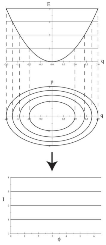
where $C$ , and $t_0$ are integration constants. For the harmonic oscillator, equations 15.124 and 15.125 correspond to the usual elliptical contours in phase space, as illustrated in Figure 15.5.1.

The potential energy V (q), (upper) and corresponding phase space (p,q) (middle) for the harmonic oscillator at four equally spaced total energies E. The corresponding action-angles (I \phi) resulting from a canonical transformation of this system are shown in the lower plot. — Figure 15.5.1:The potential energy $V (q)$ , (upper) and corresponding phase space $(p,q)$ (middle) for the harmonic oscillator at four equally spaced total energies $E$ . The corresponding action-angles $(I \phi)$ resulting from a canonical transformation of this system are shown in the lower plot.

The action-angle canonical transformation involves making the transform

(q,p) \rightarrow (\phi , I) \tag{15.126}

where $I$ is defined by Equation 15.117 and the angle $\phi$ being the corresponding canonical angle. The logical approach to this canonical transformation for the harmonic oscillator is to define $q$ and $p$ in terms of $\phi$ and $I$

q = \sqrt{\frac{ 2I}{ m\omega}} \cos \phi \tag{15.127}

p = \sqrt{2mI\omega } \sin \phi \tag{15.128}

Note that the Poisson bracket is unity

[q, p]_{(\phi , I)} = 1 \nonumber

which implies that the above transformation is canonical, and thus the phase space area $I(E) \equiv \frac{1}{ 2\pi} \oint pdq$ is conserved.

For this canonical transformation the transformed Hamiltonian $\mathcal{H} (\phi , I)$ is

\mathcal{H} (\phi , I) = \frac{1}{ 2m } (2m\omega I) \sin^2 \phi + \frac{1}{ 2 }m\omega^2 \frac{2I}{ m\omega } \cos^2 \phi = \omega I \tag{15.129}

Note that this Hamiltonian is a constant that is independent of the angle $\phi$ , and thus Hamilton’s equations of motion give

\dot{ I} = −\frac{\partial \mathcal{H} (\phi , I)}{ \partial \phi} = 0 \tag{15.130}

\dot{\phi} = \frac{\partial \mathcal{H} (\phi , I) }{\partial I} = \omega \tag{15.131}

Thus we have mapped the harmonic oscillator to new coordinates $(\phi , I)$ where

I = \frac{\mathcal{H} (\phi , I)}{ \omega} = \frac{E }{\omega} \tag{15.132}

\phi = \omega (t − t_0) \tag{15.133}

That is, the phase space has been mapped from ellipses, with area proportional to $E$ in the $(q,p)$ phase space, to a cylindrical $(\phi , I)$ phase space where $I = \frac{E}{\omega}$ are constant values that are independent of the angle, while $\phi$ increases linearly with time. Thus the variables $(q,p)$ are periodic with modulus $\Delta\phi = 2\pi$ .

q(\phi + 2\pi, I) = q (\phi , I) \tag{15.134}

p(\phi + 2\pi, I) = p (\phi , I) \tag{15.135}

The period $\tau$ of the periodic oscillatory motion is given simply by $\Delta\phi = 2\pi = \omega \tau$ which is the well known result for the harmonic oscillator. Note that the action-angle variable canonical transformation has determined the frequency of the periodic motion without solving the detailed trajectory of the motion.

The above example of the harmonic oscillator has shown that, for integrable periodic systems, it is possible to identify a canonical transformation to $(\phi , I)$ such that the Hamiltonian is independent of the angle $\phi$ which specifies the instantaneous location on the constant energy contour $I$ . If the phase space contour is a separatrix, then it divides phase space into invariant regions containing phase-space contours with differing behavior. The action-angle variables are not useful for separatrix contours. For rolling motion, the system rotates with continuously increasing, or decreasing angle, and there is no natural boundary for the action angle variable since the phase space trajectory is continuous and not closed. However, the action-angle approach still is valid if the motion involves periodic as well as rolling motion.

The example of the one-dimensional, one-body, harmonic oscillator can be expanded to the more general case for many bodies in three dimensions. This is illustrated by considering multiple periodic systems for which the Hamiltonian is conservative and where the equations of the canonical transformation are separable. The generalized momenta then can be written as

p_i = \frac{\partial W_i (q_i; \alpha_1, \alpha_2, ..\alpha_n)}{ \partial q_i} \tag{15.136}

for which each $p_i$ is a function of $q_i$ and the $n$ integration constants $\alpha_j$

p_i = p_i (q_i, \alpha_1, \alpha_2, ..\alpha_n) \tag{15.137}

The momentum $p_i (q_i, \alpha_1, \alpha_2, ..\alpha_n)$ represents the trajectory of the system in the $(q_i, p_i)$ phase space that is characterized by Hamilton’s characteristic function $W(q,J)$ . Combining equations 15.116, 15.136 gives

J_i \equiv \oint \frac{\partial W_i (q_i; \alpha_1, \alpha_2, ..\alpha_n)}{ \partial q_i} dq_i \tag{15.138}

Since $q_i$ is merely a variable of integration, each active action variable $J_i$ is a function of the $n$ constants of integration in the Hamilton-Jacobi equation. Because of the independence of the separable-variable pairs $(q_i, p_i)$ , the $J_i$ form $n$ independent functions of the $\alpha_i$ , and hence are suitable for use as a new set of constant momenta. Thus the characteristic function $W$ can be written as

W (q_1, ...q_n; J_1, ...J_n) = \sum_j W_j (q_j ; J_1, ...J_n) \tag{15.139}

while the Hamiltonian is only a function of the momenta $H (J_1, .... J_n)$

The generalized coordinate, conjugate to $J$ , is known as the angle variable $\phi_i$ which is defined by the transformation equation

\phi_i = \frac{\partial W }{\partial J_i} = \sum^n_{j=1} \frac{\partial W_j (q_j ; J_1, ...J_n)}{ \partial J_i} \tag{15.140}

The corresponding equation of motion for $\phi$ is given by

\dot{\phi}_i = \frac{\partial H(J) }{\partial J_i} = 2\pi\omega_i(J_1, ...J_n) \tag{15.141}

where $\omega_i(J)$ are constant functions of the action variables $J_j$ with a solution

\phi_i = 2\pi\omega_it + \beta_i \tag{15.142}

that is, they are linear functions of time. The constants $\omega_i$ can be identified with the frequencies of the multiple periodic motions.

The action-angle variables appear to be no different than a particular set of transformed coordinates. Their merit appears when the physical interpretation is assigned to $\omega_i$ . Consider the change $\delta \phi_i$ as the $q_j$ are changed infinitesimally

\delta \phi_i = \sum_j \frac{\partial \phi_i}{ \partial q_j} \partial q_j = \sum_j \frac{\partial^2 W }{\partial J_i\partial q_j } \partial q_j \tag{15.143}

The derivative with respect to $q_i$ vanishes except for the $W_j$ component of $W$ . Thus Equation 15.143 reduces to

\delta \phi_i = \frac{\partial}{ \partial J_i} \sum_j p_j (q_j , J) dq_j \tag{15.144}

Therefore, the total change in $\phi$ , as the system goes through one complete cycle is

\Delta\phi_i = \sum_j \frac{\partial}{ \partial J_i} \oint p_j (q_j , J) dq_j = 2\pi\delta_{ij} \tag{15.145}

where $\frac{\partial }{ \partial J_i}$ is outside the integral since the $J_i$ are constants for cyclic motion. Thus $\Delta\phi_i = 2\pi = \omega_i\tau_i$ where $\tau_i$ is the period for one cycle of oscillation, where the angular frequency $\omega_i$ is given by

\frac{\omega_i}{ 2\pi} = \nu_i = \frac{1}{ \tau_i} \tag{15.146}

Thus the frequency $\nu$ associated with the periodic motion is the reciprocal of the period $\tau$ . The secret here is that the derivative of $H$ with respect to the action variable $J$ given by Equation 15.141 directly determines the frequency of the periodic motion without the need to solve the complete equations of motion. Note that multiple periodic motion can be represented by a Fourier expansion of the form

q_k = \sum^{\infty}_{j_1=−\infty} \sum^{\infty}_{j_2=−\infty} ... \sum^{\infty}_{j_n=−\infty} a^k_{j_1,..,j_n} e^{2\pi i(j_1\omega_1+ j_2\omega_2+ j_3\omega_3+..+ j_n\omega_n)} \tag{15.147}

Although the action-angle approach to Hamilton-Jacobi theory does not produce complete equations of motion, it does provide the frequency decomposition that often is the physics of interest. The reason that the powerful action-angle variable approach has been introduced here is that it is used extensively in celestial mechanics. The action-angle concept also played a key role in the development of quantum mechanics, in that Sommerfeld recognized that Bohr’s ad hoc assumption that angular momentum is quantized, could be expressed in terms of quantization of the angle variable as is mentioned in chapter 18.

Adiabatic invariance of the action variables¶

When the Hamiltonian depends on time it can be quite difficult to solve for the motion because it is difficult to find constants of motion for time-dependent systems. However, if the time dependence is sufficiently slow, that is, if the motion is adiabatic, then there exist dynamical variables that are almost constant which can be used to solve for the motion. In particular, such approximate constants are the familiar action-angle integrals. The adiabatic invariance of the action variables played an important role in the development of quantum mechanics during the 1911 Solvay Conference. This was a time when physicists were grappling with the concepts of quantum mechanics. Einstein used the following classical mechanics example of adiabatic invariance, applied to the simple pendulum, in order to illustrate the concept of adiabatic invariance of the action. This example demonstrates the power of using action-angle variables.

Example 15.5.1: Adiabatic invariance for the simple pendulum

Consider that the pendulum is made up of a point mass $M$ suspended from a pivot by a light string of length $L$ that is swinging freely in a vertical plane. Derive the dependence of the amplitude of the oscillations $\theta$ , assuming $\theta$ is small, if the string is very slowly shortened by a factor of 2, that is, assume that the change in length during one period of the oscillation is very small. The tension in the string $T$ is given by

T = Mg \langle \cos \theta \rangle + \left\langle \frac{ML^2 \dot{\theta}^2 }{L}\right\rangle \nonumber

Let the pendulum angle be oscillatory

\theta = \theta_0 \cos(\omega t + \varphi_0) \nonumber

Then the average mean square amplitude and velocity over one period are

\langle \theta^2 \rangle = \langle [\theta_0 \cos (\omega t + \varphi_0)]^2 \rangle = \frac{\theta^2_0}{ 2} \nonumber

\left\langle \dot{\theta}^2 \right\rangle = \langle [−\theta_0\omega \sin(\omega t + \varphi_0)]^2\rangle = \frac{\omega^2\theta^2_0}{ 2} \nonumber

Since, for the simple pendulum, $\omega^2 = \frac{g}{L}$ , then the tension in the string

T = Mg(1 − \frac{\langle \theta^2\rangle}{ 2 }) + ML \langle \dot{\theta}^2 \rangle = Mg(1 + \frac{\theta^2_0}{ 4} ) \nonumber

Assuming that $\theta_0$ is a small angle, and that the change in length $−\Delta L$ is very small during one period $\tau$ , then the work done is

\Delta W = T\Delta L = −Mg\Delta L − Mg \frac{\theta^2_0}{4} \Delta L \tag{a}

while the change in internal oscillator energy is

\Delta(−Mg L \cos \theta_0) = \Delta \left[ −Mg L(1 − \frac{\theta^2_0}{2} ) \right] = −Mg\Delta L + \frac{1}{ 2} Mg\Delta( L\theta^2_0) = −Mg\Delta L + \frac{1}{ 2} Mg\theta^2_0\Delta L + Mg L\theta_0 \Delta\theta_0 \tag{b}

The work done must balance the increment in internal energy therefore

L\theta_0\Delta\theta_0 + \frac{3\theta^2_0\Delta L}{ 4} = 0 \nonumber

L\theta^2_0\Delta \ln (\theta_0 L^{\frac{3}{ 4}} )=0 \nonumber

Therefore it follows that

(\theta_0 L^{\frac{3}{ 4}} ) = \text{ constant} \tag{c}

\theta_0 \propto L^{−\frac{ 3}{ 4}} \nonumber

Thus shortening the length of the pendulum string from $L$ to $\frac{L}{2}$ adiabatically corresponds to the amplitude increasing by a factor 1.68.

Consider the action-angle integral for one closed period $\tau = \frac{2\pi}{ \omega}$ for this problem

J = \oint P_{\theta} d\theta \\ = \oint ML^2 \dot{\theta} \cdot \dot{\theta} dt \\ = ML^2 \langle \dot{\theta}^2 \rangle \frac{2\pi}{ \omega} \\ = \pi ML^2\theta^2_0\omega \\= \pi Mg^{\frac{1}{ 2}} \theta^2_0 L^{\frac{3}{ 2}} = \text{ constant} \nonumber

where that last step is due to Equation c.

The above example shows that the action integral $J = constant$ , that is, it is invariant to an adiabatic change. In retrospect this result is as expected in that the action integral should be minimized.

15.6: Canonical Perturbation Theory¶

Most examples in classical mechanics discussed so far have been capable of exact solutions. In real life, the majority of problems cannot be solved exactly. For example, in celestial mechanics the two-body Kepler problem can be solved exactly, but solution of the three-body problem is intractable. Typical systems in celestial mechanics are never as simple as the two-body Kepler system because of the influence of additional bodies. Fortunately in most cases the influence of additional bodies is sufficiently small to allow use of perturbation theory. That is, the restricted three-body approximation can be employed for which the system is reduced to considering it as an exactly solvable two-body problem, subject to a small perturbation to this solvable two-body system. Note that even though the change in the Hamiltonian due to the perturbing term may be small, the impact on the motion can be especially large near a resonance.

Consider the Hamiltonian, subject to a time-dependent perturbation, is written as

H(q, p, t) = H_0(q, p, t) + \Delta H(q, p, t) \nonumber

where $H_0(q, p, t)$ designates the unperturbed Hamiltonian and $\Delta H(q, p, t)$ designates the perturbing term. For the unperturbed system the Hamilton-Jacobi equation is given by

\mathcal{H}(Q_i, P_i, t) = H_0(q_1, ...q_n; \frac{\partial S}{\partial q_1} ..., \frac{\partial S}{\partial q_n };t) + \frac{\partial S}{\partial t} = 0 \tag{15.90}

where $S(q_i, P_i, t)$ is the generating function for the canonical transformation $(q, p) \rightarrow (Q, P)$ . The perturbed $S(q_i, P_i, t)$ remains a canonical transformation, but the transformed Hamiltonian $\mathcal{H}(Q_i, P_i, t) \neq 0$ . That is,

\mathcal{H}(Q_i, P_i, t) = H_0 + \Delta H(q, p, t) + \frac{\partial S}{\partial t} = \Delta H(q, p, t) \tag{15.148}

The equations of motion satisfied by the transformed variables now are

\dot{Q}_i = \frac{\partial \Delta H}{ \partial P_i} \tag{15.149} \\ \dot{P}_i = \frac{\partial \Delta H }{\partial Q_i}

These equations remain as difficult to solve as the full Hamiltonian. However, the perturbation technique assumes that $\Delta H$ is small, and that one can neglect the change of $(Q_i, P_i)$ over the perturbing interval. Therefore, to a first approximation, the unperturbed values of $\frac{\partial \Delta H }{\partial P_i}$ and $\frac{\partial \Delta H}{ \partial Q_i }$ can be used in equations 15.149. A detailed explanation of canonical perturbation theory is presented in chapter 12 of Goldstein[Go50].

Example 15.6.1: Harmonic oscillator perturbation

(a) Consider first the Hamilton-Jacobi equation for the generating function $S(q, \alpha , t)$ for the case of a single free particle subject to the Hamiltonian $H = \frac{1}{ 2} p^2$ . Find the canonical transformation $q = q(\beta ,\alpha )$ and $p = p(\beta ,\alpha )$ where $\beta$ and $\alpha$ are the transformed coordinate and momentum respectively.

The Hamilton-Jacobi equation

\frac{\partial S}{\partial t} + H(q, p, t)=0 \nonumber

Using $p = \frac{\partial S}{\partial q}$ in the Hamiltonian $H = \frac{1}{ 2} p^2$ gives

\frac{\partial S}{\partial t} + \frac{1}{ 2} \left(\frac{\partial S}{\partial q} \right)^2 = 0 \nonumber

Since $H$ does not depend on $q, t$ explicitly, then the two terms on the left hand side of the equation can be set equal to $−\gamma , \gamma$ respectively, where $\gamma$ is at most a function of $p$ . Then the generating function is

S = \sqrt{2\gamma }q − \gamma t \nonumber

Set $\alpha = \sqrt{2\gamma}$ then the generating function can be written as

S = \alpha q − \frac{1}{ 2} \alpha^2t \nonumber

The constant $\alpha$ can be identified with the new momentum $P$ . Then the transformation equations become

p = \frac{\partial S}{\partial q} = \alpha \quad Q = \frac{\partial S}{\partial P} = \frac{\partial S}{\partial \alpha } = q − \alpha t = \beta \nonumber

That is

q = \beta + \alpha t \nonumber

which corresponds to motion with a uniform velocity $\alpha$ in the $q, p$ system.

(b) Consider that the Hamiltonian is perturbed by addition of potential $U = \frac{q^2}{ 2}$ which corresponds to the harmonic oscillator. Then

H = \frac{1}{ 2} p^2 + \frac{q^2}{ 2} \nonumber

Consider the transformed Hamiltonian

\mathcal{H} = H + \frac{\partial S}{\partial t} = \frac{1}{ 2} p^2 + \frac{q^2}{ 2} − \frac{\alpha^2}{ 2} = \frac{q^2}{ 2} = \frac{1}{ 2} (\beta + \alpha t)^2 \nonumber

Hamilton’s equations of motion

\dot{Q} = \frac{\partial \mathcal{H}}{ \partial P} \quad \dot{P} = −\frac{\partial \mathcal{H}}{ \partial Q} \nonumber

give that

\dot{\beta} = (\beta + \alpha t)t \nonumber

\dot{\alpha } = − (\beta + \alpha t) \nonumber

These two equations can be solved to give

\ddot{\alpha} + \alpha = 0 \nonumber

which is the equation of a harmonic oscillator showing that $\alpha$ is harmonic of the form $\alpha = \alpha_0 \sin (t + \delta )$ where $\alpha_0, \delta$ are constants of motion. Thus

\beta = −\dot{\alpha} − t = −\alpha_0 [ \cos(t + \delta ) + t \sin(t + \delta )] \nonumber

The transformation equations then give

p = \alpha = \alpha_0 \sin (t + \delta ) \nonumber

q = \beta + \alpha t = − \dot{\alpha} = −\alpha_0 \cos (t + \delta ) \nonumber

Hence the solution for the perturbed system is harmonic, which is to be expected since the potential has a quadratic dependence of position.

Example 15.6.2: Lindblad resonance in planetary and galactic motion

Use of canonical perturbation theory in celestial mechanics has been exploited by Professor Alice Quillen and her group. They combine use of action-angle variables and Hamilton-Jacobi theory to investigate the role of Lindblad resonance to planetary motion, and also for stellar motion in galaxies. A Lindblad resonance is an orbital resonance in which the orbital period of a celestial body is a simple multiple of some forcing frequency. Even for very weak perturbing forces, such resonance behavior can lead to orbit capture and chaotic motion.

For planetary motion the planet masses are about $1/1000$ that of the central star, so the perturbations to Kepler orbits are small. However, Lindblad resonance for planetary motion led to Saturn’s rings which result from perturbations produced by the moons of Saturn that skulpt and clear dust rings. Stellar orbits in disk galaxies are perturbed a few percent by non axially-symmetric galactic features such as spiral arms or bars. Lindblad resonances perturb stellar motion and drive spiral density waves at distances from the center of a galactic disk where the natural frequency of the radial component of a star’s orbital velocity is close to the frequency of the fluctuations in the gravitational field due to passage through spiral arms or bars. If a stars orbital speed around a galactic center is greater than that of the part of a spiral arm through which it is traversing, then an inner Lindblad resonance occurs which speeds up the star’s orbital speed moving the orbit outwards. If the orbital speed is less than that of a spiral arm, an inner Lindblad resonance occurs causing inward movement of the orbit.

15.7: Symplectic Representation¶

The Hamilton’s first-order equations of motion are symmetric if the generalized and constraint force terms, in equation $(15.1.9)$ , are excluded.

\mathbf{\dot{q}} = \frac{\partial H}{ \partial \mathbf{p}} \quad − \mathbf{\dot{p}} = \frac{\partial H}{ \partial \mathbf{q}} \nonumber

This stimulated attempts to treat the canonical variables $(\mathbf{q}, \mathbf{p})$ in a symmetric form using group theory. Some graduate textbooks in classical mechanics have adopted use of symplectic symmetry in order to unify the presentation of Hamiltonian mechanics. For a system of $n$ degrees of freedom, a column matrix $\boldsymbol{\eta}$ is constructed that has $2n$ elements where

\eta_j = q_j \quad \eta_{n+j} = p_j \quad j \leq n \tag{15.150}

Therefore the column matrix

\left(\frac{\partial H}{ \partial \boldsymbol{\eta}} \right)_j = \frac{\partial H }{\partial q_j} \quad \left(\frac{\partial H}{ \partial \boldsymbol{\eta}} \right)_{n+j} = \frac{\partial H }{\partial p_j} \quad j \leq n \tag{15.151}

The symplectic matrix $\mathbf{J}$ is defined as being a $2n$ by $2n$ skew-symmetric, orthogonal matrix that is broken into four $n \times n$ null or unit matrices according to the scheme

\mathbf{J} = \begin{pmatrix} [\mathbf{0}] & +[\mathbf{1}] \\ − [\mathbf{1}] & [\mathbf{0}] \end{pmatrix} \tag{15.152}

where $[\mathbf{0}]$ is the $n$ -dimension null matrix, for which all elements are zero. Also $[\mathbf{1}]$ is the $n$ -dimensional unit matrix, for which the diagonal matrix elements are unity and all off-diagonal matrix elements are zero. The $\mathbf{J}$ matrix accounts for the opposite signs used in the equations for $\mathbf{\dot{q}}$ and $\mathbf{\dot{p}}$ . The symplectic representation allows the Hamilton’s equations of motion to be written in the compact form

\boldsymbol{\dot{\eta}} = \mathbf{J}\frac{\partial H }{\partial \boldsymbol{\eta}} \tag{15.153}

This textbook does not use the elegant symplectic representation since this representation ignores the important generalized forces and Lagrange multiplier forces.

15.8: Comparison of the Lagrangian and Hamiltonian Formulations¶

Common features¶

The discussion of Lagrangian and Hamiltonian dynamics has illustrated the power of such algebraic formulations. Both approaches are based on application of variational principles to scalar energy which gives the freedom to concentrate solely on active forces and to ignore internal forces. Both methods can handle manybody systems and exploit canonical transformations, which are impractical or impossible using the vectorial Newtonian mechanics. These algebraic approaches simplify the calculation of the motion for constrained systems by representing the vector force fields, as well as the corresponding equations of motion, in terms of either the Lagrangian function $L(\mathbf{q}, \mathbf{\dot{q}}, t)$ or the action functional $S(\mathbf{q},\mathbf{p},t)$ which are related by the definite integral

S(\mathbf{q},\mathbf{p},t) = \int^{t_2}_{t_1} L(\mathbf{q}, \mathbf{\dot{q}}, t)dt \tag{15.1}

The Lagrangian function $L(\mathbf{q}, \mathbf{\dot{q}}, t)$ , and the action functional $S(\mathbf{q},\mathbf{p},t)$ , are scalar functions under rotation, but they determine the vector force fields and the corresponding equations of motion. Thus the use of rotationally-invariant functions $L(\mathbf{q}, \mathbf{\dot{q}}, t)$ and $S(\mathbf{q},\mathbf{p},t)$ provide a simple representation of the vector force fields. This is analogous to the use of scalar potential fields $\phi (\mathbf{q}, t)$ to represent the electrostatic and gravitational vector force fields. Like scalar potential fields, Lagrangian and Hamiltonian mechanics represents the observables as derivatives of $L(\mathbf{q}, \mathbf{\dot{q}}, t)$ and $S(\mathbf{q},\mathbf{p},t)$ , and the absolute values of $L(\mathbf{q}, \mathbf{\dot{q}}, t)$ and $S(\mathbf{q},\mathbf{p},t)$ are undefined; only differences in $L(\mathbf{q}, \mathbf{\dot{q}}, t)$ and $S(\mathbf{q},\mathbf{p},t)$ are observable. For example, the generalized momenta are given by the derivatives $p_i \equiv \frac{\partial L}{ \partial \dot{q}_i}$ and $p_j = \frac{\partial S }{\partial q_j }$ . The physical significance of the least action $S(\mathbf{q}, \boldsymbol{\alpha},t)$ is illustrated when the canonically transformed momenta $\mathbf{P} = \boldsymbol{\alpha}$ is a constant. Then the generalized momenta and the Hamilton-Jacobi equation, imply that the total time derivative of the action equals

\frac{dS}{ dt} = \frac{\partial S}{ \partial q_i} \dot{q}_i + \frac{\partial S}{ \partial t} = p_iq_i − H = L \tag{15.154}

The indefinite integral of this equation reproduces the definite integral 15.1 to within an arbitrary constant, i.e.

S(\mathbf{q}, \mathbf{p}) = \int L(\mathbf{q}, \mathbf{\dot{q}}, t)dt + \text{ constant} \tag{15.155}

Lagrangian Formulation¶

Consider a system with $n$ independent generalized coordinates, plus $m$ constraint forces that are not required to be known. The Lagrangian approach can reduce the system to a minimal system of $s = n − m$ independent generalized coordinates leading to $s = n - m$ second-order differential equations. By comparison, the Newtonian approach uses $n + m$ unknowns. Alternatively, the Lagrange multipliers approach allows determination of the holonomic constraint forces resulting in $s = n + m$ second order equations to determine $s = n + m$ unknowns. The Lagrangian potential function is limited to conservative forces, but generalized forces can be used to handle non-conservative and non-holonomic forces. The advantage of the Lagrange equations of motion is that they can deal with any type of force, conservative or non-conservative, and they directly determine $q, \dot{q}$ rather than $q,p$ which then requires relating $p$ to $\dot{q}$ . The Lagrange approach is superior to the Hamiltonian approach if a numerical solution is required for typical undergraduate problems in classical mechanics. However, Hamiltonian mechanics has a clear advantage for addressing more profound and philosophical questions in physics.

Hamiltonian Formulation¶

For a system with $n$ independent generalized coordinates, and $m$ constraint forces, the Hamiltonian approach determines $2n$ first-order differential equations. In contrast to Lagrangian mechanics, where the Lagrangian is a function of the coordinates and their velocities, the Hamiltonian uses the variables $\mathbf{q}$ and $\mathbf{p}$ , rather than velocity. The Hamiltonian has twice as many independent variables as the Lagrangian which is a great advantage, not a disadvantage, since it broadens the realm of possible transformations that can be used to simplify the solutions. Hamiltonian mechanics uses the conjugate coordinates $\mathbf{q},\mathbf{p}$ , corresponding to phase space. This is an advantage in most branches of physics and engineering. Compared to Lagrangian mechanics, Hamiltonian mechanics has a significantly broader arsenal of powerful techniques that can be exploited to obtain an analytical solution of the integrals of the motion for complicated systems. These techniques include, the Poisson bracket formulation, canonical transformations, the Hamilton-Jacobi approach, the action-angle variables, and canonical perturbation theory. In addition, Hamiltonian dynamics provides a means of determining the unknown variables for which the solution assumes a soluble form, and it is ideal for study of the fundamental underlying physics in applications to other fields such as quantum or statistical physics. However, the Hamiltonian approach endemically assumes that the system is conservative putting it at a disadvantage with respect to the Lagrangian approach. The appealing symmetry of the Hamiltonian equations, plus their ability to utilize canonical transformations, makes it the formalism of choice for examination of system dynamics. For example, Hamilton-Jacobi theory, action-angle variables and canonical perturbation theory are used extensively to solve complicated multibody orbit perturbations in celestial mechanics by finding a canonical transformation that transforms the perturbed Hamiltonian to a solved unperturbed Hamiltonian.

The Hamiltonian formalism features prominently in quantum mechanics since there are well established rules for transforming the classical coordinates and momenta into linear operators used in quantum mechanics. The variables $\mathbf{q}, \mathbf{\dot{q}}$ used in Lagrangian mechanics do not have simple analogs in quantum physics. As a consequence, the Poisson bracket formulation, and action-angle variables of Hamiltonian mechanics played a key role in development of matrix mechanics by Heisenberg, Born, and Dirac, while the Hamilton-Jacobi formulation played a key role in development of Schrödinger’s wave mechanics. Similarly, Hamiltonian mechanics is the preeminent variational approached used in statistical mechanics.

15.E: Advanced Hamiltonian Mechanics (Exercises)¶

Poisson brackets are a powerful means of elucidating when observables are constant of motion and whether two observables can be simultaneously measured with unlimited precision. Consider a spherically symmetric Hamiltonian
$H = \frac{1}{2m} \left( p^2_r + \frac{p^{2}_{\theta}}{r^2} + \frac{p^2_{\phi}}{r^2 \sin^2 \theta} \right) + U(r) \nonumber$
for a mass $m$ where $U(r$ is a central potential. Use the Poisson bracket plus the time dependence to determine the following:
Does $p_{\phi}$ commute with $H$ and is it a constant of motion?
Does $p^2_{\theta} + \frac{p^2_{\phi}}{ \sin^2 \theta }$ commute with $H$ and is it a constant of motion?
Does $p_r$ commute with $H$ and is it a constant of motion?
Does $p_{\phi}$ commute with $p_{\theta}$ and what does the result imply?
Consider the Poisson brackets for angular momentum $L$
Show $\{L_i, r_j \} = \epsilon_{ijk}r_k$ , where the Levi-Cevita tensor is,
$\epsilon_{ijk} = \begin{cases} +1 & \mbox{if } ijk \mbox{ are cyclically permuted}\\ −1 & \mbox{if } ijk \mbox{ are anti-cyclically permuted} \\ 0 & \mbox{if } i = j \mbox{ or } i = k \mbox{ or } j = k \end{cases} \nonumber$
Show $\{L_i, p_j \} = \epsilon_{ijk}p_{k}$ .
Show $\{L_i, L_j \} = \epsilon_{ijk}L_k$ . The following identity may be useful: $\epsilon_{ijk}\epsilon_{ilm} = \delta_{jl}\delta_{km} − \delta_{jm}\delta_{kl }$ .
Show $\{L_i, L^2 \} = 0$ .
Consider the Hamiltonian of a two-dimensional harmonic oscillator,
$H = \frac{\mathbf{p}^2 }{2m} + \frac{1 }{2 }m ( \omega^2_1r^2_1 + \omega^2_2r^2_2 ) \nonumber$
What condition is satisfied if $L^2$ a conserved quantity?
Consider the motion of a particle of mass $m$ in an isotropic harmonic oscillator potential $U = \frac{1}{ 2} kr^2$ and take the orbital plane to be the $x − y$ plane. The Hamiltonian is then
$H \equiv S_0 = \frac{1}{2m}(p^2_x + p^2_y) +\frac{1}{2}k(x^2 + y^2) \nonumber$

Introduce the three quantities

S_1 = \frac{1}{2m}(p^2_x − p^2_y) +\frac{1}{2}k(x^2 − y^2) \nonumber

S_2 = \frac{1}{ m} p_{x}p_{y} + kxy \nonumber

S_3 = \omega (xp_{y} − yp_{x}) \nonumber

with $\omega = \sqrt{\frac{k}{m}}$ . Use Poisson brackets to solve the following:

Show that $\{S_0, S_i\}=0$ for $i = 1, 2, 3$ proving that $(S_1, S_2, S_3)$ are constants of motion.
Show that
$\{S_1, S_2\}=2\omega S_3 \nonumber$

\{S_2, S_3\}=2\omega S_1 \nonumber

\{S_3, S_1\}=2\omega S_2 \nonumber

so that $(2\omega )^{ −1 } (S_1, S_2, S_3)$ have the same Poisson bracket relations as the components of a 3-dimensional angular momentum.

S^2_0 = S^2_1 + S^2_2 + S^2_3 \nonumber

Assume that the transformation equations between the two sets of coordinates $(q, p)$ and $(Q, P)$ are

Q = \ln (1 + q^{\frac{1}{2}} \cos p) \nonumber

P = 2(1 + q^{\frac{1}{2}} \cos p)q^{\frac{1}{2}} \sin p) \nonumber

Assuming that $q, p$ are canonical variables, i.e. $[q, p]=1$ , show directly from the above transformation equations that $Q, P$ are canonical variables.
Show that the generating function that generates this transformation between the two sets of canonical variables is
$F_3 = −[e^Q − 1]^2 \tan p \nonumber$
Consider a bound two-body system comprising a mass $m$ in an orbit at a distance $r$ from a mass $M$ . The attractive central force binding the two-body system is

\mathbf{F} = \frac{k}{r^2}\mathbf{\hat{r}} \nonumber

where $k$ is negative. Use Poisson brackets to prove that the eccentricity vector $A = p\times L+\mu k\hat{r}$ is a conserved quantity.

Consider the case of a single mass m where the Hamiltonian $H =\frac{1}{2}p^2$ .
Use the generating function $S(q, P, t)$ to solve the Hamilton-Jacobi equation with the canonical transformation $q = q(Q, P)$ and $p = p(Q, P)$ and determine the equations relating the $(q, p)$ variables to the transformed coordinate and momentum $(Q, P)$ .
If there is a perturbing Hamiltonian $\Delta H =\frac{1}{2}q^2$ , then $P$ will not be constant. Express the transformed Hamiltonian $H$ (using the transformation given above in terms of $P$ , $Q$ , and $t$ ). Solve for $Q(t)$ and $P(t)$ and show that the perturbed solution $q[Q(t), P(t)]$ , $p[Q(t), P(t)]$ is simple harmonic.

15.S: Advanced Hamiltonian mechanics (Summary)¶

This chapter has gone beyond what is normally covered in an undergraduate course in classical mechanics, in order to illustrate the power of the remarkable arsenal of methods available for solution of the equations of motion using Hamiltonian mechanics. This has included the Poisson bracket representation of Hamiltonian formulation of mechanics, canonical transformations, Hamilton-Jacobi theory, action-angle variables, and canonical perturbation theory. The purpose was to illustrate the power of variational principles in Hamiltonian mechanics and how they relate to fields such as quantum mechanics and astronomy. The following are the key points made in this chapter.

Poisson brackets:¶

The elegant and powerful Poisson bracket formalism of Hamiltonian mechanics was introduced. The Poisson bracket of any two continuous functions of generalized coordinates $F(p,q)$ and $G(p,q)$ , is defined to be

\{F, G\}_{pq} \equiv \sum_i \left( \frac{\partial F}{\partial q_i} \frac{\partial G}{\partial p_i} − \frac{\partial F}{\partial p_i} \frac{\partial G}{\partial q_i}\right)

The fundamental Poisson brackets equal

\{q_k, q_l\}=0

\{p_k, p_l\}=0

\{q_k, p_l\} = − \{p_l, q_k\} = \delta_{kl}

The Poisson bracket is invariant to a canonical transformation from $(q, p)$ to $(Q, P)$ . That is

\{F, G\}_{qp} = \sum_k \left( \frac{\partial F}{\partial Q_k} \frac{\partial G}{\partial P_k } − \frac{\partial F}{\partial P_k }\frac{\partial G}{\partial Q_k} \right) = \{F, G\}_{QP}

There is a one-to-one correspondence between the commutator and Poisson Bracket of two independent functions,

(F_1G_1 − G_1F_1) = \lambda \{F_1, G_1\}

where $\lambda$ is an independent constant. In particular $F_1G_1$ commute of the Poisson Bracket $\{F_1, G_1\}=0$ .

Poisson Bracket representation of Hamiltonian mechanics:¶

It has been shown that the Poisson bracket formalism contains the Hamiltonian equations of motion and is invariant to canonical transformations. Also this formalism extends Hamilton’s canonical equations to non-commuting canonical variables. Hamilton’s equations of motion can be expressed directly in terms of the Poisson brackets

\dot{q}_k = \{q_k, H\} = \frac{\partial H }{\partial p_k}

\dot{p}_k = \{p_k, H\} = −\frac{\partial H}{ \partial q_k }

An important result is that the total time derivative of any operator is given by

\frac{dG}{dt} = \frac{\partial G}{\partial t} + \{G, H\}

Poisson brackets provide a powerful means of determining which observables are time independent and whether different observables can be measured simultaneously with unlimited precision. It was shown that the Poisson bracket is invariant to canonical transformations, which is a valuable feature for Hamiltonian mechanics. Poisson brackets were used to prove Liouville’s theorem which plays an important role in the use of Hamiltonian phase space in statistical mechanics. The Poisson bracket is equally applicable to continuous solutions in classical mechanics as well as discrete solutions in quantized systems.

Canonical transformations:¶

A transformation between a canonical set of variables $(q,p)$ with Hamiltonian $H(q,p, t)$ to another set of canonical variable $(Q,P)$ with Hamiltonian $\mathcal{H}(Q,P, t)$ can be achieved using a generating functions $F$ such that

\mathcal{H}(Q,P, t) = H(q,p, t) + \frac{\partial F}{\partial t}

Possible generating functions are summarized in the following table.

Generating function	Generating function derivatives	Trivial special case
$F = F_1 (\mathbf{q}, \mathbf{Q}, t)$	$p_i = \frac{\partial F_1}{\partial q_i} \quad P_i = -\frac{\partial F_1}{\partial Q_i}$	$F_1 = q_iQ_i \quad Q_i = p_i \quad P_i = -q_i$
$F = F_2 (\mathbf{q}, \mathbf{P}, t) - \mathbf{Q} \cdot \mathbf{P}$	$p_i = \frac{\partial F_2}{\partial q_i} \quad Q_i = \frac{\partial F_2}{\partial P_i}$	$F_2 = q_iP_i \quad Q_i = q_i \quad P_i = p_i$
$F = F_3 (\mathbf{p}, \mathbf{Q}, t) + \mathbf{q} \cdot \mathbf{p}$	$q_i = -\frac{\partial F_3}{\partial p_i} \quad P_i = -\frac{\partial F_3}{\partial Q_i}$	$F_3 = p_iQ_i \quad Q_i = -q_i \quad P_i = -p_i$
$F = F_4 (\mathbf{p}, \mathbf{P}, t) + \mathbf{q} \cdot \mathbf{p} - \mathbf{Q} \cdot \mathbf{P}$	$q_i = -\frac{\partial F_4}{\partial p_i} \quad Q_i = \frac{\partial F_4}{\partial P_i}$	$F_1 = p_iP_i \quad Q_i = p_i \quad P_i = -q_i$

If the canonical transformation makes $\mathcal{H}(Q,P, t)=0$ then the conjugate variables $(Q,P)$ are constants of motion. Similarly if $\mathcal{H}(Q,P, t)$ is a cyclic function then the corresponding $P$ are constants of motion.

Hamilton-Jacobi theory:¶

Hamilton-Jacobi theory determines the generating function required to perform canonical transformations that leads to a powerful method for obtaining the equations of motion for a system. The Hamilton-Jacobi theory uses the action function $S \equiv F_2$ as a generating function, and the canonical momentum is given by

p_i = \frac{\partial S}{ \partial q_i}

This can be used to replace $p_i$ in the Hamiltonian $H$ leading to the Hamilton-Jacobi equation

H(q; \frac{\partial S}{ \partial q} ;t) + \frac{\partial S}{ \partial t} = 0

Solutions of the Hamilton-Jacobi equation were obtained by separation of variables. The close optical-mechanical analogy of the Hamilton-Jacobi theory is an important advantage of this formalism that led to it playing a pivotal role in the development of wave mechanics by Schrödinger.

Action-angle variables:¶

The action-angle variables exploits a canonical transformation from $(q,p) \rightarrow (\phi , I)$ where

I_i \equiv \frac{1}{ 2\pi} J_i = \frac{1}{ 2\pi} \oint p_i dq_i

For periodic motion the phase-space trajectory is closed with area given by $J$ and this area is conserved for the above canonical transformation. For a conserved Hamiltonian the action variable $I$ is independent of the angle variable $\phi$ . The time dependence of the angle variable $\phi$ directly determines the frequency of the periodic motion without recourse to calculation of the detailed trajectory of the periodic motion.

Canonical perturbation theory:¶

Canonical perturbation theory is a valuable method of handling multibody interactions. The adiabatic invariance of the action-angle variables provides a powerful approach for exploiting canonical perturbation theory.

Comparison of Lagrangian and Hamiltonian formulations:¶

The remarkable power, and intellectual beauty, provided by use of variational principles to exploit the underlying principles of natural economy in nature, has had a long and rich history. It has led to profound developments in many branches of theoretical physics. However, it is noted that although the above algebraic formulations of classical mechanics have been used for over two centuries, the important limitations of these algebraic formulations to non-linear systems remain a challenge that still is being addressed.

It has been shown that the Lagrangian and Hamiltonian formulations represent the vector force fields, and the corresponding equations of motion, in terms of the Lagrangian function $L(\mathbf{q}, \mathbf{\dot{q}},t)$ , or the action functional $S(\mathbf{q},\mathbf{p},t)$ , which are scalars under rotation. The Lagrangian function $L(\mathbf{q}, \mathbf{\dot{q}},t)$ is related to the action functional $S(\mathbf{q},\mathbf{p},t)$ by

S(\mathbf{q},\mathbf{p},t) = \int^{t_2}_{t_1}L(\mathbf{q}, \mathbf{\dot{q}},t) dt\tag{15.1}

These functions are analogous to electric potential, in that the observables are derived by taking derivatives of the Lagrangian function $L(\mathbf{q}, \mathbf{\dot{q}},t)$ or the action functional $S(\mathbf{q},\mathbf{p},t)$ . The Lagrangian formulation is more convenient for deriving the equations of motion for simple mechanical systems. The Hamiltonian formulation has a greater arsenal of techniques for solving complicated problems plus it uses the canonical variables $(q_i, p_i)$ which are the variables of choice for applications to quantum mechanics and statistical mechanics.

15.1: Introduction to Advanced Hamiltonian Mechanics¶

Action functional SSS:¶

Generalized momentum ppp:¶

Generalized energy h(q,q˙,t)h(\mathbf{q}, \dot{q},t )h(q,q˙​,t):¶

Hamiltonian function:¶

Generalized energy theorem:¶

Hamilton’s equations of motion:¶

Hamilton-Jacobi equation:¶

15.2: Poisson bracket Representation of Hamiltonian Mechanics¶

Poisson Brackets¶

Fundamental Poisson Brackets¶

Poisson bracket invariance to canonical transformations¶

Correspondence of the Commutator and the Poisson Bracket¶

Observables in Hamiltonian mechanics¶

Time dependence:¶

Independence¶

Hamilton’s equations of motion¶

Liouville’s Theorem¶

15.3: Canonical Transformations in Hamiltonian Mechanics¶

Generating functions¶

Type 1: F=F1(q,Q,t)F = F_1(\mathbf{q}, \mathbf{Q},t)F=F1​(q,Q,t):¶

Type 2: F=F2(q,P,t)−Q⋅PF = F_2(\mathbf{q},\mathbf{P},t) − \mathbf{Q} \cdot \mathbf{P}F=F2​(q,P,t)−Q⋅P:¶

Type 3: F=F3(p,Q,t)+q⋅pF = F_3(\mathbf{p}, \mathbf{Q},t) + \mathbf{q} \cdot \mathbf{p}F=F3​(p,Q,t)+q⋅p:¶

Type 4: F=F4(p,P,t)+q⋅p−Q⋅PF = F_4(\mathbf{p}, \mathbf{P},t) + \mathbf{q} \cdot \mathbf{p} − \mathbf{Q} \cdot \mathbf{P}F=F4​(p,P,t)+q⋅p−Q⋅P:¶

Applications of Canonical Transformations¶

15.4: Hamilton-Jacobi Theory¶

Time-dependent Hamiltonian¶

Jacobi’s complete integral S(qi,Pi,t)S(q_i, P_i, t)S(qi​,Pi​,t)¶

Hamilton’s principle function SH(qi,t;qoto)S_H(\mathbf{q}_i, t; \mathbf{q}_o t_o)SH​(qi​,t;qo​to​)¶

Time-independent Hamiltonian¶

Separation of variables¶

Visual representation of the action function SSS.¶

Advantages of Hamilton-Jacobi theory¶

15.5: Action-angle Variables¶

Canonical transformation¶

Adiabatic invariance of the action variables¶

15.6: Canonical Perturbation Theory¶

15.7: Symplectic Representation¶

15.8: Comparison of the Lagrangian and Hamiltonian Formulations¶

Common features¶

Lagrangian Formulation¶

Hamiltonian Formulation¶

15.E: Advanced Hamiltonian Mechanics (Exercises)¶

15.S: Advanced Hamiltonian mechanics (Summary)¶

Poisson brackets:¶

Poisson Bracket representation of Hamiltonian mechanics:¶

Canonical transformations:¶

Hamilton-Jacobi theory:¶

Action-angle variables:¶

Canonical perturbation theory:¶

Comparison of Lagrangian and Hamiltonian formulations:¶

Action functional $S$ :¶

Generalized momentum $p$ :¶

Generalized energy $h(\mathbf{q}, \dot{q},t )$ :¶

Type 1: $F = F_1(\mathbf{q}, \mathbf{Q},t)$ :¶

Type 2: $F = F_2(\mathbf{q},\mathbf{P},t) − \mathbf{Q} \cdot \mathbf{P}$ :¶

Type 3: $F = F_3(\mathbf{p}, \mathbf{Q},t) + \mathbf{q} \cdot \mathbf{p}$ :¶

Type 4: $F = F_4(\mathbf{p}, \mathbf{P},t) + \mathbf{q} \cdot \mathbf{p} − \mathbf{Q} \cdot \mathbf{P}$ :¶

Jacobi’s complete integral $S(q_i, P_i, t)$ ¶

Hamilton’s principle function $S_H(\mathbf{q}_i, t; \mathbf{q}_o t_o)$ ¶

Visual representation of the action function $S$ .¶