9. Hamilton's Action Principle

9. Hamilton’s Action Principle¶

9.1: Introduction to Hamilton’s Action Principle¶

Hamilton’s principle of stationary action was introduced in two papers published by Hamilton in 1834 and 1835. Hamilton’s Action Principle provides the foundation for building Lagrangian mechanics that had been pioneered 46 years earlier. Hamilton’s Principle now underlies theoretical physics and many other disciplines in mathematics and economics. In 1834 Hamilton was seeking a theory of optics when he developed both his principle of stationary action, plus the field of Hamiltonian mechanics.

Hamilton’s Action Principle is based on defining the action functional^[1] $S$ for $n$ generalized coordinates which are expressed by the vector $\mathbf{q,}$ and their corresponding velocity vector $\mathbf{ \dot{q}}$ .

S=\int_{t_{i}}^{t_{f}}L(\mathbf{q,\dot{q},}t\mathbf{)}dt

The scalar action $S,$ is a functional of the Lagrangian $L(\mathbf{q,\dot{q} ,}t\mathbf{)}$ , integrated between an initial time $t_{i}$ and final time $t_{f}$ . In principle, higher order time derivatives of the generalized coordinates could be included, but most systems in classical mechanics are described adequately by including only the generalized coordinates, plus their velocities. The definition of the action functional allows for more general Lagrangians than the standard Lagrangian $L(\mathbf{q,\dot{q},}t)=T( \mathbf{\dot{q},}t)-U(\mathbf{q},t)$ that has been used throughout chapters $5-8$ . Hamilton stated that the actual trajectory of a mechanical system is that given by requiring that the action functional is stationary with respect to change of the variables. The action functional is stationary when the variational principle can be written in terms of a virtual infinitessimal displacement, $\delta ,$ to be

\delta S=\delta \int_{t_{i}}^{t_{f}}L(\mathbf{q,\dot{q},}t\mathbf{)}dt=0

Typically the stationary point corresponds to a minimum of the action functional. Applying variational calculus to the action functional leads to the same Lagrange equations of motion for systems as the equations derived using d’Alembert’s Principle, if the additional generalized force terms, $\sum_{k=1}^{m}\lambda _{k}\frac{\partial g_{k}}{\partial q_{j}}(\mathbf{q} ,t)+Q_{j}^{EXC}$ , are omitted in the corresponding equations of motion.

These are used to derive the equations of motion, which then are solved for an assumed set of initial conditions. Prior to Hamilton’s Action Principle, Lagrange developed Lagrangian mechanics based on d’Alembert’s Principle in contrast to Newtonian equations of motion which are defined in terms of Newton’s Laws of Motion.

9.2: Hamilton’s Principle of Stationary Action¶

Hamilton’s crowning achievement was his use of the general form of Hamilton’s principle of stationary action $S$ , equation $(9.1.2)$ , to derive both Lagrangian mechanics, and Hamiltonian mechanics. Consider the action $S_{A}$ for the extremum path of a system in configuration space, that is, along path $A$ for $j=1,2,\dots ,n$ coordinates $q_{j}(t_{i})$ at initial time $t_{i}$ to $q_{j}(t_{f})$ at a final time $t_{f}$ as shown in Figure 9.2.1.

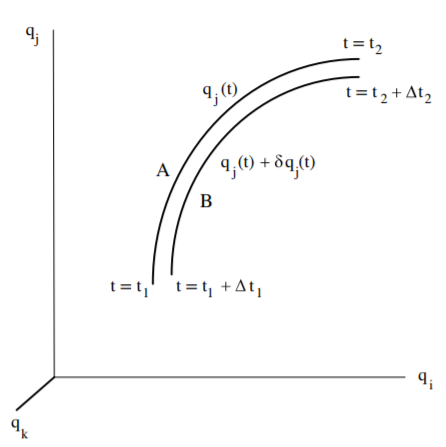
Figure 9.2.1:Extremum path A, plus the neighboring path B, shown in configuration space.

Then the action $S_{A}$ is given by

S_{A}=\int_{t_{i}}^{t_{f}}L(\mathbf{q}(t)\mathbf{, \dot{q}}(t)\mathbf{,}t)dt \tag{9.3}

As used in chapter $5.2,$ a family of neighboring paths is defined by adding an infinitessimal fraction $\epsilon$ of a continuous, well-behaved neighboring function $\eta _{j}$ where $\epsilon =0$ for the extremum path. That is,

q_{j}(t,\epsilon )=q_{j}(t,0)+\epsilon \eta _{j}(t)\tag{9.4}

In contrast to the variational case discussed when deriving Lagrangian mechanics, the variational path used here does not assume that the functions $\eta _{i}(t)$ vanish at the end points. Assume that the neighboring path $B$ has an action $S_{B}$ where

S_{B}=\int_{t_{i}+\Delta t}^{t_{f}+\Delta t}L(\mathbf{q}(t)\mathbf{+\delta q} (t)\mathbf{,\dot{q}}(t)\mathbf{+\delta \dot{q}}(t))dt\tag{9.5}

Expanding the integrand of $S_{B}$ in Equation 9.5 gives that, relative to the extremum path $A$ , the incremental change in action is

\delta S=S_{B}-S_{A}=\int_{t_{i}}^{t_{f}}\sum_{j}\left( \frac{\partial L}{ \partial q_{j}}\delta q_{j}+\frac{\partial L}{\partial \dot{q}_{j}}\delta \dot{q}_{j}\right) dt+\left[ L\Delta t\right] _{t_{i}}^{t_{f}}\tag{9.6}

The second term in the integral can be integrated by parts since $\delta \dot{q}_{j}=d\left( \frac{\delta q_{j}}{dt}\right)$ leading to

\delta S=\int_{t_{i}}^{t_{f}}\sum_{j}\left( \frac{\partial L}{\partial q_{j}} -\frac{d}{dt}\frac{\partial L}{\partial \dot{q}_{j}}\right) \delta q_{j}dt+ \left[ \sum_{j}\frac{\partial L}{\partial \dot{q}_{j}}\delta q_{j}+L\Delta t \right] _{t_{i}}^{t_{f}}\tag{9.7}

Note that Equation 9.7 includes contributions from the entire path of the integral as well as the variations at the ends of the curve and the $\Delta t$ terms. Equation 9.7 leads to the following two pioneering principles of least action in variational mechanics that were developed by Hamilton.

Stationary-action principle in Lagrangian mechanics¶

Derivation of Lagrangian mechanics in chapter 6 was based on the extremum path for neighboring paths between two given locations $\mathbf{q(} t_{i})$ and $\mathbf{q}(t_{f})$ that the system occupies at the initial and final times $t_{i}$ and $t_{f}$ respectively. For this special case, where the end points do not vary, that is, when $\delta q_{i}(t_{i})=\delta q_{i}(t_{f})=0$ , and $\Delta t_{i}=\Delta t_{f}=0$ , then the least action $\delta S$ for the stationary path 9.8 reduces to

\delta S=\int_{t_{i}}^{t_{f}}\sum_{j}\left( \frac{\partial L}{\partial q_{j}} -\frac{d}{dt}\frac{\partial L}{\partial \dot{q}_{j}}\right) \delta q_{j}dt=0\tag{9.8}

For independent generalized coordinates $\delta q_{j}$ , the integrand in brackets vanishes leading to the Euler-Lagrange equations. Conversely, if the Euler-Lagrange equations in 9.8 are satisfied, then, $\delta S=0,$ that is, the path is stationary. This leads to the statement that the path in configuration space between two configurations $\mathbf{q(} t_{i})$ and $\mathbf{q}(t_{f})$ that the system occupies at times $t_{i}$ and $t_{f}$ respectively, is that for which the action $S$ is stationary. This is a statement of Hamilton’s Principle.

Stationary-action principle in Hamiltonian mechanics¶

Hamilton used the general variation of the least-action path to derive the basic equations of Hamiltonian mechanics. For the general path, the integral term in Equation 9.7 vanishes because the Euler-Lagrange equations are obeyed for the stationary path. Thus the only remaining non-zero contributions are due to the end point terms, which can be written by defining the total variation of each end point to be

\Delta q_{j}=\delta q_{j}+\dot{q}_{j}\Delta t\tag{9.9}

where $\delta q_{i}$ and $\dot{q}_{i}$ are evaluated at $t_{i}$ and $t_{f}$ . Then Equation 9.7 reduces to

\delta S=\left[ \sum_{j}\frac{\partial L}{\partial \dot{q}_{j}}\delta q_{j}+L\Delta t\right] _{t_{i}}^{t_{f}}=\left[ \sum_{j}\frac{\partial L}{ \partial \dot{q}_{j}}\Delta q_{j}+\left( -\sum_{j}\frac{\partial L}{\partial \dot{q}_{j}}\dot{q}_{j}+L\right) \Delta t\right] _{t_{i}}^{t_{f}}\tag{9.10}

Since the generalized momentum $p_{j}=\frac{\partial L}{\partial \dot{q}_{j}}$ , then Equation 9.10 can be expressed in terms of the Hamiltonian and generalized momentum as

\tag{9.11} \delta S = \left[ \sum_{j}p_{j}\Delta q_{j}-H\Delta t \right]_{t_{i}}^{t_{f}} = \left[ \mathbf{p\cdot }\Delta \mathbf{q}-H\Delta t\right]_{t_{i}}^{t_{f}}

\frac{\partial S}{\partial q_{j}} = \frac{\partial L}{\partial \dot{q}_{j}} =p_{j} \tag{9.12}

Equation 9.11 contains Hamilton’s Principle of Least-action. Equation 9.12 gives an alternative relation of the generalized momentum $p_{j}$ that is expressed in terms of the action functional $S$ . Note that equations 9.11 and 9.12 were derived directly without invoking reference to the Lagrangian.

Integrating the action $\delta S$ , Equation 9.10, between the end points gives the action for the path between $t=t_{i}$ and $t=t_{f}$ , that is, $S(q_{j}(t_{i}),t_{1},q_{j}(t_{f}),t_{2})$ to be

S(q_{j}(t_{i}),t_{i},q_{j}(t_{f}),t_{f})=\int_{i}^{f}\left[ \mathbf{p\cdot \dot{q}}-H(\mathbf{q,p,}t)\right] dt\tag{9.13}

The stationary path is obtained by using the variational principle

\delta S=\delta \int_{i}^{f}\left[ \mathbf{p\cdot \dot{q}}-H(\mathbf{q,p,}t) \right] dt=0\tag{9.14}

The integrand, $I=\left[ \mathbf{p\cdot \dot{q}}-H(\mathbf{q,p,}t)\right] ,$ in this modified Hamilton’s principle, can be used in the $n$ Euler-Lagrange equations for $j=1,2,3,\dots ,n$ to give

\frac{d}{dt}\left( \frac{\partial I}{\partial \dot{q}_{j}}\right) -\frac{ \partial I}{\partial q_{j}}=\dot{p}_{j}+\frac{\partial H}{\partial q_{j}}=0\tag{9.15}

Similarly, the other $n$ Euler-Lagrange equations give

\frac{d}{dt}\left( \frac{\partial I}{\partial \dot{p}_{j}}\right) -\frac{ \partial I}{\partial p_{j}}=-\dot{q}_{j}+\frac{\partial H}{\partial p_{j}}=0\tag{9.16}

Thus Hamilton’s principle of least-action leads to Hamilton’s equations of motion, that is equations 9.15 and 9.16.

The total time derivative of the action $S$ , which is a function of the coordinates and time, is

\frac{dS}{dt}=\frac{\partial S}{\partial t}+\sum_{j}^{n}\frac{\partial S}{ \partial q_{j}}\dot{q}_{j}=\frac{\partial S}{\partial t}+\mathbf{p\cdot \dot{ q}}_{j}\tag{9.17}

But the total time derivative of Equation 9.14 equals

\frac{dS}{dt}=\mathbf{p\cdot \dot{q}}-H(\mathbf{q,p,}t)\tag{9.18}

Combining equations 9.17 and 9.18 gives the Hamilton-Jacobi equation which is discussed in chapter 15.4.

\frac{\partial S}{\partial t}+H(\mathbf{q,p,}t)=0\tag{9.19}

In summary, Hamilton’s principle of least action leads directly to Hamilton’s equations of motion 9.15, 9.16 plus the Hamilton-Jacobi Equation 9.19. Note that the above discussion has derived both Hamilton’s Principle 9.8, and Hamilton’s equations of motion 9.15, 9.16, directly from Hamilton’s variational concept of stationary action, $S$ , without explicitly invoking the Lagrangian.

Abbreviated action¶

Hamilton’s Action Principle determines completely the path of the motion and the position on the path as a function of time. If the Lagrangian and the Hamiltonian are time independent, that is, conservative, then $H=E$ and Equation 9.13 equals

S(q_{j}(t_{1}),t_{1},q_{j}(t_{2}),t_{2})=\int_{i}^{f}\left[ \mathbf{p\cdot \dot{q}}-E\right] dt=\int_{i}^{f}\mathbf{p\cdot }\delta \mathbf{q} -E(t_{f}-t_{i})\tag{9.20}

The $\int_{1}^{2}\mathbf{p\cdot \delta \dot{q}}$ term in Equation 9.20, is called the abbreviated action which is defined as

S_{0}\equiv \int_{i}^{f}\mathbf{p\cdot }\delta \mathbf{\dot{q}} dt=\int_{i}^{f}\mathbf{p\cdot }\delta \mathbf{q}\tag{9.21}

The abbreviated action can be simplified assuming use of the standard Lagrangian $L=T-U$ with a velocity-independent potential $U$ , then equation 8.1.4 gives.

S_{0}\equiv \int_{t_{i}}^{t_{f}}\sum_{j}^{n}p_{j}\dot{q}_{j}dt= \int_{t_{i}}^{t_{f}}\left( L+H\right) dt=\int_{t_{i}}^{t_{f}}2Tdt=\int_{t_{i}}^{t_{f}}\mathbf{p\cdot }\delta \mathbf{q}\tag{9.22}

Abbreviated action provides for use of a simplified form of the principle of least action that is based on the kinetic energy, and not potential energy. For conservative systems it determines the path of the motion, but not the time dependence of the motion. Consider virtual motions where the path satisfies energy conservation, and where the end points are held fixed, that is $\delta q_{i}=0,$ but allow for a variation $\delta t$ in the final time. Then using the Hamilton-Jacobi equation, 9.19

\delta S=-H\delta t=-E\delta t\tag{9.23}

However, Equation 9.21 gives that

\delta S=\delta S_{0}-E\delta t\tag{9.24}

Therefore

\delta S_{0}=0\tag{9.25}

That is, the abbreviated action has a minimum with respect to all paths that satisfy the conservation of energy which can be written as

\delta S_{0}=\delta \int_{t_{i}}^{t_{f}}2Tdt=0\tag{9.26}

Equation 9.26 is called the Maupertuis’ least-action principle which he proposed in 1744 based on Fermat’s Principle in optics. Credit for the formulation of least action commonly is given to Maupertuis; however, the Maupertuis principle is similar to the use of least action applied to the “vis viva”, as was proposed by Leibniz four decades earlier. Maupertuis used teleological arguments , rather than scientific rigor, because of his limited mathematical capabilities. In 1744 Euler provided a scientifically rigorous argument, presented above, that underlies the Maupertuis principle. Euler derived the correct variational relation for the abbreviated action to be

\delta S_{0}=\int_{t_{i}}^{t_{f}}\sum_{j}^{n}p_{j}\delta q_{j}=0\tag{9.27}

Hamilton’s use of the principle of least action to derive both Lagrangian and Hamiltonian mechanics is a remarkable accomplishment. It underlies both Lagrangian and Hamiltonian mechanics and confirmed the conjecture of Maupertuis.

Hamilton’s Principle applied using initial boundary conditions¶

Galley[Gal13] identified a subtle inconsistency in the applications of Hamilton’s Principle of Stationary Action to both Lagrangian and Hamiltonian mechanics. The inconsistency involves the fact that Hamilton’s Principle is defined as the action integral between the initial time $t_{i}$ and the final time $t_{f}$ as boundary conditions, that is, it is assumed to be time symmetric. However, most applications in Lagrangian and Hamiltonian mechanics assume that the action integral is evaluated based on the initial values as the boundary conditions, rather than the initial $t_{i}$ and final times $\ t_{f}$ . That is, typical applications require use of a time-asymmetric version of Hamilton’s principle. Galley proposed a framework for transforming Hamilton’s Principle to a time-asymmetric form in order to handle problems where the boundary conditions are based on using only the initial values at the initial time $t_{i}$ , rather than the initial plus final times $(t_{i},t_{f})$ that is assumed in the time-symmetric definition of the action in Hamilton’s Principle.

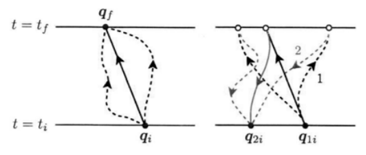
The left schematic shows paths between the initial \mathbf{q}(t_i) and final \mathbf{q}(t_f) times for conservative mechanics. The solid line designates the path for which the action is stationary, while the dashed lines represent the varied paths. The right schematic shows the paths applied to t… — Figure 9.2.2:The left schematic shows paths between the initial $\mathbf{q}(t_i)$ and final $\mathbf{q}(t_f)$ times for conservative mechanics. The solid line designates the path for which the action is stationary, while the dashed lines represent the varied paths. The right schematic shows the paths applied to the doubled degrees of freedom with two initial boundary conditions, that is, $\mathbf{q}_1 (t_i)$ and $\mathbf{q}_2 (t_f)$ plus assuming that both paths are identical at their intersection and that they intersect at the same final time, that is, $\mathbf{q}_1 (t_f) = \mathbf{q}_2 (t_f)$ .

The following describes the framework proposed by Galley for transforming Hamilton’s Principle to a time-asymmetric form. Let $\mathbf{q}$ and $\mathbf{\dot{q}}$ designate sets of $N$ generalized coordinates, plus their velocities, where $\mathbf{q}$ and $\mathbf{\dot{q}}$ are the fundamental variables assumed in the definition of the Lagrangian used by Hamilton’s Principle. As illustrated schematically in Figure 9.2.2, Galley proposed doubling the number of degrees of freedom for the system considered, that is, let $\mathbf{q\rightarrow }\left( \mathbf{q}_{1}\mathbf{,q}_{2}\right)$ and $\mathbf{\dot{q}\rightarrow }\left( \mathbf{\dot{q}}_{1}\mathbf{,\dot{q}} _{2}\right)$ . In addition he defines two identical variational paths 1 and $2,$ where path 2 is the time reverse of path1. That is, path 1 starts at the initial time $t_{i}$ , and ends at $t_{f}$ , whereas path 2 starts at $t_{f}$ and ends at $t_{i}$ . That is, he assumes that $\mathbf{q}$ and $\mathbf{\dot{q}}$ specify the two paths in the space of the doubled degrees of freedom that are identical, and that they intersect at the final time $t_{f}$ . The arrows shown on the paths in Figure 9.2.2 designate the assumed direction of the time integration along these paths.

For the doubled system of degrees of freedom, the total action for the sum of the two paths is given by the time integral of the doubled variables, $S( \mathbf{q}_{1},\mathbf{q}_{2})$ which can be written as

S\left( \mathbf{q}_{1},\mathbf{q}_{2}\right) =\int_{t_{i}}^{t_{f}}L\left( \mathbf{q}_{1},\mathbf{\dot{q}}_{1}\mathbf{,}t\right) dt+\int_{t_{f}}^{t_{i}}L\left( \mathbf{q}_{2},\mathbf{\dot{q}}_{2},t\right) dt=\int_{t_{i}}^{t_{f}}\left[ L\left( \mathbf{q}_{1},\mathbf{\dot{q}}_{1} \mathbf{,}t\right) dt-L\left( \mathbf{q}_{2},\mathbf{\dot{q}}_{2}\mathbf{,} t\right) \right] dt\tag{9.28}

The above relation assumes that the doubled variables $\left( \mathbf{q}_{1}, \mathbf{\dot{q}}_{1}\right)$ and $\left( \mathbf{q}_{2},\mathbf{\dot{q}} _{2}\right)$ are decoupled from each other. More generally one can assume that the two sets of variables are coupled by some arbitrary function $K\left( \mathbf{q}_{1},\mathbf{\dot{q}}_{1},\mathbf{q}_{2},\mathbf{\dot{q}} _{2},t\right)$ . Then the action can be written as

S\left( \mathbf{q}_{1},\mathbf{q}_{2}\right) =\int_{t_{i}}^{t_{f}}\left[ L\left( \mathbf{q}_{1},\mathbf{\dot{q}}_{1}\mathbf{,t}\right) dt-L\left( \mathbf{q}_{2},\mathbf{\dot{q}}_{2}\mathbf{,t}\right) +K\left( \mathbf{q} _{1},\mathbf{\dot{q}}_{1},\mathbf{q}_{2},\mathbf{\dot{q}}_{2},t\right) \right] dt\tag{9.29}

The effective Lagrangian for this doubled system then can be defined as

\Lambda \left( \mathbf{q}_{1},\mathbf{q}_{2},\mathbf{\dot{q}}_{1},\mathbf{ \dot{q}}_{2},t\right) \equiv \left[ L\left( \mathbf{q}_{1},\mathbf{\dot{q}} _{1}\mathbf{,}t\right) dt-L\left( \mathbf{q}_{2},\mathbf{\dot{q}}_{2}\mathbf{ ,}t\right) +K\left( \mathbf{q}_{1},\mathbf{\dot{q}}_{1},\mathbf{q}_{2}, \mathbf{\dot{q}}_{2},t\right) \right]\tag{9.30}

and the action can be written as

S\left( \mathbf{q}_{1},\mathbf{q}_{2}\right) =\int_{t_{i}}^{t_{f}}\Lambda \left( \mathbf{q}_{1},\mathbf{\dot{q}}_{1},\mathbf{q}_{2},\mathbf{\dot{q}} _{2},t\right) dt\tag{9.31}

The coupling term $K\left( \mathbf{q}_{1},\mathbf{\dot{q}}_{1},\mathbf{q} _{2},\mathbf{\dot{q}}_{2},t\right)$ for the doubled system of degrees of freedom must satisfy the following two properties.

(a) If it can be expressed as the difference of two scalar potentials, $\Delta U\left( \mathbf{q}_{1},\mathbf{q}_{2}\right) =U\left( \mathbf{q} _{1}\right) -U\left( \mathbf{q}_{2}\right)$ , then it can be absorbed into the potential term for each of the doubled variables in the Lagrangian. This implies that $K=0,$ and there is no reason to double the number of degrees of freedom because the system is conservative. Thus $K$ describes generalized forces that are not derivable from potential energy, that is, conservative.

(b) A second property of the coupling term $K\left( \mathbf{q}_{1},\mathbf{ \dot{q}}_{1},\mathbf{q}_{2},\mathbf{\dot{q}}_{2},t\right)$ is that it must be antisymmetric under interchange of the arbitrary labels $1\leftrightarrow 2$ . That is,

K\left( \mathbf{q}_{2},\mathbf{\dot{q}}_{2},\mathbf{q}_{1},\mathbf{\dot{q}} _{1},t\right) =-K\left( \mathbf{q}_{1},\mathbf{\dot{q}}_{1},\mathbf{q}_{2}, \mathbf{\dot{q}}_{2},t\right)\tag{9.32}

Therefore the antisymmetric function $K\left( \mathbf{q}_{1},\mathbf{\dot{q}} _{1},\mathbf{q}_{2},\mathbf{\dot{q}}_{2},t\right)$ vanishes when $\mathbf{q} _{2}=\mathbf{q}_{1}$ .

The variational condition requires that the action $S\left( \mathbf{q}_{1}, \mathbf{q}_{2}\right)$ has a well defined stationary point for the doubled system. This is achieved by parametrizing both coordinate paths as

\mathbf{q}_{1,2}(t,\epsilon )=\mathbf{q}_{1,2}(t,0)+\epsilon \eta _{1,2}(t)\tag{9.33}

where $\mathbf{q}_{1,2}(t,0)$ are the coordinates for which the action is stationary, $\epsilon \ll 1.$ and where $\eta _{1,2}(t)$ are arbitrary functions of time denoting virtual displacements of the paths. The doubled system has two independent paths connecting the two initial boundary conditions at $t_{i}$ , and it requires that these paths intersect at $t_{f}$ . The variational system for the two intersecting paths requires specifying four conditions, two per path. Two of the four conditions are determined by requiring that at $t_{i}$ the initial boundary conditions satisfies that $\eta _{1,2}(t_{i})=0$ . The remaining two conditions are derived by requiring that the variation of the action $S\left( \mathbf{q}_{1},\mathbf{q} _{2}\right)$ satisfies

\left[ \frac{dS}{d\epsilon }\right] _{\epsilon =0}=0=\int_{t_{i}}^{t_{f}}dt\left\{ \eta _{1}\left[ \frac{\partial \Lambda }{ \partial q_{1}}-\frac{d\pi _{1}}{dt}\right] _{\epsilon =0}-\eta _{2}\left[ \frac{\partial \Lambda }{\partial q_{2}}-\frac{d\pi _{2}}{dt}\right] _{\epsilon =0}\right\} +\left[ \eta _{1}\pi _{1}-\eta _{2}\pi _{2}\right] _{t=t_{f}}\tag{9.34}

The canonical momenta $\pi _{1,2}$ conjugate to the doubled coordinates $\mathbf{q}_{1,2}$ are defined using the nonconservative Lagrangian $\Lambda$ to be

\pi _{1}^{I}\left( \mathbf{q}_{1,2},\mathbf{\dot{q}}_{1,2}\right) \equiv \frac{\partial \Lambda }{\partial \dot{q}_{1}^{I}(t)}=\frac{\partial L\left( \mathbf{q}_{1},\mathbf{\dot{q}}_{1}\mathbf{,}t\right) }{\partial \dot{q} _{1}^{I}(t)}+\frac{\partial K\left( \mathbf{q}_{1},\mathbf{\dot{q}}_{1}, \mathbf{q}_{2},\mathbf{\dot{q}}_{2},t\right) }{\partial \dot{q}_{1}^{I}(t)}\tag{9.35}

where the superscript $I$ designates the solution based on the initial conditions. Note that the conjugate momentum $p_{1}^{I}=\frac{\partial L\left( \mathbf{q}_{1},\mathbf{\dot{q}}_{1}\mathbf{,}t\right) }{\partial \dot{q}_{1}^{I}(t)}$ while the $\frac{\partial K\left( \mathbf{q}_{1}, \mathbf{\dot{q}}_{1},\mathbf{q}_{2},\mathbf{\dot{q}}_{2},t\right) }{\partial \dot{q}_{1}^{I}(t)}$ term is part of the total momentum due to the nonconservative interaction. Similarly the momentum for the second path is

\pi _{2}^{I}\left( \mathbf{q}_{1,2},\mathbf{\dot{q}}_{1,2}\right) \equiv \frac{\partial \Lambda }{\partial \dot{q}_{2}^{I}(t)}=\frac{\partial L\left( \mathbf{q}_{1},\mathbf{\dot{q}}_{1}\mathbf{,}t\right) }{\partial \dot{q} _{2}^{I}(t)}+\frac{\partial K\left( \mathbf{q}_{1},\mathbf{\dot{q}}_{1}, \mathbf{q}_{2},\mathbf{\dot{q}}_{2},t\right) }{\partial \dot{q}_{2}^{I}(t)}\tag{9.36}

The last term in Equation 9.34, that is, the term $\left[ \eta _{1}\pi _{1}-\eta _{2}\pi _{2}\right] _{t=t_{f}}$ results from integration by parts, which will vanish if

\eta _{1}^{I}(t_{f})\pi _{1}^{I}(t_{f})=\eta _{2}^{I}(t_{f})\pi _{2}^{I}(t_{f})\tag{9.37}

The equality condition at the intersection of the two paths at $t_{f}$ requires that

\eta _{1}^{I}(t_{f})=\eta _{2}^{I}(t_{f})\tag{9.38}

Therefore equations 9.37 and 9.38 imply that

\pi _{1}^{I}(t_{f})=\pi _{2}^{I}(t_{f})\tag{9.39}

Therefore equations 9.38 and 9.39 constitute the equality condition that must be satisfied when the two paths intersect at $t_{f}$ . The equality condition ensures that the boundary term for integration by parts in Equation 9.34 will vanish for arbitrary variations provided that the two unspecified paths agree at the final time $t_{f}$ . Similarly the conjugate momenta $\pi _{1}^{I}(t_{f}),\pi _{2}^{I}(t_{f})$ must agree, but otherwise are unspecified. As a consequence, the equality condition ensures that the variational principle is consistent with the final state at $t_{f}$ not being specified. That is, the equations of motion are only specified by the initial boundary conditions of the time-asymmetric action for the doubled system.

More physics insight is provided by using a more convenient parametrization of the coordinates in terms of their average and difference. That is, let

q_{+}^{I}\equiv \frac{q_{1}^{I}+q_{2}^{I}}{2}\hspace{0.85in}q_{-}^{I}\equiv q_{1}^{I}-q_{2}^{I}\tag{9.40}

Then the physical limit is

q_{+}^{I}\rightarrow q^{I}\hspace{0.85in}q_{-}^{I}\rightarrow 0\tag{9.41}

That is, the average history is the relevant physical history, while the difference coordinate simply vanishes. For these coordinates, the nonconservative Lagrangian is $\Lambda \left( \mathbf{q}_{+},\mathbf{q}_{-}, \mathbf{\dot{q}}_{+},\mathbf{\dot{q}}_{-},t\right)$ and the equality conditions reduce to

\begin{align} \pi _{-}(t_{f}) &=&0 \tag{9.42} \\ \eta _{-}(t_{f}) &=&0 \tag{9.43} \end{align}

which implies that the physically relevant average $\left( +\right)$ quantities are not specified at the final time $t_{f}$ in order to have a well-defined variational principle.

The canonical momenta are given by

\begin{align} \tag{9.44} \pi _{+}^{I} &=&\frac{\pi _{1}^{I}+\pi _{2}^{I}}{2}=\frac{\partial \Lambda }{ \partial \dot{q}_{-}^{I}} \\ \pi _{-}^{I} &=&\pi _{1}^{I}-\pi _{2}^{I}=\frac{\partial \Lambda }{\partial \dot{q}_{+}^{I}}\tag{9.45} \end{align}

The equations of motion can be written as.

\frac{d}{dt}\frac{\partial \Lambda }{\partial \dot{q}_{\pm }^{I}}=\frac{ \partial \Lambda }{\partial q_{\pm }^{I}}\tag{9.46}

Equation 9.46 is identically zero for the $+$ subscript, while, in the physical limit (PL), the negative subscript gives that

\left[ \frac{d}{dt}\frac{\partial \Lambda }{\partial \dot{q}_{-}^{I}}-\frac{ \partial \Lambda }{\partial q_{-}^{I}}\right] _{PL}=0\tag{9.47}

Substituting for the Lagrangian $\Lambda$ gives that

\frac{d}{dt}\frac{\partial L}{\partial \dot{q}_{-}^{I}}-\frac{\partial L}{ \partial q_{-}^{I}}=\left[ \frac{\partial K}{\partial q_{-}^{I}}-\frac{d}{dt} \frac{\partial K}{\partial \dot{q}_{-}^{I}}\right] _{PL}\equiv Q^{I}\left( \mathbf{q}_{1},\mathbf{\dot{q}}_{1}\mathbf{,}t\right)\tag{9.48}

where $Q^{I}$ is a generalized nonconservative force derived from $K$ .

Note that Equation 9.46 can be derived equally well by taking the direct functional derivative with respect to $q_{-}^{I}(t)$ , that is,

0=\left[ \frac{\delta S}{\delta q_{-}^{I}(t)}\right] _{PL}\tag{9.49}

The above time-asymmetric formalism applies Hamilton’s action principle to systems that involve initial boundary conditions while the second path corresponds to the final boundary conditions. This framework, proposed recently by Galley, provides a remarkable advance for the handling of nonconservative action in Lagrangian and Hamiltonian mechanics.^[2] This formalism directly incorporates the variational principle for initial boundary conditions and causal dynamics that are usually required for applications of Lagrangian and Hamiltonian mechanics. Currently, there is limited exploitation of this new formalism because there has been insufficient time for it to become well known, for full recognition of its importance, and for the development and publication of applications. Chapter 10 discusses an application of this formalism to nonconservative systems in classical mechanics.

9.3: Lagrangian¶

Standard Lagrangian¶

Lagrangian mechanics, as introduced in chapter $6,$ was based on the concepts of kinetic energy and potential energy. d’Alembert’s principle of virtual work was used to derive Lagrangian mechanics in chapter 6 and this led to the definition of the standard Lagrangian. That is, the standard Lagrangian was defined in chapter 6.2 to be the difference between the kinetic and potential energies.

L(\mathbf{q, \dot{q},}t)=T(\mathbf{\dot{q},}t)-U(\mathbf{q},t)

Hamilton extended Lagrangian mechanics by defining Hamilton’s Principle, equation $(9.1.2)$ , which states that a dynamical system follows a path for which the action functional is stationary, that is, the time integral of the Lagrangian. Chapter 6 showed that using the standard Lagrangian for defining the action functional leads to the Euler-Lagrange variational equations

\left\{ \frac{d}{dt}\left( \frac{\partial L}{\partial \dot{q}_{j}}\right) - \frac{\partial L}{\partial q_{j}}\right\} =Q_{j}^{EXC}+\sum_{k=1}^{m}\lambda _{k}\frac{\partial g_{k}}{\partial q_{j}}(\mathbf{q},t) \tag{9.51}

The Lagrange multiplier terms handle the holonomic constraint forces and $Q_{j}^{EXC}$ handles the remaining excluded generalized forces. Chapters $6-8$ showed that the use of the standard Lagrangian, with the Euler-Lagrange equations 9.51, provides a remarkably powerful and flexible way to derive second-order equations of motion for dynamical systems in classical mechanics.

Note that the Euler-Lagrange equations, expressed solely in terms of the standard Lagrangian 9.51, that is, excluding the $Q_{j}^{EXC}+ \sum_{k=1}^{m}\lambda _{k}\frac{\partial g_{k}}{\partial q_{j}}(\mathbf{q} ,t)$ terms, are valid only under the following conditions:

The forces acting on the system, apart from any forces of constraint, must be derivable from scalar potentials.
The equations of constraint must be relations that connect the coordinates of the particles and may be functions of time, that is, the constraints are holonomic.

The $Q_{j}^{EXC}+\sum_{k=1}^{m}\lambda _{k}\frac{\partial g_{k}}{ \partial q_{j}}(\mathbf{q},t)$ terms extend the range of validity of using the standard Lagrangian in the Lagrange-Euler equations by introducing constraint and omitted forces explicitly.

Chapters $6-8$ exploited Lagrangian mechanics based on use of the standard definition of the Lagrangian. The present chapter will show that the powerful Lagrangian formulation, using the standard Lagrangian, can be extended to include alternative non-standard Lagrangians that may be applied to dynamical systems where use of the standard definition of the Lagrangian is inapplicable. If these non-standard Lagrangians satisfy Hamilton’s Action Principle, $(9.1.2)$ , then they can be used with the Euler-Lagrange equations to generate the correct equations of motion, even though the Lagrangian may not have the simple relation to the kinetic and potential energies adopted by the standard Lagrangian. Currently, the development and exploitation of non-standard Lagrangians is an active field of Lagrangian mechanics.

Gauge invariance of the standard Lagrangian¶

Note that the standard Lagrangian is not unique in that there is a continuous spectrum of equivalent standard Lagrangians that all lead to identical equations of motion. This is because the Lagrangian $L$ is a scalar quantity that is invariant with respect to coordinate transformations. The following transformations change the standard Lagrangian, but leave the equations of motion unchanged.

The Lagrangian is indefinite with respect to addition of a constant to the scalar potential which cancels out when the derivatives in the Euler-Lagrange differential equations are applied.
The Lagrangian is indefinite with respect to addition of a constant kinetic energy.
The Lagrangian is indefinite with respect to addition of a total time derivative of the form $L_{2}\rightarrow L_{1}+ \frac{d}{dt}\left[ \Lambda (q_{i},t)\right] ,$ for any differentiable function $\Lambda (q_{i}t)$ of the generalized coordinates plus time, that has continuous second derivatives.

This last statement can be proved by considering a transformation between two related standard Lagrangians of the form

\tag{9.52} L_{2}(\mathbf{q},\overset{.}{q},t)=L_{1}(\mathbf{q},\overset{.}{q},t)+\frac{ d\Lambda (\mathbf{q},t)}{dt}=L_{1}(\mathbf{q},\overset{.}{q},t)+\left( \frac{ \partial \Lambda (\mathbf{q},t)}{\partial q_{j}}\dot{q}_{j}+\frac{\partial \Lambda (\mathbf{q},t)}{\partial t}\right)

This leads to a standard Lagrangian $L_{2}$ that has the same equations of motion as $L_{1}$ as is shown by substituting Equation 9.52 into the Euler-Lagrange equations. That is,

\begin{align} \tag{9.53} \frac{d}{dt}\left( \frac{\partial L_{2}}{\partial \dot{q}_{j}}\right) -\frac{ \partial L_{2}}{\partial q_{j}} &=\frac{d}{dt}\left( \frac{\partial L_{1}}{ \partial \dot{q}_{j}}\right) -\frac{\partial L_{1}}{\partial q_{j}}+\frac{ \partial ^{2}\Lambda (\mathbf{q},t)}{\partial t\partial q_{j}}-\frac{ \partial ^{2}\Lambda (\mathbf{q},t)}{\partial t\partial q_{j}} \\[4pt] &=\frac{d}{dt} \left( \frac{\partial L_{1}}{\partial \dot{q}_{j}}\right) -\frac{\partial L_{1}}{\partial q_{j}} \end{align}

Thus even though the related Lagrangians $L_{1}$ and $L_{2}$ are different, they are completely equivalent in that they generate identical equations of motion.

There is an unlimited range of equivalent standard Lagrangians that all lead to the same equations of motion and satisfy the requirements of the Lagrangian. That is, there is no unique choice among the wide range of equivalent standard Lagrangians expressed in terms of generalized coordinates. This discussion is an example of gauge invariance in physics.

Modern theories in physics describe reality in terms of potential fields. Gauge invariance, which also is called gauge symmetry, is a property of field theory for which different underlying fields lead to identical observable quantities. Well-known examples are the static electric potential field and the gravitational potential field where any arbitrary constant can be added to these scalar potentials with zero impact on the observed static electric field or the observed gravitational field. Gauge theories constrain the laws of physics in that the impact of gauge transformations must cancel out when expressed in terms of the observables. Gauge symmetry plays a crucial role in both classical and quantal manifestations of field theory, e.g. it is the basis of the Standard Model of electroweak and strong interactions.

Equivalent Lagrangians are a clear manifestation of gauge invariance as illustrated by equations 9.52, 9.53 which show that adding any total time derivative of a scalar function $\Lambda (\mathbf{q,}t)$ to the Lagrangian has no observable consequences on the equations of motion. That is, although addition of the total time derivative of the scalar function $\Lambda ( \mathbf{q},t)$ changes the value of the Lagrangian, it does not change the equations of motion for the observables derived using equivalent standard Lagrangians.

For Lagrangian formulations of classical mechanics, the gauge invariance is readily apparent by direct inspection of the Lagrangian.

Example 9.3.1: Gauge invariance in electromagnetism

The scalar electric potential $\Phi$ and the vector potential $A$ fields in electromagnetism are examples of gauge-invariant fields. These electromagnetic-potential fields are not directly observable, that is, the electromagnetic observable quantities are the electric field $E$ and magnetic field $B$ which can be derived from the scalar and vector potential fields $\Phi$ and $A$ . An advantage of using the potential fields is that they reduce the problem from 6 components, 3 each for $E$ and $B,$ to 4 components, one for the scalar field $\Phi$ and 3 for the vector potential $A$ . The Lagrangian for the velocity-dependent Lorentz force, given by equation $(6.10.7)$ , provides an example of gauge invariance. Equations $(6.10.3)$ and $(6.10.5)$ showed that the electric and magnetic fields can be expressed in terms of scalar and vector potentials $\Phi$ and $\mathbf{A}$ by the relations

\mathbf{B}=\boldsymbol{\nabla}\times \mathbf{A}

\mathbf{E}=-\boldsymbol{\nabla}\Phi - \frac{\partial \mathbf{A}}{\partial t}\nonumber

The equations of motion for a charge $q$ in an electromagnetic field can be obtained by using the Lagrangian

L=\frac{1}{2}m\mathbf{v}\cdot \mathbf{v}-q(\Phi -\mathbf{A\cdot v)}\nonumber

Consider the transformations $\left( \mathbf{A,}\Phi \right) \rightarrow \left( \mathbf{A}^{\prime },\Phi ^{\prime }\right)$ in the transformed Lagrangian $L^{\prime }$ where

\mathbf{A}^{\prime }=\mathbf{A}+\nabla \Lambda (\mathbf{r,}t)\nonumber

\Phi ^{\prime }=\Phi -\frac{\partial \Lambda (\mathbf{r,}t)}{\partial t}\nonumber

The transformed Lorentz-force Lagrangian $L^{\prime }$ is related to the original Lorentz-force Lagrangian $L$ by

L^{\prime }=L+q\left[ \mathbf{\dot{r}\cdot }\nabla \Lambda (\mathbf{r,}t)+ \frac{\partial \Lambda (\mathbf{r,}t)}{\partial t}\right] =L+q\frac{d}{dt} \Lambda (\mathbf{r,}t)\nonumber

Note that the additive term $q\frac{d}{dt}\Lambda (\mathbf{r,}t)$ is an exact time differential. Thus the Lagrangian $L^{\prime }$ is gauge invariant implying identical equations of motion are obtained using either of these equivalent Lagrangians.

The force fields $\mathbf{E}$ and $\mathbf{B}$ can be used to show that the above transformation is gauge-invariant. That is,

\begin{align*} \mathbf{E}^{\prime } &=-\boldsymbol{\nabla}\Phi ^{\prime }-\frac{\partial \mathbf{ A}^{\prime }}{\partial t} \\[4pt] &=-\boldsymbol{\nabla}\Phi -\frac{\partial \mathbf{A}}{ \partial t} \\[4pt] &=\mathbf{E} \\[4pt] \mathbf{B}^{\prime } &=\boldsymbol{\nabla}\times \mathbf{A}^{\prime } \\[4pt] &=\boldsymbol{ \nabla }\times \mathbf{A} \\[4pt] &=\mathbf{B} \end{align*}

That is, the additive terms due to the scalar field $\Lambda ( \mathbf{r,}t)$ cancel. Thus the electromagnetic force fields following a gauge-invariant transformation are shown to be identical in agreement with what is inferred directly by inspection of the Lagrangian.

Non-standard Lagrangians¶

The definition of the standard Lagrangian was based on d’Alembert’s differential variational principle. The flexibility and power of Lagrangian mechanics can be extended to a broader range of dynamical systems by employing an extended definition of the Lagrangian that is based on Hamilton’s Principle, equation $(9.1.2)$ . Note that Hamilton’s Principle was introduced 46 years after development of the standard formulation of Lagrangian mechanics. Hamilton’s Principle provides a general definition of the Lagrangian that applies to standard Lagrangians, which are expressed as the difference between the kinetic and potential energies, as well as to non-standard Lagrangians where there may be no clear separation into kinetic and potential energy terms. These non-standard Lagrangians can be used with the Euler-Lagrange equations to generate the correct equations of motion, even though they may have no relation to the kinetic and potential energies. The extended definition of the Lagrangian based on Hamilton’s action functional $(9.1.1)$ can be exploited for developing non-standard definitions of the Lagrangian that may be applied to dynamical systems where use of the standard definition is inapplicable. Non-standard Lagrangians can be equally as useful as the standard Lagrangian for deriving equations of motion for a system. Secondly, non-standard Lagrangians, that have no energy interpretation, are available for deriving the equations of motion for many nonconservative systems. Thirdly, Lagrangians are useful irrespective of how they were derived. For example, they can be used to derive conservation laws or the equations of motion. Coordinate transformations of the Lagrangian is much simpler than that required for transforming the equations of motion. The relativistic Lagrangian defined in chapter 17.6 is a well-known example of a non-standard Lagrangian.

Inverse variational calculus¶

Non-standard Lagrangians and Hamiltonians are not based on the concept of kinetic and potential energies. Therefore, development of non-standard Lagrangians and Hamiltonians require an alternative approach that ensures that they satisfy Hamilton’s Principle, equation $(9.1.2)$ , which underlies the Lagrangian and Hamiltonian formulations. One useful alternative approach is to derive the Lagrangian or Hamiltonian via an inverse variational process based on the assumption that the equations of motion are known. Helmholtz developed the field of inverse variational calculus which plays an important role in development of non-standard Lagrangians. An example of this approach is use of the well-known Lorentz force as the basis for deriving a corresponding Lagrangian to handle systems involving electromagnetic forces. Inverse variational calculus is a branch of mathematics that is beyond the scope of this textbook. The Douglas theorem states that, if the three Helmholtz conditions are satisfied, then there exists a Lagrangian that, when used with the Euler-Lagrange differential equations, leads to the given set of equations of motion. Thus, it will be assumed that the inverse variational calculus technique can be used to derive a Lagrangian from known equations of motion.

9.4: Application of Hamilton’s Action Principle to Mechanics¶

Knowledge of the equations of motion is required to predict the response of a system to any set of initial conditions. Hamilton’s action principle, that is built into Lagrangian and Hamiltonian mechanics, coupled with the availability of a wide arsenal of variational principles and techniques, provides a remarkably powerful and broad approach to deriving the equations of motions required to determine the system response.

As mentioned in the Prologue, derivation of the equations of motion for any system, based on Hamilton’s Action Principle, separates naturally into a hierarchical set of three stages that differ in both sophistication and understanding, as described below.

Action stage: The primary “action stage” employs Hamilton’s Action functional, $S=\int_{t_{i}}^{t_{f}}L(\mathbf{q, \dot{q},}t\mathbf{)}dt$ to derive the Lagrangian and Hamiltonian functionals. This action stage provides the most fundamental and sophisticated level of understanding. It involves specifying all the active degrees of freedom, as well as the interactions involved. Symmetries incorporated at this primary action stage can simplify subsequent use of the Hamiltonian and Lagrangian functionals.
Hamiltonian/Lagrangian stage: The “Hamiltonian/Lagrangian stage” uses the Lagrangian or Hamiltonian functionals, that were derived at the action stage, in order to derive the equations of motion for the system of interest. Symmetries, not already incorporated at the primary action stage, may be included at this secondary stage.
Equations of motion stage: The “equations-of-motion stage” uses the derived equations of motion to solve for the motion of the system subject to a given set of initial boundary conditions. Nonconservative forces, such as dissipative forces, that were not included at the primary and secondary stages, may be added at the equations of motion stage.

Lagrange omitted the action stage when he used d’Alembert’s Principle to derive Lagrangian mechanics. The Newtonian mechanics approach omits both the primary “action” stage, as well as the secondary “Hamiltonian/Lagrangian” stage, since Newton’s Laws of Motion directly specify the “equations-of-motion stage”. Thus these do not exploit the considerable advantages provided by the use of the action, the Lagrangian, and the Hamiltonian. Newtonian mechanics requires that all the active forces be included when deriving the equations of motion, which involves dealing with vector quantities. In Newtonian mechanics, symmetries must be incorporated directly at the equations of motion stage, which is more difficult than when done at the primary “action” stage, or the secondary “Lagrangian/Hamiltonian” stage. The “action” and “Hamiltonian/Lagrangian” stages allow for use of the powerful arsenal of mathematical techniques that have been developed for applying variational principles.

There are considerable advantages to deriving the equations of motion based on Hamilton’s Principle, rather than derive them using Newtonian mechanics. It is significantly easier to use variational principles to handle the scalar functionals, action, Lagrangian, and Hamiltonian, rather than starting at the equationsof-motion stage. For example, utilizing all three stages of algebraic mechanics facilitates accommodating extra degrees of freedom, symmetries, and interactions. The symmetries identified by Noether’s theorem are more easily recognized during the primary “action” and secondary “Hamiltonian/Lagrangian” stages rather than at the subsequent “equations of motion” stage. Approximations made at the “action” stage are easier to implement than at the “equations-of-motion” stage. Constrained motion is much more easily handled at the primary “action”, or secondary “Hamilton/Lagrangian” stages, than at the equations-of-motion stage. An important advantage of using Hamilton’s Action Principle, is that there is a close relationship between action in classical and quantal mechanics, as discussed in chapters 15 and 18. Algebraic principles, that underly analytical mechanics, naturally encompass applications to many branches of modern physics, such as relativistic mechanics, fluid motion, and field theory.

In summary, the use of the single fundamental invariant quantity, action, as described above, provides a powerful and elegant framework, that was developed first for classical mechanics, but now is exploited in a wide range of science, engineering, and economics. An important feature of using the algebraic approach to classical mechanics is the tremendous arsenal of powerful mathematical techniques that have been developed for use of variational calculus applied to Lagrangian and Hamiltonian mechanics. Some of these variational techniques were presented in chapters 6, 7, 8, and 9, while others will be introduced in chapter 15.

9.S: Hamilton’s Action Principle (Summary)¶

The Hamilton’s 1834 publication, introducing both Hamilton’s Principle of Stationary Action and Hamiltonian mechanics, marked the crowning achievements for the development of variational principles in classical mechanics. A fundamental advantage of Hamiltonian mechanics is that it uses the conjugate coordinates $\mathbf{q}$ , $\mathbf{p}$ , plus time $t$ , which is a considerable advantage in most branches of physics and engineering. Compared to Lagrangian mechanics, Hamiltonian mechanics has a significantly broader arsenal of powerful techniques that can be exploited to obtain an analytical solution of the integrals of the motion for complicated systems, as described in chapter 15. In addition, Hamiltonian dynamics provides a means of determining the unknown variables for which the solution assumes a soluble form, and is ideal for study of the fundamental underlying physics in applications to fields such as quantum or statistical physics. As a consequence, Hamiltonian mechanics has become the preeminent variational approach used in modern physics.

This chapter has introduced and discussed Hamilton’s Principle of Stationary Action, which underlies the elegant and remarkably powerful Lagrangian and Hamiltonian representations of algebraic mechanics. The basic concepts employed in algebraic mechanics are summarized below.

Hamilton’s Action Principle¶

As discussed in chapter 9.2, Hamiltonian mechanics is built upon Hamilton’s action functional

S(\mathbf{q},\mathbf{p},t) = \int^{t_f}_{t_i} L(\mathbf{q}, \mathbf{\dot{q}},t)dt \tag{9.1}

Hamilton’s Principle of least action states that

\delta S(\mathbf{q},\mathbf{p},t) = \delta \int^{t_f}_{t_i} L(\mathbf{q}, \mathbf{\dot{q}},t)dt = 0 \tag{9.2}

Generalized momentum $p$ ¶

In chapter 7.2, the generalized (canonical) momentum was defined in terms of the Lagrangian $L$ to be

p_i \equiv \frac{\partial L(\mathbf{q}, \mathbf{\dot{q}},t)}{\partial \dot{q}_i} \tag{7.3}

Chapter 9.2.2 defined the generalized momentum in terms of the action functional $S$ to be

p_j \equiv \frac{\partial S(\mathbf{q}, \mathbf{p},t)}{\partial \dot{q}_j} \tag{9.12}

Generalized energy $h (\mathbf{q},\dot{q},t)$ ¶

Jacobi’s Generalized Energy $h (\mathbf{q},\dot{q},t)$ was defined in Equation 7.37 as

h (\mathbf{q},\dot{q},t) \equiv \sum_j \left( \dot{q}_j \frac{\partial L(\mathbf{q}, \mathbf{\dot{q}},t)}{\partial \dot{q}_j} \right) - L(\mathbf{q}, \mathbf{\dot{q}},t) \tag{7.37}

Hamiltonian function $H(\mathbf{q}, \mathbf{p},t)$ ¶

The Hamiltonian $H(\mathbf{q}, \mathbf{p},t)$ was defined in terms of the generalized energy $h (\mathbf{q},\dot{q},t)$ plus the generalized momentum. That is

H(\mathbf{q}, \mathbf{p},t) \equiv h (\mathbf{q},\dot{q},t) = \sum_j p_j\dot{q}_j - L(\mathbf{q}, \mathbf{\dot{q}},t) = \mathbf{p} \cdot \mathbf{\dot{q}} - L(\mathbf{q}, \mathbf{\dot{q}},t)

where $\mathbf{p}$ , $\mathbf{q}$ correspond to $n$ -dimensional vectors, e.g. $\mathbf{q} \equiv (q_1, q_2, \dots , q_n)$ and the scalar product $\mathbf{p} \cdot \mathbf{\dot{q}} = \sum_i p_i \dot{q}_i$ . Chapter 8.2 used a Legendre transformation to derive this relation between the Hamiltonian and Lagrangian functions. Note that whereas the Lagrangian $L(\mathbf{q},\mathbf{\dot{q}},t)$ is expressed in terms of the coordinates $\mathbf{q}$ , plus conjugate velocities $\mathbf{\dot{q}}$ , the Hamiltonian $H (\mathbf{q}, \mathbf{p}, t)$ is expressed in terms of the coordinates $\mathbf{q}$ plus their conjugate momenta $\mathbf{p}$ . For scleronomic systems, using the standard Lagrangian, in equations $(7.9.4)$ and $(7.6.14)$ , shows that the Hamiltonian simplifies to be equal to the total mechanical energy, that is, $H = T + U$ .

Generalized energy theorem¶

The equations of motion lead to the generalized energy theorem which states that the time dependence of the Hamiltonian is related to the time dependence of the Lagrangian.

\frac{dH (\mathbf{q},\mathbf{p},t)}{dt} = \sum_j \dot{q}_j \left[ Q^{EXC}_j + \sum^{m}_{k=1} \lambda_k \frac{\partial g_k}{\partial q_j} (\mathbf{q},t) \right] - \frac{\partial L(\mathbf{q},\mathbf{\dot{q}},t)}{\partial t} \tag{7.38}

Note that if all the generalized non-potential forces and Lagrange multiplier terms are zero, and if the Lagrangian is not an explicit function of time, then the Hamiltonian is a constant of motion.

Lagrange equations of motion¶

Equation 6.60 gives that the $N$ Lagrange equations of motion are

\left\{ \frac{d}{dt} \left(\frac{\partial L}{\partial \dot{q}_j}\right) - \frac{\partial L}{\partial q_j} \right\} = \sum^m_{k=1} \lambda_k \frac{\partial g_k}{\partial q_j} (\mathbf{q}, t) + Q^{EXC}_j \tag{6.60}

where $j = 1, 2, 3, ....N$ .

Hamilton’s equations of motion¶

Chapter 8.3 showed that a Legendre transform, plus the Lagrange-Euler equations, $(8.3.11, 8.3.12, 8.3.13)$ lead to Hamilton’s equations of motion. Hamilton derived these equations of motion directly from the action functional, as shown in chapter 9.2.

\dot{q}_j = \frac{\partial H (\mathbf{q},\mathbf{p},t)}{ \partial p_j} \tag{8.25}

\begin{align} \dot{p}_j &=& −\frac{\partial H}{\partial q_j} (\mathbf{q},\mathbf{p},t) + \left[ \sum^m_{k=1} \lambda_k \frac{\partial g_k}{\partial q_j} (\mathbf{q}, t) + Q^{EXC}_j \right] \tag{8.26}\end{align}

\frac{\partial H (\mathbf{q},\mathbf{p},t)}{\partial t } = −\frac{\partial L(\mathbf{q},\mathbf{\dot{q}},t)}{\partial t} \tag{8.24}

Note the symmetry of Hamilton’s two canonical equations. The canonical variables $p_k$ , $q_k$ are treated as independent canonical variables. Lagrange was the first to derive the canonical equations but he did not recognize them as a basic set of equations of motion. Hamilton derived the canonical equations of motion from his fundamental variational principle and made them the basis for a far-reaching theory of dynamics. Hamilton’s equations give $2s$ first-order differential equations for $p_k$ , $q_k$ for each of the $s$ degrees of freedom. Lagrange’s equations give $s$ second-order differential equations for the variables $q_k$ , $\dot{q}_k$ .

Hamilton-Jacobi equation¶

Hamilton used Hamilton’s Principle plus Equation 9.19 to derive the Hamilton-Jacobi equation.

\frac{\partial S}{\partial t} + H(\mathbf{q},\mathbf{p},t)=0 \tag{9.19}

The solution of Hamilton’s equations is trivial if the Hamiltonian is a constant of motion, or when a set of generalized coordinate can be identified for which all the coordinates $q_i$ are constant, or are cyclic (also called ignorable coordinates). Jacobi developed the mathematical framework of canonical transformation required to exploit the Hamilton-Jacobi equation.

Hamilton’s Principle applied using initial boundary conditions¶

The definition of Hamilton’s Principle assumes integration between the initial time $t_i$ and final time $t_f$ . A recent development has extended applications of Hamilton’s Principle to apply to systems that are defined in terms of only the initial boundary conditions. This method doubles the number of degrees of freedom and uses a coupling Lagrangian $K (\mathbf{q}_2, \mathbf{\dot{q}}_2, \mathbf{q}_1, \mathbf{\dot{q}}_1, t)$ between the corresponding $\mathbf{q}_1$ and $\mathbf{q}_2$ doubled degrees of freedom

\frac{d}{dt} \frac{ \partial L}{ \partial \dot{q}^I_-} − \frac{\partial L}{\partial q^{I}_-} = \left[ \frac{\partial K}{\partial q^I_-} − \frac{d}{dt} \frac{\partial K}{\partial \dot{q}^I_-} \right]_{PL} \equiv Q^I (\mathbf{q}_1, \mathbf{\dot{q}}_1, t) \tag{9.50}

and where $Q^I$ is a generalized nonconservative force derived from $K$ .

Standard Lagrangians¶

Derivation of Lagrangian mechanics, using d’Alembert’s principle of virtual work, assumed that the Lagrangian is defined by Equation 9.52

L(\mathbf{q}, \mathbf{\dot{q}},t) = T(\mathbf{\dot{q}},t) − U(\mathbf{q}, t) \tag{9.52}

This was used in equation $(9.2.1)$ to derive the action in terms of the fundamental Lagrangian defined by Equation 9.52. The assumption that the action $S$ is the fundamental property inverts this procedure and now equation $(9.2.1)$ is used to derived the Lagrangian. That is, the assumption that Hamilton’s Principle is the foundation of algebraic mechanics defines the Lagrangian in terms of the fundamental action $S$ .

Non-standard Lagrangians¶

The flexibility and power of Lagrangian mechanics can be extended to a broader range of dynamical systems by employing an extended definition of the Lagrangian that assumes that the action is the fundamental property, and then the Lagrangian is defined in terms of Hamilton’s variational action principle using Equation 9.2. It was illustrated that the inverse variational calculus formalism can be used to identify non-standard Lagrangians that generate the required equations of motion. These nonstandard Lagrangians can be very different from the standard Lagrangian and do not separate into kinetic and potential energy components. These alternative Lagrangians can be used to handle dissipative systems which are beyond the range of validity when using standard Lagrangians. That is, it was shown that several very different Lagrangians and Hamiltonians can be equivalent for generating useful equations of motion of a system. Currently the use of non-standard Lagrangians is a narrow, but active, frontier of classical mechanics with important applications to relativistic mechanics.

Gauge invariance of the standard Lagrangian¶

It was shown that there is a continuum of equivalent standard Lagrangians that lead to the same set of equations of motion for a system. This feature is related to gauge invariance in mechanics. The following transformations change the standard Lagrangian, but leave the equations of motion unchanged.

The Lagrangian is indefinite with respect to addition of a constant to the scalar potential which cancels out when the derivatives in the Euler-Lagrange differential equations are applied.
Similarly the Lagrangian is indefinite with respect to addition of a constant kinetic energy.
The Lagrangian is indefinite with respect to addition of a total time derivative of the form $L + \frac { d } { d t } \left[ \Lambda \left( q _ { i } , t \right) \right]$ for any differentiable function $\Lambda \left( q _ { i } t \right)$ of the generalized coordinates, plus time, that has continuous second derivatives.

Application of Hamilton’s Action Principle to mechanics¶

The derivation of the equations of motion for any system can be separated into a hierarchical set of three stages in both sophistication and understanding. Variational principles are employed during the primary “action” stage and secondary “Hamilton/Lagrangian” stage to derive the required equations of motion, which then are solved during the third “equations-of-motion stage”. Hamilton’s Action Principle, is a scalar function that is the basis for deriving the Lagrangian and Hamiltonian functions. The primary “action stage” uses Hamilton’s Action functional, $S = \int^{t_f}_{t_i} L (\mathbf{q},\mathbf{\dot{q}},t) dt$ to derive the Lagrangian and Hamiltonian functionals that are based on Hamilton’s action functional and provide the most fundamental and sophisticated level of understanding. The second “Hamiltonian/Lagrangian stage” involves using the Lagrangian and Hamiltonian functionals to derive the equations of motion. The third “equations-of-motion stage” uses the derived equations of motion to solve for the motion subject to a given set of initial boundary conditions. The Newtonian mechanics approach bypasses the primary “action” stage, as well as the secondary “Hamiltonian/Lagrangian” stage. That is, Newtonian mechanics starts at the third “equations-of-motion” stage, which does not allow exploiting the considerable advantages provided by use of action, the Lagrangian, and the Hamiltonian. Newtonian mechanics requires that all the active forces be included when deriving the equations of motion, which involves dealing with vector quantities. This is in contrast to the action, Lagrangian, and Hamiltonian which are scalar functionals. Both the primary “action” stage, and the secondary “Lagrangian/Hamiltonian” stage, exploit the powerful arsenal of mathematical techniques that have been developed for exploiting variational principles.

Footnotes¶

The term “action functional” was named “Hamilton’s Principal Function” in older texts. The name usually is abbreviated to “action” in modern mechanics.
↩
This topic goes beyond the planned scope of this book. It is recommended that the reader refer to the work of Galley, Tsang, and Stein[Gal13, Gal14] for further discussion plus examples of applying this formalism to nonconservative systems in classical mechanics, electromagnetic radiation, RLC circuits, fluid dynamics, and field theory.
↩