5. Calculus of Variations

5.1: Introduction to the Calculus of Variations¶

During the $18^{th}$ century, Bernoulli, who was a student of Leibniz, developed the field of variational calculus which underlies the integral variational approach to mechanics. He solved the brachistochrone problem which involves finding the path for which the transit time between two points is the shortest. The integral variational approach also underlies Fermat’s principle in optics, which can be used to derive that the angle of reflection equals the angle of incidence, as well as derive Snell’s law. Other applications of the calculus of variations include solving the catenary problem, finding the maximum and minimum distances between two points on a surface, polygon shapes having the maximum ratio of enclosed area to perimeter, or maximizing profit in economics. Bernoulli, developed the principle of virtual work used to describe equilibrium in static systems, and d’Alembert extended the principle of virtual work to dynamical systems. Euler, the preeminent Swiss mathematician of the $18^{th}$ century and a student of Bernoulli, developed the calculus of variations with full mathematical rigor. The culmination of the development of the Lagrangian variational approach to classical mechanics was done by Lagrange (1736-1813), who was a student of Euler.

The Euler-Lagrangian approach to classical mechanics stems from a deep philosophical belief that the laws of nature are based on the principle of economy. That is, the physical universe follows paths through space and time that are based on extrema principles. The standard Lagrangian $L$ is defined as the difference between the kinetic and potential energy, that is

L=T-U

Chapters 6 through 9 will show that the laws of classical mechanics can be expressed in terms of Hamilton’s variational principle which states that the motion of the system between the initial time $t_{1}$ and final time $t_{2}$ follows a path that minimizes the scalar action integral $S$ defined as the time integral of the Lagrangian.

S=\int_{t_{1}}^{t_{2}}Ldt

The calculus of variations provides the mathematics required to determine the path that minimizes the action integral. This variational approach is both elegant and beautiful, and has withstood the rigors of experimental confirmation. In fact, not only is it an exceedingly powerful alternative approach to the intuitive Newtonian approach in classical mechanics, but Hamilton’s variational principle now is recognized to be more fundamental than Newton’s Laws of Motion. The Lagrangian and Hamiltonian variational approaches to mechanics are the only approaches that can handle the Theory of Relativity, statistical mechanics, and the dichotomy of philosophical approaches to quantum physics.

5.2: Euler’s Differential Equation¶

The calculus of variations, presented here, underlies the powerful variational approaches that were developed for classical mechanics. Variational calculus, developed for classical mechanics, now has become an essential approach to many other disciplines in science, engineering, economics, and medicine.

For the special case of one dimension, the calculus of variations reduces to varying the function $y(x)$ such that the scalar functional $F$ is an extremum, that is, it is a maximum or minimum, where.

F=\int_{x_{1}}^{x_{2}}f\left[ y(x),y^{\prime }(x);x\right] dx

Here $x$ is the independent variable, $y(x)$ the dependent variable, plus its first derivative $y^{\prime }\equiv \frac{dy}{dx}$ . The quantity $f\left[ y(x),y^{\prime }(x);x\right]$ has some given dependence on $y,y^{\prime }$ and $x.$ The calculus of variations involves varying the function $y(x)$ until a stationary value of $F$ is found, which is presumed to be an extremum. This means that if a function $y=y(x)$ gives a minimum value for the scalar functional $F$ , then any neighboring function, no matter how close to $y(x),$ must increase $F$ . For all paths, the integral $F$ is taken between two fixed points, $x_{1},y_{1}$ and $x_{2},y_{2}$ . Possible paths between the initial and final points are illustrated in Figure 5.2.1. Relative to any neighboring path, the functional $F$ must have a stationary value which is presumed to be the correct extremum path.

Define a neighboring function using a parametric representation $y(\epsilon ,x),$ such that for $\epsilon =0$ , $y=y(0,x)=y(x)$ is the function that yields the extremum for $F$ . Assume that an infinitesimally small fraction $\epsilon$ of the neighboring function $\eta (x)$ is added to the extremum path $y(x)$ . That is, assume

\begin{align} y(\epsilon ,x) & = y(0,x)+\epsilon \eta (x) \tag{5.4} \\[4pt] y^{\prime }(\epsilon ,x) & \equiv \frac{dy(\epsilon ,x)}{dx}=\frac{dy(0,x)}{ dx}+\epsilon \frac{d\eta }{dx} \notag\end{align}

where it is assumed that the extremum function $y(0,x)$ and the auxiliary function $\eta (x)$ are well behaved functions of $x$ with continuous first derivatives, and where $\eta (x)$ vanishes at $x_{1}$ and $x_{2},$ because, for all possible paths, the function $y(\epsilon ,x)$ must be identical with $y(x)$ at the end points of the path, i.e. $\eta (x_{1})=\eta (x_{2})=0$ . The situation is depicted in Figure 5.2.1. It is possible to express any such parametric family of curves $F$ as a function of $\epsilon$

F(\epsilon )=\int_{x_{1}}^{x_{2}}f\left[ y(\epsilon ,x),y^{\prime }(\epsilon ,x);x\right] dx \tag{5.5}

The condition that the integral has a stationary (extremum) value is that $F$ be independent of $\epsilon$ to first order along the path. That is, the extremum value occurs for ( $\epsilon =0$ ) where

\left( \frac{dF}{d\epsilon }\right) _{\epsilon =0}=0 \tag{5.6}

for all functions $\eta (x).$ This is illustrated on the right side of Figure 5.2.1.

Applying condition 5.6 to Equation 5.5, and since $x$ is independent of $\epsilon ,$ then

\frac{\partial F}{\partial \epsilon }=\int_{x_{1}}^{x_{2}}\left( \frac{ \partial f}{\partial y}\frac{\partial y}{\partial \epsilon }+\frac{\partial f }{\partial y^{\prime }}\frac{\partial y^{\prime }}{\partial \epsilon } \right) dx=0 \tag{5.7}

Since the limits of integration are fixed, the differential operation affects only the integrand. From equations 5.4,

\frac{\partial y}{\partial \epsilon }=\eta (x)

and

\frac{\partial y^{\prime }}{\partial \epsilon }=\frac{d\eta }{dx}

Consider the second term in the integrand

\int_{x_{1}}^{x_{2}}\frac{\partial f}{\partial y^{\prime }}\frac{\partial y^{\prime }}{\partial \epsilon }dx=\int_{x_{1}}^{x_{2}}\frac{\partial f}{ \partial y^{\prime }}\frac{d\eta }{dx}dx

The left shows the extremum y(x) and neighboring paths y(\epsilon, x) = y(x) + \epsilon \eta (x) between (x_1, y_1) and (x_2, y_2) that minimizes the function F = \int^{x_2}_{x_1} f[y(x), y^{\prime}(x); x] dx. The right shows the dependence of F as a function of the admixture coefficient \epsilon… — Figure 5.2.1:The left shows the extremum $y(x)$ and neighboring paths $y(\epsilon, x) = y(x) + \epsilon \eta (x)$ between $(x_1, y_1)$ and $(x_2, y_2)$ that minimizes the function $F = \int^{x_2}_{x_1} f[y(x), y^{\prime}(x); x] dx$ . The right shows the dependence of $F$ as a function of the admixture coefficient $\epsilon$ for a maximum (upper) or a minimum (lower) at $\epsilon = 0$ .

Integrate by parts

\int udv=uv-\int vdu

gives

\int_{x_{1}}^{x_{2}}\frac{\partial f}{\partial y^{\prime }}\frac{d\eta }{dx} dx=\left[ \frac{\partial f}{\partial y^{\prime }}\eta (x)\right] _{x_{1}}^{x_{2}}-\int_{x_{1}}^{x_{2}}\eta (x)\frac{d}{dx}\left( \frac{ \partial f}{\partial y^{\prime }}\right) dx

Note that the first term on the right-hand side is zero since by definition $\frac{\partial y}{\partial \epsilon }=\eta (x)=0$ at $x_{1}$ and $x_{2}.$ Thus

\begin{align*} \frac{\partial F}{\partial \epsilon } &=\int_{x_{1}}^{x_{2}}\left( \frac{ \partial f}{\partial y}\frac{\partial y}{\partial \epsilon }+\frac{\partial f }{\partial y^{\prime }}\frac{\partial y^{\prime }}{\partial \epsilon } \right) dx \\[4pt] &=\int_{x_{1}}^{x_{2}}\left( \frac{\partial f}{\partial y}\eta (x)-\eta (x)\frac{d}{dx}\left( \frac{\partial f}{\partial y^{\prime }} \right) \right) dx \end{align*}

Thus Equation 5.7 reduces to

\frac{\partial F}{\partial \epsilon }=\int_{x_{1}}^{x_{2}}\left( \frac{ \partial f}{\partial y}-\frac{d}{dx}\frac{\partial f}{\partial y^{\prime }} \right) \eta (x)dx

The function $\frac{\partial F}{\partial \epsilon }$ will be an extremum if it is stationary at $\epsilon =0$ . That is,

\frac{\partial F}{\partial \epsilon }=\int_{x_{1}}^{x_{2}}\left( \frac{ \partial f}{\partial y}-\frac{d}{dx}\frac{\partial f}{\partial y^{\prime }} \right) \eta (x)dx=0

This integral now appears to be independent of $\epsilon .$ However, the functions $y$ and $y^{\prime }$ occurring in the derivatives are functions of $\epsilon$ . Since $\left( \frac{\partial F}{\partial \epsilon }\right) _{\epsilon =0}$ must vanish for a stationary value, and because $\eta (x)$ is an arbitrary function subject to the conditions stated ,then the above integrand must be zero. This derivation that the integrand must be zero leads to Euler’s differential equation

\frac{\partial f}{\partial y}-\frac{d}{dx}\frac{\partial f}{\partial y^{\prime }}=0

where $y$ and $y^{\prime }$ are the original functions, independent of $\epsilon$ . The basis of the calculus of variations is that the function $y(x)$ that satisfies Euler’s equation is an stationary function. Note that the stationary value could be either a maximum or a minimum value. When Euler’s equation is applied to mechanical systems using the Lagrangian as the functional, then Euler’s differential equation is called the Euler-Lagrange equation.

5.3: Applications of Euler’s Equation¶

Example 5.3.1: Shortest distance between two points

Consider the path lies in the $\mathit{x-y}$ plane.

Figure 5.3.1:Shortest distance between two points in a plane.

The infinitessimal length of arc is

ds = \sqrt{dx^{2}+dy^{2}} = \left[ \sqrt{1+\left( \frac{dy}{dx}\right) ^{2}}\right] dx\nonumber

Then the length of the arc is

J = \int_{1}^{2}ds = \int_{1}^{2}\left[ \sqrt{1+\left( \frac{dy}{dx}\right) ^{2}} \right] dx\nonumber

The function $f$ is

f = \sqrt{1+\left( y^{\prime }\right) ^{2}}\nonumber

Therefore

\frac{\partial f}{\partial y} = 0\nonumber

and

\frac{\partial f}{\partial y^{\prime }} = \frac{y^{\prime }}{\sqrt{1+\left( y^{\prime }\right) ^{2}}}\nonumber

Inserting these into Euler’s equation $(5.2.13)$ gives

0+\frac{d}{dx}\left( \frac{y^{\prime }}{\sqrt{1+\left( y^{\prime }\right) ^{2}}}\right) = 0\nonumber

that is

\frac{y^{\prime }}{\sqrt{1+\left( y^{\prime }\right) ^{2}}} = \text{constant} = C\nonumber

This is valid if

y^{\prime } = \frac{C}{\sqrt{1-C^{2}}} = a\nonumber

Therefore

y = ax+b\nonumber

which is the equation of a straight line in the plane. Thus the shortest path between two points in a plane is a straight line between these points, as is intuitively obvious. This stationary value obviously is a minimum.

This trivial example of the use of Euler’s equation to determine an extremum value has given the obvious answer. It has been presented here because it provides a proof that a straight line is the shortest distance in a plane and illustrates the power of the calculus of variations to determine extremum paths.

Example 5.3.2: Brachistochrone problem

The Brachistochrone problem involves finding the path having the minimum transit time between two points. The Brachistochrone problem stimulated the development of the calculus of variations by John Bernoulli and Euler. For simplicity, take the case of frictionless motion in the $x-y$ plane with a uniform gravitational field acting in the $\widehat{\mathbf{y}}$ direction, as shown in the adjacent figure. The question is what constrained path will result in the minimum transit time between two points $(x_{1}y_{1})$ and $(x_{2}y_{2}).$

Figure 5.3.2:The Bachistochrone problem involves finding the path for the minimum transit time for constrained frictionless motion in a uniform gravitational field.

Consider that the particle of mass $m$ starts at the origin $x_{1} = 0,y_{1} = 0$ with zero velocity. Since the problem conserves energy and assuming that initially $E = KE+PE = 0$ then

\frac{1}{2}mv^{2}-mgy = 0\nonumber

That is

v = \sqrt{2gy}\nonumber

The transit time is given by

t = \int_{x_{1}}^{x_{2}}\frac{ds}{v} = \int_{x_{1}}^{x_{2}}\frac{\sqrt{ dx^{2}+dy^{2}}}{\sqrt{2gy}} = \int_{x_{1}}^{x_{2}}\sqrt{\frac{\left( 1+x^{\prime 2}\right) }{2gy}}dy\nonumber

where $x^{\prime }\equiv \frac{dx}{dy}$ . Note that, in this example, the independent variable has been chosen to be $y$ and the dependent variable is $x(y)$ .

The function $f$ of the integral is

f = \frac{1}{\sqrt{2g}}\sqrt{\frac{\left( 1+x^{\prime 2}\right) }{y}}\nonumber

Factor out the constant $\sqrt{2g}$ term, which does not affect the final equation, and note that

\begin{aligned} \frac{\partial f}{\partial x} & = &0 \\ \frac{\partial f}{\partial x^{\prime }} & = &\frac{x^{\prime }}{\sqrt{y\left( 1+\left( x^{\prime }\right) ^{2}\right) }}\end{aligned}\nonumber

Therefore Euler’s equation gives

0+\frac{d}{dy}\left( \frac{x^{\prime }}{\sqrt{y\left( 1+\left( x^{\prime }\right) ^{2}\right) }}\right) = 0\nonumber

\frac{x^{\prime }}{\sqrt{y\left( 1+\left( x^{\prime }\right) ^{2}\right) }} = \text{constant} = \frac{1}{\sqrt{2a}}\nonumber

That is

\frac{x^{\prime 2}}{y\left( 1+\left( x^{\prime }\right) ^{2}\right) } = \frac{1 }{2a}\nonumber

This may be rewritten as

x = \int_{y_{1}}^{y_{2}}\frac{ydy}{\sqrt{2ay-y^{2}}}\nonumber

Change the variable to $y = a(1-\cos \theta )$ gives that $dy = a\sin \theta d\theta ,$ leading to the integral

x = \int a\left( 1-\cos \theta \right) d\theta\nonumber

x = a(\theta -\sin \theta )+\text{constant}\nonumber

The parametric equations for a cycloid passing through the origin are

\begin{aligned} x & = &a(\theta -\sin \theta ) \\ y & = &a(1-\cos \theta )\end{aligned}\nonumber

which is the form of the solution found. That is, the shortest time between two points is obtained by constraining the motion of the mass to follow a cycloid shape. Thus the mass first accelerates rapidly by falling down steeply and then follows the curve and coasts upward at the end. The elapsed time is obtained by inserting the above parametric relations for $x$ and $y,$ in terms of $\theta ,$ into the transit time integral giving $t = \sqrt{\frac{a}{g}}\theta$ where $\ a$ and $\theta$ are fixed by the end point coordinates. Thus the time to fall from starting with zero velocity at the cusp to the minimum of the cycloid is $\pi \sqrt{\frac{a}{g}}.$ If $y_{2} = y_{1} = 0$ then $x_{2} = 2\pi a$ which defines the shape of the cycloid and the minimum time is $2\pi \sqrt{\frac{a}{g}} = \sqrt{ \frac{2\pi x_{2}}{g}}.$ If the mass starts with a non-zero initial velocity, then the starting point is not at the cusp of the cycloid, but down a distance $d$ such that the kinetic energy equals the potential energy difference from the cusp.

A modern application of the Brachistochrone problem is determination of the optimum shape of the low-friction emergency chute that passengers slide down to evacuate a burning aircraft. Bernoulli solved the problem of rapid evacuation of an aircraft two centuries before the first flight of a powered aircraft.

Example 5.3.3: Minimal travel cost

Assume that the cost of flying an aircraft at height $z$ is $e^{-\kappa z}$ per unit distance of flight-path, where $\kappa$ is a positive constant. Consider that the aircraft flies in the $(x,z)$ -plane from the point $(-a,0)$ to the point $(a,0)$ where $z = 0$ corresponds to ground level, and where the $z$ -axis points vertically upwards. Find the extremal for the problem of minimizing the total cost of the journey.

The differential arc-length element of the flight path $ds$ can be written as

ds = \sqrt{dx^{2}+dz^{2}} = \sqrt{1+z^{\prime 2}}dx\nonumber

where $z^{\prime }\equiv \frac{dz}{dx}$ . Thus the cost integral to be minimized is

C = \int_{-a}^{+a}e^{-\kappa z}ds = \int_{-a}^{+a}e^{-\kappa z}\sqrt{1+z^{\prime 2}}dx\nonumber

The function of this integral is

f = e^{-\kappa z}\sqrt{1+z^{\prime 2}}\nonumber

The partial differentials required for the Euler equations are

\begin{aligned} \frac{d}{dx}\frac{\partial f}{\partial z^{\prime }} & = &\frac{z^{\prime \prime }e^{-\kappa z}}{\sqrt{1+z^{\prime 2}}}-\frac{\kappa z^{\prime 2}e^{-\kappa z}}{\sqrt{1+z^{\prime 2}}}-\frac{z^{\prime \prime }z^{\prime 2}e^{-\kappa z}}{\left( 1+z^{\prime 2}\right) ^{3/2}} \\ \frac{\partial f}{\partial z} & = &-\kappa e^{-\kappa z}\sqrt{1+z^{\prime 2}}\end{aligned}\nonumber

Therefore Euler’s equation equals

\frac{\partial f}{\partial z}-\frac{d}{dx}\frac{\partial f}{\partial z^{\prime }} = -\kappa e^{-\kappa z}\sqrt{1+z^{\prime 2}}-\frac{z^{\prime \prime }e^{-\kappa z}}{\sqrt{1+z^{\prime 2}}}+\frac{\kappa z^{\prime 2}e^{-\kappa z}}{\sqrt{1+z^{\prime 2}}}+\frac{z^{\prime \prime }z^{\prime 2}e^{-\kappa z}}{\left( 1+z^{\prime 2}\right) ^{3/2}} = 0\nonumber

This can be simplified by multiplying the radical to give

-\kappa -2\kappa z^{\prime 2}-\kappa z^{\prime 4}-z^{\prime \prime }-z^{\prime \prime }z^{\prime 2}+\kappa z^{\prime 2}+\kappa z^{\prime 4}+z^{\prime \prime }z^{\prime 2} = 0\nonumber

Cancelling terms gives

z^{\prime \prime }+\kappa \left( 1+z^{\prime 2}\right) = 0\nonumber

Separating the variables leads to

\arctan z^{\prime } = \int \frac{dz^{\prime }}{z^{\prime 2}+1} = -\int \kappa dx = -\kappa z+c_{1}\nonumber

Integration gives

z(x) = \int_{-a}^{x}dz = \int_{-a}^{x}\tan (c_{1}-\kappa x)dx = \frac{\ln (\cos (c_{1}-\kappa x))-\ln (\cos (c_{1}+\kappa a))}{\kappa }+c_{2} = \frac{\ln \left( \frac{\cos (c_{1}-\kappa x)}{\cos (c_{1}+\kappa a)}\right) }{\kappa } +c_{2}\nonumber

Using the initial condition that $z(-a) = 0$ gives $c_{2} = 0$ . Similarly the final condition $z(a) = 0$ implies that $c_{1} = 0$ . Thus Euler’s equation has determined that the optimal trajectory that minimizes the cost integral $C$ is

z(x) = \frac{1}{\kappa }\ln \left( \frac{\cos (\kappa x)}{\cos (\kappa a)} \right)\nonumber

This example is typical of problems encountered in economics.

5.4: Selection of the Independent Variable¶

A wide selection of variables can be chosen as the independent variable for variational calculus. The derivation of Euler’s equation and example (5.3.1) both assumed that the independent variable is $x,$ whereas example (5.3.2) used $y$ as the independent variable, example (5.3.3) used $z$ , and Lagrange mechanics uses time $t$ as the independent variable. Selection of which variable to use as the independent variable does not change the physics of a problem, but some selections can simplify the mathematics for obtaining an analytic solution. The following example of a cylindrically-symmetric soap-bubble surface formed by blowing a soap bubble that stretches between two circular hoops, illustrates the importance when selecting the independent variable.

Example 5.4.1: Surface area of a cylindrically-symmetric soap bubble

Consider a cylindrically-symmetric soap-bubble surface formed by blowing a soap bubble that stretches between two circular hoops. The surface energy, that results from the surface tension of the soap bubble, is minimized when the surface area of the bubble is minimized. Assume that the axes of the two hoops lie along the $z$ axis as shown in the adjacent figure. It is intuitively obvious that the soap bubble having the minimum surface area that is bounded by the two hoops will have a circular cross section that is concentric with the symmetry axis, and the radius will be smaller between the two hoops. Therefore, intuition can be used to simplify the problem to finding the shape of the contour of revolution around the axis of symmetry that defines the shape of the surface of minimum surface area. Use cylindrical coordinates $(\rho ,\theta ,z)$ and assume that hoop 1 at $z_{1}$ has radius $\rho _{1}$ and hoop 2 at $z_{2}$ has radius $\rho _{2}$ . Consider the cases where either $\rho$ , or $z$ , are selected to be the independent variable.

Figure 5.4.1:Cylindrically-symmetric surface formed by rotation about the $z$ axis of a soap bubble suspended between two identical hoops centred on the $z$ axis.

The differential arc-length element of the circular annulus at constant $\theta$ between $z$ and $z+dz$ is given by $ds=\sqrt{dz^{2}+d\rho ^{2}}$ . Therefore the area of the infinitessimal circular annulus is $dS=2\pi \rho ds$ which can be integrated to give the area of the surface $S$ of the soap bubble bounded by the two circular hoops as

S=2\pi \int_{1}^{2}\rho \sqrt{dz^{2}+d\rho ^{2}}\nonumber

Independent variable $z$

\frac{d}{dz}\left( \frac{\rho \rho ^{\prime }}{\sqrt{1+\left( \rho ^{\prime }\right) ^{2}}}\right) -\sqrt{1+\rho ^{\prime 2}}=0\nonumber

This is not an easy equation to solve.

Independent variable $\rho$

\rho =a\cosh \frac{z-b}{a}\nonumber

which is the equation of a catenary. The catenary is the shape of a uniform flexible cable hung in a uniform gravitational field. The constants $a$ and $b$ are given by the end points. The physics of the solution must be identical for either choice of independent variable. However, mathematically one case is easier to solve than the other because, in the latter case, one term in Euler’s equation is zero.

5.5: Functions with Several Independent Variables¶

Functions with several independent variables $y_{i}(x)$ ¶

The discussion has focussed on systems having only a single function $y(x)$ such that the functional is an extremum. It is more common to have a functional that is dependent upon several independent variables $f\left[ y_{1}(x),y_{1}^{\prime }(x),y_{2}(x),y_{2}^{\prime }(x),....;x\right]$ which can be written as

F=\int_{x_{1}}^{x_{2}}\sum_{i=1}^{N}f\left[ y_{i}(x),y_{i}^{\prime }(x);x \right] dx

where $i=1,2,3,....,N.$

By analogy with the one dimensional problem, define neighboring functions $\eta _{i}$ for each variable. Then

\begin{align} y_{i}(\epsilon ,x) &=&y_{i}(0,x)+\epsilon \eta _{i}(x) \tag{5.17} \\ y_{i}^{\prime }(\epsilon ,x) &\equiv &\frac{dy_{i}(\epsilon ,x)}{dx}=\frac{ dy_{i}(0,x)}{dx}+\epsilon \frac{d\eta _{i}}{dx} \notag\end{align}

where $\eta _{i}$ are independent functions of $x$ that vanish at $x_{1}$ and $x_{2}.$ Using equations (5.2.10) and 5.17 leads to the requirements for an extremum value to be

\frac{\partial F}{\partial \epsilon }=\int_{x_{1}}^{x_{2}}\sum_{i}^{N}\left( \frac{\partial f}{\partial y_{i}}\frac{\partial y_{i}}{\partial \epsilon }+\frac{\partial f}{\partial y_{i}^{\prime }}\frac{\partial y_{i}^{\prime }}{ \partial \epsilon }\right) dx=\int_{x_{1}}^{x_{2}}\sum_{i}^{N}\left( \frac{ \partial f}{\partial y_{i}}-\frac{d}{dx}\frac{\partial f}{\partial y_{i}^{\prime }}\right) \eta _{i}(x)dx=0

If the variables $y_{i}(x)$ are independent, then the $\eta _{i}(x)$ are independent. Since the $\eta _{i}(x)$ are independent, then evaluating the above equation at $\epsilon =0$ implies that each term in the bracket must vanish independently. That is, Euler’s differential equation becomes a set of $N$ equations for the $N$ independent variables

\frac{\partial f}{\partial y_{i}}-\frac{d}{dx}\frac{\partial f}{\partial y_{i}^{\prime }}=0

where $i=1,2,3..N.$ Thus, each of the $N$ equations can be solved independently when the $N$ variables are independent. Euler’s equation involves partial derivatives for the dependent variables $y_{i}$ , $y_{i\text{ }}^{\prime }$ and the total derivative for the independent variable $x$ .

Example 5.5.1: Fermat’s Principle

In $\mathit{1662}$ Fermat’s proposed that the propagation of light obeyed the generalized principle of least transit time. In optics, Fermat’s principle, or the principle of least time, is the principle that the path taken between two points by a ray of light is the path that can be traversed in the least time. Historically, the proof of Fermat’s principle by Johann Bernoulli was one of the first triumphs of the calculus of variations, and served as a guiding principle in the formulation of physical laws using variational calculus.

Consider the geometry shown in the figure, where the light travels from the point $P_{1}(0,y_{1},0)$ to the point $P_{2}(x_{2},-y_{2},0)$ . The light beam intersects a plane glass interface at the point $Q(x,0,z)$ .

Figure 5.5.1:Light incident upon a plane glass interface in the $(x, y)$ plane at $y = 0$ .

The French mathematician Fermat discovered that the required path travelled by light is the path for which the travel time $t$ is a minimum. That is, the transit time from the initial point $P_{1}$ to the final point $P_{2}$ is given by

t=\int_{1}^{2}dt=\int_{1}^{2} \frac{ds}{v}=\frac{1}{c}\int_{1}^{2}nds=\frac{1}{c}\int_{1}^{2}n(x,y,z)\sqrt{ 1+\left( x^{\prime }\right) ^{2}+\left( z^{\prime }\right) ^{2}}dy\nonumber

assuming that the velocity of light in any medium is given by $v=c/n$ where $n$ is the refractive index of the medium and $c$ is the velocity of light in vacuum.

This is a problem that has two dependent variables $x(y)$ and $z(y)$ with $y$ chosen as the independent variable. The integral can be broken into two parts $y_{1}\rightarrow 0$ and $0\rightarrow -y_{2}.$

t=\frac{1}{c}\left[ \int_{y_{1}}^{0}n_{1}\sqrt{1+\left( x^{\prime }\right) ^{2}+\left( z^{\prime }\right) ^{2}}dy+\int_{0}^{-y_{2}}n_{2}\sqrt{1+\left( x^{\prime }\right) ^{2}+\left( z^{\prime }\right) ^{2}}dy\right]\nonumber

The functionals are functions of $x^{\prime }$ and $z^{\prime }$ but not $x$ or $z$ . Thus Euler’s equation for $z$ simplifies to

0+\frac{d}{dy}\left( \frac{1}{c}(\frac{n_{1}z^{\prime }}{\sqrt{1+x^{^{\prime }2}+z^{\prime 2}}}+\frac{n_{2}z^{\prime }}{\sqrt{1+x^{\prime 2}+z^{^{\prime }2}}})\right) =0\nonumber

This implies that $z^{\prime }=0$ , therefore $z$ is a constant. Since the initial and final values were chosen to be $z_{1}=z_{2}=0$ , therefore at the interface $z=0$ . Similarly Euler’s equations for $x$ are

0+\frac{d}{dy}\left( \frac{1}{c}(\frac{n_{1}x^{\prime }}{\sqrt{1+x^{^{\prime }2}+z^{\prime 2}}}+\frac{n_{2}x^{\prime }}{\sqrt{1+x^{\prime 2}+z^{^{\prime }2}}})\right) =0\nonumber

But $x^{\prime }=\tan \theta _{1}$ for $n_{1}$ and $x^{\prime }=-\tan \theta _{2}$ for $n_{2}$ and it was shown that $z^{\prime }=0$ . Thus

0+\frac{d}{dy}\left( \frac{1}{c}(\frac{n_{1}\tan \theta _{1}}{\sqrt{1+\left( \tan \theta _{1}\right) ^{2}}}-\frac{n_{2}\tan \theta _{2}}{\sqrt{1+\left( \tan \theta _{2}\right) ^{2}}})\right) =\frac{d}{dy}\left( \frac{1}{c} (n_{1}\sin \theta _{1}-n_{2}\sin \theta _{2})\right) =0\nonumber

Therefore $\frac{1}{c}(n_{1}\sin \theta _{1}-n_{2}\sin \theta _{2})=$ constant which must be zero since when $n_{1}=n_{2},$ then $\theta _{1}=\theta _{2}$ . Thus Fermat’s principle leads to Snell’s Law.

n_{1}\sin \theta _{1}=n_{2}\sin \theta _{2}\nonumber

The geometry of this problem is simple enough to directly minimize the path rather than using Euler’s equations for the two parameters as performed above. The lengths of the paths $P_{1}Q$ and $QP_{2}$ are

\begin{aligned} P_{1}Q &=&\sqrt{x^{2}+y_{1}^{2}+z^{2}} \\ QP_{2} &=&\sqrt{\left( x_{2}-x\right) ^{2}+y_{2}^{2}+z^{2}}\end{aligned}\nonumber

The total transit time is given by

t=\frac{1}{c}\left( n_{1}\sqrt{x^{2}+y_{1}^{2}+z^{2}}+n_{2}\sqrt{\left( x_{2}-x\right) ^{2}+y_{2}^{2}+z^{2}}\right)\nonumber

This problem involves two dependent variables, $y(x)$ and $z(x)$ . To find the minima, set the partial derivatives $\frac{ \partial t}{\partial z}=0$ and $\frac{\partial t}{\partial x}=0$ . That is,

\frac{\partial t}{\partial z}=\frac{1}{c}(\frac{n_{1}z}{\sqrt{ x^{2}+y_{1}^{2}+z^{2}}}+\frac{n_{2}z}{\sqrt{\left( x_{2}-x\right) ^{2}+y_{2}^{2}+z^{2}}})=0\nonumber

This is zero only if $\ z=0$ , that is the point $Q$ lies in the plane containing $P_{1}$ and $P_{2}$ . Similarly

\frac{\partial t}{\partial x}=\frac{1}{c}(\frac{n_{1}x}{\sqrt{ x^{2}+y_{1}^{2}+z^{2}}}-\frac{n_{2}(x_{2}-x)}{\sqrt{\left( x_{2}-x\right) ^{2}+y_{2}^{2}+z^{2}}})=\frac{1}{c}\left( n_{1}\sin \theta _{1}-n_{2}\sin \theta _{2}\right) =0 \nonumber

This is zero only if Snell’s law applies that is

n_{1}\sin \theta _{1}=n_{2}\sin \theta _{2}\nonumber

Fermat’s principle has shown that the refracted light is given by Snell’s Law, and is in a plane normal to the surface. The laws of reflection also are given since then $n_{1}=n_{2}=n$ and the angle of reflection equals the angle of incidence.

Example 5.5.2: Minimum of

(\nabla \phi)^2

in a volume

Find the function $\phi (x_{1},x_{2},x_{3})$ that has the minimum value of $\left( \nabla \phi \right) ^{2}$ per unit volume. For the volume $V$ it is desired to minimize the following

J= \frac{1}{V}\int \int \int \left( \nabla \phi \right) ^{2}dx_{1}dx_{2}dx_{3}= \frac{1}{V}\int \int \int \left[ \left( \frac{\partial \phi }{\partial x_{1}} \right) ^{2}+\left( \frac{\partial \phi }{\partial x_{2}}\right) ^{2}+\left( \frac{\partial \phi }{\partial x_{3}}\right) ^{2}\right] dx_{1}dx_{2}dx_{3}\nonumber

Note that the variables $x_{1},x_{2},x_{3}$ are independent, and thus Euler’s equation for several independent variables can be used. To minimize the functional $J$ , the function

f=\left( \frac{\partial \phi }{\partial x_{1}}\right) ^{2}+\left( \frac{ \partial \phi }{\partial x_{2}}\right) ^{2}+\left( \frac{\partial \phi }{ \partial x_{3}}\right) ^{2} \tag{$\alpha $ }

must satisfy the Euler equation

\frac{\partial f}{\partial \phi }-\sum_{i=1}^{3}\frac{\partial }{\partial x_{i}}\left( \frac{\partial f}{\partial \phi ^{\prime }}\right) =0\nonumber

where $\phi ^{\prime }=\frac{\partial \phi }{\partial x_{i}}$ . Substitute $f$ into Euler’s equation gives

\sum_{i=1}^{3}\frac{\partial }{\partial x_{i}}\left( \frac{\partial \phi }{ \partial x_{i}}\right) =0\nonumber

This is just Laplace’s equation

\nabla ^{2}\phi =0\nonumber

Therefore $\phi$ must satisfy Laplace’s equation in order that the functional $J$ be a minimum.

5.6: Euler’s Integral Equation¶

An integral form of the Euler differential equation can be written which is useful for cases when the function $f$ does not depend explicitly on the independent variable $x$ , that is, when $\frac{\partial f}{\partial x}=0.$ Note that

\frac{df}{dx}=\frac{\partial f}{\partial x}+\frac{\partial f}{\partial y} \frac{dy}{dx}+\frac{\partial f}{\partial y^{\prime }}\frac{dy^{\prime }}{dx}

But

\frac{d}{dx}\left( y^{\prime }\frac{\partial f}{\partial y^{\prime }}\right) =\frac{\partial f}{\partial y^{\prime }}\frac{dy^{\prime }}{dx}+y^{\prime } \frac{d}{dx}\frac{\partial f}{\partial y^{\prime }}

Combining these two equations gives

\frac{d}{dx}\left( y^{\prime }\frac{\partial f}{\partial y^{\prime }}\right) =\frac{df}{dx}-\frac{\partial f}{\partial x}-y^{\prime }\frac{\partial f}{ \partial y}+y^{\prime }\frac{d}{dx}\frac{\partial f}{\partial y^{\prime }}

The last two terms can be rewritten as

y^{\prime }\left( \frac{d}{dx}\frac{\partial f}{\partial y^{\prime }}-\frac{ \partial f}{\partial y}\right)

which vanishes when the Euler equation is satisfied. Therefore the above equation simplifies to

\frac{\partial f}{\partial x}-\frac{d}{dx}\left( f-y^{\prime }\frac{\partial f}{\partial y^{\prime }}\right) =0 \tag{5.24}

This integral form of Euler’s equation is especially useful when $\frac{\partial f}{\partial x}=0,$ that is, when $f$ does not depend explicitly on the independent variable $x$ . Then the first integral of Equation 5.24 is a constant, i.e.

f-y^{\prime }\frac{\partial f}{\partial y^{\prime }}=\text{constant}

This is Euler’s integral variational equation. Note that the shortest distance between two points, the minimum surface of rotation, and the brachistochrone, described earlier, all are examples where $\frac{\partial f }{\partial x}=0$ and thus the integral form of Euler’s equation is useful for solving these cases.

5.7: Constrained Variational Systems¶

Imposing a constraint on a variational system implies:

The $N$ constrained coordinates $y_{i}(x)$ are correlated which violates the assumption made in chapter 5.5 that the $N$ variables are independent.
Constrained motion implies that constraint forces must be acting to account for the correlation of the variables. These constraint forces must be taken into account in the equations of motion.

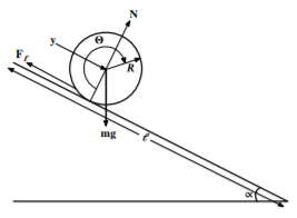
For example, for a disk rolling down an inclined plane without slipping, there are three coordinates $x$ [perpendicular to the wedge], $y$ , [Along the surface of the wedge], and the rotation angle $\theta$ shown in Figure 5.7.1. The constraint forces, $\mathbf{F}_{f}$ $\mathbf{N}$ , lead to the correlation of the variables such that $x=R$ , while $y=R\theta$ . Basically there is only one independent variable, which can be either $y$ or $\theta$ . The use of only one independent variable essentially buries the constraint forces under the rug, which is fine if you only need to know the equation of motion. If you need to determine the forces of constraint then it is necessary to include all coordinates explicitly in the equations of motion as discussed below.

Holonomic constraints¶

Most systems involve restrictions or constraints that couple the coordinates. For example, the $y_{i}(x)$ may be confined to a surface in coordinate space. The constraints mean that the coordinates $y_{i}(x)$ are not independent, but are related by equations of constraint. A constraint is called holonomic if the equations of constraint can be expressed in the form of an algebraic equation that directly and unambiguously specifies the shape of the surface of constraint. A non-holonomic constraint does not provide an algebraic relation between the correlated coordinates. In addition to the holonomy of the constraints, the equations of constraint also can be grouped into the following three classifications depending on whether they are algebraic, differential, or integral. These three classifications for the constraints exhibit different holonomy relating the coupled coordinates. Fortunately the solution of constrained systems is greatly simplified if the equations of constraint are holonomic.

Geometric (algebraic) equations of constraint¶

Geometric constraints can be expressed in the form of algebraic relations that directly specify the shape of the surface of constraint in coordinate space $q_{1},q_{2,}\dots ,q_{j},..q_{n}.$

g_{k}(q_{1},q_{2},..q_{j},..q_{n};t)=0 \tag{5.26}

where $j=1,2,3,\dots n$ . There can be $m$ such equations of constraint where $0\leq k\leq m$ . An example of such a geometric constraint is when the motion is confined to the surface of a sphere of radius $R$ in coordinate space which can be written in the form $g=x^{2}+y^{2}+z^{2}-R^{2}=0.$ Such algebraic constraint equations are called Holonomic which allows use of generalized coordinates as well as Lagrange multipliers to handle both the constraint forces and the correlation of the coordinates.

Kinematic (differential) equations of constraint¶

The $m$ constraint equations also can be expressed in terms of the infinitessimal displacements of the form

\sum_{j=1}^{n}\frac{\partial g_{k}}{\partial q_{j}}dq_{j}+\frac{\partial g_{k}}{\partial t}dt=0 \tag{5.27}

where $k=1,2,3,\dots m$ , $j=1,2,3,\dots n$ . If Equation 5.27 represents the total differential of a function then it can be integrated to give a holonomic relation of the form of Equation 5.26. However, if Equation 5.27 is not the total differential, then it is non-holonomic and can be integrated only after having solved the full problem.

An example of differential constraint equations is for a wheel rolling on a plane without slipping which is non-holonomic and more complicated than might be expected. The wheel moving on a plane has five degrees of freedom since the height $z$ is fixed. That is, the motion of the center of mass requires two coordinates $\left( x,y\right)$ plus there are three angles $(\phi ,\theta ,\psi )$ where $\phi$ is the rotation angle for the wheel, $\theta$ is the pivot angle of the axis, and $\psi$ is the tilt angle of the wheel. If the wheel slides then all five degrees of freedom are active. If the axis of rotation of the wheel is horizontal, that is, the tilt angle $\psi =0$ is constant, then this kinematic system leads to three differential constraint equations The wheel can roll with angular velocity $\dot{\phi}$ , as well as pivot which corresponds to a change in $\theta .$ Combining these leads to two differential equations of constraint

dx-a\sin \theta d\phi =0\hspace{1in}dy+a\cos \theta d\phi =0

These constraints are insufficient to provide finite relations between all the coordinates. That is, the constraints cannot be reduced by integration to the form of Equation 5.26 because there is no functional relation between $\phi$ and the other three variables, $x,y,\theta$ . Many rolling trajectories are possible between any two points of contact on the plane that are related to different pivot angles. That is, the point of contact of the disk could pivot plus roll in a circle returning to the same point where $x,y,\theta$ are unchanged whereas the value of $\phi$ depends on the circumference of the circle. As a consequence the rolling constraint is non-holonomic except for the case where the disk rolls in a straight line and remains vertical.

Isoperimetric (integral) equations of constraint¶

Equations of constraint also can be expressed in terms of direct integrals. This situation is encountered for isoperimetric problems, such as finding the maximum volume bounded by a surface of fixed area, or the shape of a hanging rope of fixed length. Integral constraints occur in economics when minimizing some cost algorithm subject to a fixed total cost constraint.

A simple example of an isoperimetric problem involves finding the curve $y=y(x)$ such that the functional has an extremum where the curve $y(x)$ satisfies boundary conditions such that $y(x_{1})=a$ and $y(x_{2})=b$ , that is

F(y)=\int_{x_{1}}^{x_{2}}f(y,y^{\prime };x)dx

is an extremum such that the perimeter also is constrained to satisfy

G(y)=\int_{x_{1}}^{x_{2}}g(y,y^{\prime };x)dx=l

where $l$ is a fixed length. This integral constraint is geometric and holonomic. Another example is finding the minimum surface area of a closed surface subject to the enclosed volume being the constraint.

Properties of the constraint equations¶

Holonomic constraints¶

Geometric constraints can be expressed in the form of an algebraic equation that directly specifies the shape of the surface of constraint

g(y_{1},y_{2},y_{3},\dots ;x)=0 \tag{5.31}

Such a system is called holonomic since there is a direct relation between the coupled variables. An example of such a holonomic geometric constraint is if the motion is confined to the surface of a sphere of radius $R$ which can be written in the form

g=x^{2}+y^{2}+z^{2}-R^{2}=0

Non-holonomic constraints¶

There are many classifications of non-holonomic constraints that exist if Equation 5.31 is not satisfied. The algebraic approach is difficult to handle when the constraint is an inequality, such as the requirement that the location is restricted to lie inside a spherical shell of radius $R$ which can be expressed as

g=x^{2}+y^{2}+z^{2}-R^{2}\leq 0

This non-holonomic constrained system has a one-sided constraint. Systems usually are non-holonomic if the constraint is kinematic as discussed above.

Partial Holonomic constraints¶

Partial-holonomic constraints are holonomic for a restricted range of the constraint surface in coordinate space, and this range can be case specific. This can occur if the constraint force is one-sided and perpendicular to the path. An example is the pendulum with the mass attached to the fulcrum by a flexible string that provides tension but not compression. Then the pendulum length is constant only if the tension in the string is positive. Thus the pendulum will be holonomic if the gravitational plus centrifugal forces are such that the tension in the string is positive, but the system becomes non-hononomic if the tension is negative as can happen when the pendulum rotates to an upright angle where the centrifugal force outwards is insufficient to compensate for the vertical downward component of the gravitational force. There are many other examples where the motion of an object is holonomic when the object is pressed against the constraint surface, such as the surface of the Earth, but is unconstrained if the object leaves the surface.

Time dependence¶

A constraint is called scleronomic if the constraint is not explicitly time dependent. This ignores the time dependence contained within the solution of the equations of motion. Fortunately a major fraction of systems are scleronomic. The constraint is called rheonomic if the constraint is explicitly time dependent. An example of a rheonomic system is where the size or shape of the surface of constraint is explicitly time dependent such as a deflating pneumatic tire.

Energy Conservation¶

The solution depends on whether the constraint is conservative or dissipative, that is, if friction or drag are acting. The system will be conservative if there are no drag forces, and the constraint forces are perpendicular to the trajectory of the path such as the motion of a charged particle in a magnetic field. Forces of constraint can result from sliding of two solid surfaces, rolling of solid objects, fluid flow in a liquid or gas, or result from electromagnetic forces. Energy dissipation can result from friction, drag in a fluid or gas, or finite resistance of electric conductors leading to dissipation of induced electric currents in a conductor, e.g. eddy currents.

A rolling constraint is unusual in that friction between the rolling bodies is necessary to maintain rolling. A disk on a frictionless inclined plane will conserve it’s angular momentum since there is no torque acting if the rolling contact is frictionless, that is, the disk will just slide. If the friction is sufficient to stop sliding, then the bodies will roll and not slide. A perfect rolling body does not dissipate energy since no work is done at the instantaneous point of contact where both bodies are in zero relative motion and the force is perpendicular to the motion. In real life, a rolling wheel can involve a very small energy dissipation due to deformation at the point of contact coupled with non-elastic properties of the material used to make the wheel and the plane surface. For example, a pneumatic tire can heat up and expand due to flexing of the tire.

Treatment of constraint forces in variational calculus¶

There are three major approaches to handle constraint forces in variational calculus. All three of them exploit the tremendous freedom and flexibility available when using generalized coordinates. The (1) generalized coordinate approach, described in chapter 5.8, exploits the correlation of the $n$ coordinates due to the $m$ constraint****forces to reduce the dimension of the equations of motion to $s=n-m$ degrees of freedom. This approach embeds the $m$ constraint forces, into the choice of generalized coordinates and does not determine the constraint forces, (2) Lagrange multiplier approach, described in chapter 5.9, exploits generalized coordinates but includes the $m$ constraint forces into the Euler equations to determine both the constraint forces in addition to the $n$ equations of motion. (3) Generalized forces approach, described in chapter $6.7.3,$ introduces constraint and other forces explicitly.

5.8: Generalized coordinates in Variational Calculus¶

Newtonian mechanics is based on a vectorial treatment of mechanics which can be difficult to apply when solving complicated problems in mechanics. Constraint forces acting on a system usually are unknown. In Newtonian mechanics constrained forces must be included explicitly so that they can be determined simultaneously with the solution of the dynamical equations of motion. The major advantage of the variational approaches is that solution of the dynamical equations of motion can be simplified by expressing the motion in terms of $n$ independent generalized coordinates. These generalized coordinates can be any set of independent variables, $q_{i}$ , where $1\leq i\leq n$ , plus the corresponding velocities $\dot{q}_{i}$ for Lagrangian mechanics, or the corresponding canonical variables, $q_{i},p_{i}$ for Hamiltonian mechanics. These generalized coordinates for the $n$ variables are used to specify the scalar functional dependence on these generalized coordinates. The variational approach employs this scalar functional to determine the trajectory. The generalized coordinates used for the variational approach do not need to be orthogonal, they only need to be independent since they are used only to completely specify the magnitude of the scalar functional. This greatly expands the arsenal of possible generalized coordinates beyond what is available using Newtonian mechanics. For example, generalized coordinates can be the dimensionless amplitudes for the $n$ normal modes of coupled oscillator systems, or action-angle variables. In addition, generalized coordinates having different dimensions can be used for each of the $n$ variables. Each generalized coordinate, $q_{i}$ specifies an independent mode of the system, not a specific particle. For example, each normal mode of coupled oscillators can involve correlated motion of several coupled particles. The major advantage of using generalized coordinates is that they can be chosen to be perpendicular to a corresponding constraint force, and therefore that specific constraint force does no work for motion along that generalized coordinate. Moreover, the constrained motion does no work in the direction of the constraint force for rigid constraints. Thus generalized coordinates allow specific constraint forces to be ignored in evaluation of the minimized functional. This freedom and flexibility of choice of generalized coordinates allows the correlated motion produced by the constraint forces to be embedded directly into the choice of the independent generalized coordinates, and the actual constraint forces can be ignored. Embedding of the constraint induced correlations into the generalized coordinates, effectively “sweeps the constraint forces under the rug” which greatly simplifies the equations of motion for any system that involve constraint forces. Selection of the appropriate generalized coordinates can be obvious, and often it is performed subconsciously by the user.

Three variational approaches are used that employ generalized coordinates to derive the equations of motion of a system that has $n$ generalized coordinates subject to $m$ constraints.

1) Minimal set of generalized coordinates: When the $m$ equations of constraint are holonomic, then the $m$ algebraic constraint relations can be used to transform the coordinates into $s=n-m$ independent generalized coordinates $q_{i}$ . This approach reduces the number of unknowns, $n,$ by the number of constraints $m$ , to give a minimal set of $s=n-m$ independent generalized dynamical variables. The forces of constraint are not explicitly discussed, or determined, when this generalized coordinate approach is employed. This approach greatly simplifies solution of dynamical problems by avoiding the need for explicit treatment of the constraint forces. This approach is straight forward for holonomic constraints, since the $n$ spatial coordinates $y_{1}(x),\dots y_{N}(x),$ are coupled by $m$ algebraic equations which can be used to make the transformation to generalized coordinates. Thus the $n$ coupled spatial coordinates are transformed to $s=n-m$ independent generalized dynamical coordinates $q_{1}(x),\dots .q_{s}(x)$ , and their generalized first derivatives $\dot{q}_{1}(x),\dots .\dot{q}_{s}(x).$ Thesegeneralized coordinates are independent, and thus it is possible to use Euler’s equation for each independent parameter $q_{i}$

\frac{\partial f}{\partial q_{i}}-\frac{d}{dx}\frac{\partial f}{\partial q_{i}^{\prime }}=0

where $i=1,2,3...s$ . There are $s=n-m$ such Euler equations. The freedom to choose generalized coordinates underlies the tremendous advantage of applying the variational approach.

2) Lagrange multipliers: The**** $n$ Lagrange equations, plus the $m$ equations of constraint, can be used to explicitly determine the $n$ generalized coordinates plus the $m$ constraint forces. That is, $n+m$ unknowns are determined. This approach is discussed in chapter 5.9.

3) Generalized forces: This approach introduces the constraint forces explicitly. This approach, applied to Lagrangian mechanics, is discussed in chapter 6.6.3.

The above three approaches exploit generalized coordinates to handle constraint forces as described in chapter 6.

5.9: Lagrange multipliers for Holonomic Constraints¶

Algebraic equations of constraint¶

The Lagrange multiplier technique provides a powerful, and elegant, way to handle holonomic constraints using Euler’s equations^[1]. The general method of Lagrange multipliers for $n$ variables, with $m$ constraints, is best introduced using Bernoulli’s ingenious exploitation of virtual infinitessimal displacements, which Lagrange signified by the symbol $\delta$ . The term “virtual” refers to an intentional variation of the generalized coordinates $\delta q_{i}$ in order to elucidate the local sensitivity of a function $F(q_{i},x)$ to variation of the variable. Contrary to the usual infinitessimal interval in differential calculus, where an actual displacement $dq_{i}$ occurs during a time $dt$ , a virtual displacement is imagined to be an instantaneous, infinitessimal, displacement of a coordinate, not an actual displacement, in order to elucidate the local dependence of $F$ on the coordinate. The local dependence of any functional $F,$ to virtual displacements of all $n$ coordinates, is given by taking the partial differentials of $F$ .

\delta F=\sum_{i}^{n}\frac{\partial F}{\partial q_{i}}\delta q_{i} \tag{5.35}

The function $F$ is stationary, that is an extremum, if Equation 5.35 equals zero. The extremum of the functional $F$ , given by equation (5.5.1), can be expressed in a compact form using the virtual displacement formalism as

\delta F=\delta \int_{x_{1}}^{x_{2}}\sum_{i}^{n}f\left[ q_{i}(x),q_{i}^{\prime }(x);x\right] dx=\sum_{i}^{n}\frac{\partial F}{\partial q_{i}}\delta q_{i}=0\tag{5.36}

The auxiliary conditions, due to the $m$ holonomic algebraic constraints for the $n$ variables $q_{i}$ , can be expressed by the $m$ equations

g_{k}(\mathbf{q})=0\tag{5.37}

where $1\leq k\leq m$ and $1\leq i\leq n$ with $m<n$ . The variational problem for the $m$ holonomic constraint equations also can be written in terms of $m$ differential equations where $1\leq k\leq m$

\delta g_{k}=\sum_{i=1}^{n}\frac{\partial g_{k}}{\partial q_{i}}\delta q_{i}=0\tag{5.38}

Since equations 5.36 and 5.38 both equal zero, the $m$ equations 5.38 can be multiplied by arbitrary undetermined factors $\lambda _{k},$ and added to equations 5.36 to give.

\delta F(q_{i},x)+\lambda _{1}\delta g_{1}+\lambda _{2}\delta g_{2}\cdot \cdot \lambda _{k}\delta g_{k}\cdot \cdot \lambda _{m}\delta g_{m}=0\tag{5.39}

Note that this is not trivial in that although the sum of the constraint equations for each $y_{i\text{ }}$ is zero; the individual terms of the sum are not zero.

Insert equations 5.36 plus 5.38 into 5.39, and collect all $n$ terms, gives

\sum_{i}^{n}\left( \frac{\partial F}{\partial q_{i}}+\sum_{k=1}^{m}\lambda _{k}\frac{\partial g_{k}}{\partial q_{i}}\right) \delta q_{i}=0\tag{5.40}

Note that all the $\delta q_{i}$ are free independent variations and thus the terms in the brackets, which are the coefficients of each $\delta q_{i}$ , individually must equal zero. For each of the $n$ values of $i$ , the corresponding bracket implies

\frac{\partial F}{\partial q_{i}}+\sum_{k=1}^{m}\lambda _{k}\frac{\partial g_{k}}{\partial q_{i}}=0\tag{5.41}

This is equivalent to what would be obtained from the variational principle

\delta F+\sum_{k=1}^{m}\lambda _{k}\delta g_{k}=0\tag{5.42}

Equation 5.42 is equivalent to a variational problem for finding the stationary value of $F^{\prime }$

\delta \left( F^{\prime }\right) =\delta \left( F+\sum_{k}^{m}\lambda _{k}g_{k}\right) =0\tag{5.43}

where $F^{\prime }$ is defined to be

F^{\prime }\equiv \left( F+\sum_{k=1}^{m}\lambda _{k}g_{k}\right)\tag{5.44}

The solution to Equation 5.43 can be found using Euler’s differential equation (5.5.4) of variational calculus. At the extremum $\delta \left( F^{\prime }\right) =0$ corresponds to following contours of constant $F^{\prime }$ which are in the surface that is perpendicular to the gradients of the terms in $F^{\prime }$ . The Lagrange multiplier constants are required because, although these gradients are parallel at the extremum, the magnitudes of the gradients are not equal.

The beauty of the Lagrange multipliers approach is that the auxiliary conditions do not have to be handled explicitly, since they are handled automatically as $m$ additional free variables during solution of Euler’s equations for a variational problem with $n+m$ unknowns fit to $n+m$ equations. That is, the $n$ variables $q_{i}$ are determined by the variational procedure using the $n$ variational equations

\frac{d}{dx}(\frac{\partial F^{\prime }}{\partial q_{i}^{\prime }})-(\frac{\partial F^{\prime }}{\partial q_{i}})=\frac{d}{dx}(\frac{\partial F}{\partial q_{i}^{\prime }})-(\frac{\partial F}{\partial q_{i}})-\sum_{k}^{m}\lambda _{k}\frac{\partial g_{k}}{\partial q_{i}}=0 \tag{5.45}

simultaneously with the $m$ variables $\lambda _{k}$ which are determined by the $m$ variational equations

\frac{d}{dx}(\frac{\partial F^{\prime }}{\partial \lambda _{k}^{\prime }})-(\frac{\partial F^{\prime }}{\partial \lambda _{k}})=0\tag{5.46}

Equation 5.45 usually is expressed as

(\frac{\partial F}{\partial q_{i}})-\frac{d}{dx}(\frac{\partial F}{\partial q_{i}^{\prime }})+\sum_{k}^{m}\lambda _{k}\frac{\partial g_{k}}{\partial q_{i}}=0 \tag{5.47}

The elegance of Lagrange multipliers is that a single variational approach allows simultaneous determination of all $n+m$ unknowns. Chapter 6.2 shows that the forces of constraint are given directly by the $\lambda _{k}\frac{\partial g_{k}}{\partial q_{i}}$ terms.

Example 5.9.1: Two dependent variables coupled by one holonomic constraint

The powerful, and generally applicable, Lagrange multiplier technique is illustrated by considering the case of only two dependent variables, $y(x),$ and $z\left( x\right) ,$ with the function $f(y(x),y^{\prime }(x),z(x),z(x)^{\prime };x)$ and with one holonomic equation of constraint coupling these two dependent variables. The extremum is given by requiring

\frac{\partial F}{\partial \epsilon }=\int_{x_{1}}^{x_{2}}\left[ \left( \frac{\partial f}{\partial y}-\frac{d}{dx}\frac{\partial f}{\partial y^{\prime }}\right) \frac{\partial y}{\partial \epsilon }+\left( \frac{\partial f}{\partial z}-\frac{d}{dx}\frac{\partial f}{\partial z^{\prime }}\right) \frac{\partial z}{\partial \epsilon }\right] dx=0 \tag{$A$}

with the constraint expressed by the auxiliary condition

g\left( y,z;x\right) =0 \tag{$B$}

Note that the variations $\frac{\partial y}{\partial \epsilon }$ and $\frac{\partial z}{\partial \epsilon }$ are no longer independent because of the constraint equation, thus the two terms in the brackets of Equation A are not separately equal to zero at the extremum. However, differentiating the constraint Equation B gives

\frac{dg}{d\epsilon }=\left( \frac{\partial g}{\partial y}\frac{\partial y}{\partial \epsilon }+\frac{\partial g}{\partial z}\frac{\partial z}{\partial \epsilon }\right) =0 \tag{$C$}

No $\frac{\partial g}{\partial x}$ term applies because, for the independent variable, $\frac{\partial x}{\partial \epsilon }$ $=0.$ Introduce the neighboring paths by adding the auxiliary functions

\begin{align} y(\epsilon ,x) &=&y(x)+\epsilon \eta _{1}(x) \tag{$D$} \\ z(\epsilon ,x) &=&z(x)+\epsilon \eta _{2}(x) \tag{$E$} \end{align}

Insert the differentials of equations D and E , into C gives

\frac{dg}{d\epsilon }=\left( \frac{\partial g}{\partial y}\eta _{1}(x)+\frac{\partial g}{\partial z}\eta _{2}(x)\right) =0 \tag{$F$}

implying that

\eta _{2}(x)=-\frac{\frac{\partial g}{\partial y}}{\frac{\partial g}{\partial z}}\eta _{1}(x) \nonumber

Equation A can be rewritten as

\begin{align} \int_{x_{1}}^{x_{2}}\left[ \left( \frac{\partial f}{\partial y}-\frac{d}{dx}\frac{\partial f}{\partial y^{\prime }}\right) \eta _{1}(x)+\left( \frac{\partial f}{\partial z}-\frac{d}{dx}\frac{\partial f}{\partial z^{\prime }}\right) \eta _{2}(x)\right] dx &=&0 \notag \\ \int_{x_{1}}^{x_{2}}\left[ \left( \frac{\partial f}{\partial y}-\frac{d}{dx}\frac{\partial f}{\partial y^{\prime }}\right) -\left( \frac{\partial f}{\partial z}-\frac{d}{dx}\frac{\partial f}{\partial z^{\prime }}\right) \frac{\frac{\partial g}{\partial y}}{\frac{\partial g}{\partial z}}\right] \eta _{1}(x)dx &=&0 \tag{$G$} \end{align}

Equation G now contains only a single arbitrary function $\eta _{1}(x)$ that is not restricted by the constraint. Thus the bracket in the integrand of Equation G must equal zero for the extremum. That is

\left( \frac{\partial f}{\partial y}-\frac{d}{dx}\frac{\partial f}{\partial y^{\prime }}\right) \left( \frac{\partial g}{\partial y}\right) ^{-1}=\left( \frac{\partial f}{\partial z}-\frac{d}{dx}\frac{\partial f}{\partial z^{\prime }}\right) \left( \frac{\partial g}{\partial z}\right) ^{-1}\equiv -\lambda (x) \notag

Now the left-hand side of this equation is only a function of $f$ and $g$ with respect to $y$ and $y^{\prime }$ while the right-hand side is a function of $f$ and $g$ with respect to $z$ and $z^{\prime }.$ Because both sides are functions of $x$ then each side can be set equal to a function $-\lambda (x).$ Thus the above equations can be written as

\frac{d}{dx}\frac{\partial f}{\partial y^{\prime }}-\frac{\partial f}{\partial y}=\lambda \left( x\right) \frac{\partial g}{\partial y}\hspace{1in}\frac{d}{dx}\frac{\partial f}{\partial z^{\prime }}-\frac{\partial f}{\partial z}=\lambda \left( x\right) \frac{\partial g}{\partial z} \tag{$H$}

The complete solution of the three unknown functions. $y(x),z(x),$ and $\lambda (x).$ is obtained by solving the two equations, H, plus the equation of constraint F. The Lagrange multiplier $\lambda (x)$ is related to the force of constraint. This example of two variables coupled by one holonomic constraint conforms with the general relation for many variables and constraints given by Equation 5.47.

Integral equations of constraint¶

The constraint equation also can be given in an integral form which is used frequently for isoperimetric problems . Consider a one dependent-variable isoperimetric problem, for finding the curve $q=q(x)$ such that the functional has an extremum, and the curve $q(x)$ satisfies boundary conditions such that $q(x_{1})=a$ and $q(x_{2})=b$ . That is

F(y)=\int_{x_{1}}^{x_{2}}f(q,q^{\prime };x)dx

is an extremum such that the fixed length $l$ of the perimeter satisfies the integral constraint

G(y)=\int_{x_{1}}^{x_{2}}g(q,q^{\prime };x)dx=l

Analogous to 5.44 these two functionals can be combined requiring that

\delta K(q,x,\lambda )\equiv \delta \left[ F(q)+\lambda G(q)\right] =\delta \int_{x_{1}}^{x_{2}}[f+\lambda g]dx=0

That is, it is an extremum for both $q(x)$ and the Lagrange multiplier $\lambda$ . This effectively involves finding the extremum path for the function $K(q,x,\lambda )=F(q,x)+\lambda G(q,x)$ where both $q(x)$ and $\lambda$ are the minimized variables. Therefore the curve $q(x)$ must satisfy the differential equation

\frac{d}{dx}\frac{\partial f}{\partial q_{i}^{\prime }}-\frac{\partial f}{\partial q_{i}}+\lambda \left[ \frac{d}{dx}\frac{\partial g}{\partial q_{i}^{\prime }}-\frac{\partial g}{\partial q_{i}}\right] =0 \tag{5.51}

subject to the boundary conditions $q(x_{1})=a,$ $q(x_{2})=b,$ and $G(q)=l$ .

Example 5.9.2: Catenary

One isoperimetric problem is the catenary which is the shape a uniform rope or chain of fixed length $l$ that minimizes the gravitational potential energy. Let the rope have a uniform mass per unit length of $\sigma$ kg/m.

Figure 5.9.1:The catenary

The gravitational potential energy is

U=\sigma g\int_{1}^{2}yds=\sigma g\int_{1}^{2}y\sqrt{dx^{2}+dy^{2}}=\sigma g\int_{1}^{2}y\sqrt{1+y^{\prime 2}}dx \notag

The constraint is that the length be a constant $l$

l=\int_{1}^{2}ds=\int_{1}^{2}\sqrt{1+y^{\prime 2}}dx \notag

Thus the function is $f(y,y^{\prime };x)=y\sqrt{1+y^{\prime 2}}$ while the integral constraint sets $g=\sqrt{1+y^{\prime 2}}$

These need to be inserted into the Euler Equation 5.51 by defining

F=f+\lambda g=(y+\lambda )\sqrt{1+y^{\prime 2}}\nonumber

Note that this case is one where $\frac{\partial F}{\partial x}=0$ and $\lambda$ is a constant; also defining $z=y+\lambda$ then $z^{\prime }=y^{\prime }.$ Therefore the Euler’s equations can be written in the integral form

F-z^{\prime }\frac{\partial F}{\partial z^{\prime }}=c=\text{constant}\nonumber

Inserting the relation $F=z\sqrt{1+z^{\prime 2}}$ gives

z\sqrt{1+z^{\prime 2}}-z^{\prime }\frac{zz^{\prime }}{\sqrt{1+z^{\prime 2}}}=c\nonumber

where $c$ is an arbitrary constant. This simplifies to

z^{\prime 2}=\left( \frac{z}{c}\right) ^{2}-1\nonumber

The integral of this is

z=c\cosh \left( \frac{x+b}{c}\right)\nonumber

where $b$ and $c$ are arbitrary constants fixed by the locations of the two fixed ends of the rope.

Example 5.9.3: The Queen Dido problem

A famous constrained isoperimetric legend is that of Dido, first Queen of Carthage. Legend says that, when Dido landed in North Africa, she persuaded the local chief to sell her as much land as an oxhide could contain. She cut an oxhide into narrow strips and joined them to make a continuous thread more than four kilometers in length which was sufficient to enclose the land adjoining the coast on which Carthage was built. Her problem was to enclose the maximum area for a given perimeter. Let us assume that the coast line is straight and the ends of the thread are at $\pm a$ on the coast line. The enclosed area is given by

A=\int_{-a}^{+a}ydx\nonumber

The constraint equation is that the total perimeter equals $l$ .

\int_{-a}^{a}\sqrt{1+y^{\prime 2}}dx=l\nonumber

Thus we have that the functional $f(y,y^{\prime },x)=y$ and $g(y,y^{\prime },x)=\sqrt{1+y^{\prime 2}}$ . Then $\frac{\partial f}{\partial y}=1,\frac{\partial f}{\partial y^{\prime }}=0,\frac{\partial g}{\partial y}=0$ and $\frac{\partial g}{\partial y^{\prime }}=\frac{y^{\prime }}{\sqrt{1+y^{\prime 2}}}.$ Insert these into the Euler-Lagrange Equation 5.51 gives

1-\lambda \frac{d}{dx}\left[ \frac{y^{\prime }}{\sqrt{1+y^{\prime 2}}}\right] =0\nonumber

That is

\frac{d}{dx}\left[ \frac{y^{\prime }}{\sqrt{1+y^{\prime 2}}}\right] =\frac{1}{\lambda }\nonumber

Integrate with respect to $x$ gives

\frac{\lambda y^{\prime }}{\sqrt{1+y^{\prime 2}}}=x-b\nonumber

where $b$ is a constant of integration. This can be rearranged to give

y^{\prime }=\frac{\pm \left( x-b\right) }{\sqrt{\lambda ^{2}-\left( x-b\right) ^{2}}}\nonumber

The integral of this is

y=\mp \sqrt{\lambda ^{2}-\left( x-b\right) ^{2}}+c\nonumber

Rearranging this gives

\left( x-b\right) ^{2}+\left( y-c\right) ^{2}=\lambda ^{2}\nonumber

This is the equation of a circle centered at $(b,c)$ . Setting the bounds to be $\left( -a,0\right)$ to $\left( a,0\right)$ gives that $b=c=0$ and the circle radius is $\lambda .$ Thus the length of the thread must be $l=\pi \lambda$ . Assuming that $l=4km$ then $\lambda =1.27km$ and Queen Dido could buy an area of $2.53km^{2}.$

5.10: Geodesic¶

The geodesic is defined as the shortest path between two fixed points for motion that is constrained to lie on a surface. Variational calculus provides a powerful approach for determining the equations of motion constrained to follow a geodesic.

The use of variational calculus is illustrated by considering the geodesic constrained to follow the surface of a sphere of radius $R$ . As discussed in appendix $19.3.2C$ , the element of path length on the surface of the sphere is given in spherical coordinates as $ds=R \sqrt{d\theta ^{2}+\left( \sin \theta d\phi \right) ^{2}}$ . Therefore the distance $s$ between two points 1 and 2 is

s=R\int_{1}^{2}\left[ \sqrt{\left( \frac{d\theta }{d\phi }\right) ^{2}+\sin ^{2}\theta }\right] d\phi

The function $f$ for ensuring that $s$ be an extremum value uses

f=\sqrt{\theta ^{\prime 2}+\sin ^{2}\theta }

where $\theta ^{\prime }=\frac{d\theta }{d\phi }.$ This is a case where $\frac{\partial f}{\partial \phi }=0$ and thus the integral form of Euler’s equation can be used leading to the result that

\sqrt{\theta ^{\prime 2}+\sin ^{2}\theta }-\theta ^{\prime }\frac{\partial }{ \partial \theta ^{\prime }}\sqrt{\theta ^{\prime 2}+\sin ^{2}\theta }=\text{ constant}=a

This gives that

\sin ^{2}\theta =a\sqrt{\theta ^{\prime 2}+\sin ^{2}\theta }

This can be rewritten as

\frac{d\phi }{d\theta }=\frac{1}{\theta ^{\prime }}=\frac{a\csc ^{2}\theta }{ \sqrt{1-a^{2}\csc ^{2}\theta }}

Solving for $\phi$ gives

\phi =\sin ^{-1}\left( \frac{\cot \theta }{\beta }\right) +\alpha

where

\beta \equiv \frac{1-a^{2}}{a^{2}}

That is

\cot \theta =\beta \sin \left( \phi -\alpha \right)

Expanding the sine and cotangent gives

\left( \beta \cos \alpha \right) R\sin \theta \sin \phi -\left( \beta \sin \alpha \right) R\sin \theta \cos \phi =R\cos \theta

Since the brackets are constants, this can be written as

A\left( R\sin \theta \sin \phi \right) -B\left( R\sin \theta \cos \phi \right) =\left( R\cos \theta \right)

The terms in the brackets are just expressions for the rectangular coordinates $x,y,z.$ That is,

Ay-Bx=z

This is the equation of a plane passing through the center of the sphere. Thus the geodesic on a sphere is the path where a plane through the center intersects the sphere as well as the initial and final locations. This geodesic is called a great circle. Euler’s equation gives both the maximum and minimum extremum path lengths for motion on this great circle.

Chapter 17 discusses the geodesic in the four-dimensional space-time coordinates that underlie the General Theory of Relativity. As a consequence, the use of the calculus of variations to determine the equations of motion for geodesics plays a pivotal role in the General Theory of Relativity.

5.11: Variational Approach to Classical Mechanics¶

This chapter has introduced the general principles of variational calculus needed for understanding the Lagrangian and Hamiltonian approaches to classical mechanics. Although variational calculus was developed originally for classical mechanics, now it has grown to be an important branch of mathematics with applications to many other fields outside of physics. The prologue of this book emphasized the dramatic differences between the differential vectorial approach of Newtonian mechanics, and the integral variational approaches of Lagrange and Hamiltonian mechanics. The Newtonian vectorial approach involves solving Newton’s differential equations of motion that relate the force and momenta vectors. This requires knowledge of the time dependence of all the force vectors, including constraint forces, acting on the system which can be very complicated. Chapter 2 showed that the first-order time integrals, equations (2.4.1), (2.4.7), relate the initial and final total momenta without requiring knowledge of the complicated instantaneous forces acting during the collision of two bodies. Similarly, for conservative systems, the first-order spatial integral, equation (2.4.12), relates the initial and final total energies to the net work done on the system without requiring knowledge of the instantaneous force vectors. The first-order spatial integral has the advantage that it is a scalar quantity, in contrast to time integrals which are vector quantities. These first-order integral relations are used frequently in Newtonian mechanics to derive solutions of the equations of motion that avoid having to solve complicated differential equations of motion.

This chapter has illustrated that variational principles provide a means of deriving more detailed information, such as the trajectories for the motion between given initial and final conditions, by requiring that scalar functionals have extrema values. For example, the solution of the brachistochrone problem determined the trajectory having the minimum transit time, based on only the magnitudes of the kinetic and gravitational potential energies. Similarly, the catenary shape of a suspended chain was derived by minimizing the gravitational potential energy. The calculus of variations uses Euler’s equations to determine directly the differential equations of motion of the system that lead to the functional of interest being stationary at an extremum. The Lagrangian and Hamiltonian variational approaches to classical mechanics are discussed in chapters $6-16$ . The broad range of applicability, the flexibility, and the power provided by variational approaches to classical mechanics and modern physics will be illustrated.

5.E: Calculus of Variations (Exercises)¶

Find the extremal of the functional

J(x) = \int^2_1 \frac{\dot{x}^2}{t^3} dt \nonumber

that satisfies $x(1) = 3$ and $x(2) = 18$ . Show that this extremal provides the global minimum of $J$ .

Consider the use of equations of constraint.
A particle is constrained to move on the surface of a sphere. What are the equations of constraint for this system?
A disk of mass $m$ and radius $R$ rolls without slipping on the outside surface of a half-cylinder of radius $5R$ . What are the equations of constraint for this system?
What are holonomic constraints? Which of the equations of constraint that you found above are holonomic?
Equations of constraint that do not explicitly contain time are said to be scleronomic. Moving constraints are rheonomic. Are the equations of constraint that you found above scleronomic or rheonomic?
For each of the following systems, describe the generalized coordinates that would work best. There may be more than one answer for each system.
An inclined plane of mass $M$ is sliding on a smooth horizontal surface, while a particle of mass $m$ is sliding on the smooth inclined surface.
A disk rolls without slipping across a horizontal plane. The plane of the disk remains vertical, but it is free to rotate about a vertical axis.
A double pendulum consisting of two simple pendula, with one pendulum suspended from the bob of the other. The two pendula have equal lengths and have bobs of equal mass. Both pendula are confined to move in the same plane.
A particle of mass $m$ is constrained to move on a circle of radius $R$ . The circle rotates in space about one point on the circle, which is fixed. The rotation takes place in the plane of the circle, with constant angular speed $\omega$ , in the absence of a gravitational force.
A particle of mass $m$ is attracted toward a given point by a force of magnitude $k/r^2$ , where $k$ is a constant.
Looking back at the systems in problem 3, which ones could have equations of constraint? How would you classify the equations of constraint (holonomic, scleronomic, rheonomic, etc.)?
Find the extremal of the functional
$J(x) = \int^{\pi}_0 (2x \sin t - \dot{x}^2) dt\nonumber$
that satisfies $x(o) = x(\pi) = 0$ . Show that this extremal provides the global maximum of $J$ .
Find and describe the path $y = y(x)$ for which the integral $\int^{x_2}_{x_1} \sqrt{x} \sqrt{1 + (y^{\prime})^2} dx$ is stationary.
Find the dimensions of the parallelepiped of maximum volume circumscribed by a sphere of radius $R$ .
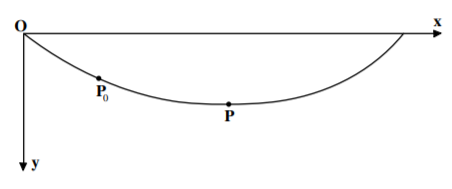
Consider a single loop of the cycloid having a fixed value of $a$ as shown in the figure. A car released from rest at any point $P_0$ anywhere on the track between $O$ and the lowest point $P$ , that is, $P_0$ has a parameter $0 < \theta_0 < \pi$ .

Show that the time $T$ for the cart to slide from $P_0$ to $P$ is given by the integral
$T(P_0 \rightarrow P) = \sqrt{\frac{a}{g}} \int^{\pi}_{\theta_0} \sqrt{\frac{1 − \cos \theta}{ \cos \theta_0 − \cos \theta}} d\theta\nonumber$
Prove that this time $T$ is equal to $\pi \sqrt{a/g}$ which is independent of the position $P_0$ .
Explain qualitatively how this surprising result can possibly be true.
Consider a medium for which the refractive index $n = \frac{a}{r^2}$ where $a$ is a constant and $r$ is the distance from the origin. Use Fermat’s Principle to find the path of a ray of light travelling in a plane containing the origin. Hint, use two-dimensional polar coordinates with $\phi = \phi (r)$ . Show that the resulting path is a circle through the origin.
Find the shortest path between the $(x, y, z)$ points $(0, −1, 0)$ and $(0, 1, 0)$ on a conical surface
$z = 1 − \sqrt{x^2 + y^2}\nonumber$
What is the length of this path? Note that this is the shortest mountain path around a volcano.
Show that the geodesic on the surface of a right circular cylinder is a segment of a helix.

5.S: Calculus of Variations (Summary)¶

Euler’s differential equation¶

The calculus of variations has been introduced and Euler’s differential equation was derived. The calculus of variations reduces to varying the functions $y_{i}(x),$ where $i=1,2,3,...n$ , such that the integral

F=\int_{x_{1}}^{x_{2}}f\left[ y_{i}(x),y_{i}^{\prime }(x);x\right] dx

is an extremum, that is, it is a maximum or minimum. Here $x$ is the independent variable, $y_{i}(x)$ are the dependent variables plus their first derivatives $y_{i}^{\prime }\equiv \frac{dy_{i}}{dx}.$ The quantity $f\left[ y(x),y^{\prime }(x);x\right]$ has some given dependence on $y_{i},y_{i}^{\prime }$ and $\ x.$ The calculus of variations involves varying the functions $y_{i}(x)$ until a stationary value of $F$ is found which is presumed to be an extremum. It was shown that if the $y_{i}(x)$ are independent, then the extremum value of $F$ leads to $n$ independent Euler equations

\frac{\partial f}{\partial y_{i}}-\frac{d}{dx}\frac{\partial f}{\partial y_{i}^{\prime }}=0

where $i=1,2,3..n$ . This can be used to determine the functional form $y_{i}(x)$ that ensures that the integral $F=\int_{x_{1}}^{x_{2}}f\left[ y(x),y^{\prime }(x);x\right] dx$ is a stationary value, that is, presumably a maximum or minimum value.

Note that Euler’s equation involves partial derivatives for the dependent variables $y_{i},y_{i}^{\prime },$ and the total derivative for the independent variable $x.$

Euler’s integral equation¶

It was shown that if the function $\int_{x_{1}}^{x_{2}}f\left[ y_{i}(x),y_{i}^{\prime }(x);x\right]$ does not depend on the independent variable, then Euler’s differential equation can be written in an integral form. This integral form of Euler’s equation is especially useful when $\frac{\partial f}{\partial x}=0,$ that is, when $f$ does not depend explicitly on $x$ , then the first integral of the Euler equation is a constant

f-y^{\prime }\frac{\partial f}{\partial y^{\prime }}=\text{constant}

Constrained variational systems¶

Most applications involve constraints on the motion. The equations of constraint can be classified according to whether the constraints are holonomic or non-holonomic, the time dependence of the constraints, and whether the constraint forces are conservative.

Generalized coordinates in variational calculus¶

Independent generalized coordinates can be chosen that are perpendicular to the rigid constraint forces and therefore the constraint does not contribute to the functional being minimized. That is, the constraints are embedded into the generalized coordinates and thus the constraints can be ignored when deriving the variational solution.

Minimal set of generalized coordinates¶

If the constraints are holonomic then the $m$ holonomic equations of constraint can be used to transform the $n$ coupled generalized coordinates to $s=n-m$ independent generalized variables $q_{i},q_{i}^{\prime }$ . The generalized coordinate method then uses Euler’s equations to determine these $s=n-m$ independent generalized coordinates.

\frac{\partial f}{\partial q_{i}}-\frac{d}{dx}\frac{\partial f}{\partial q_{i}^{\prime }}=0

Lagrange multipliers for holonomic constraints¶

The Lagrange multipliers approach for $n$ variables, plus $m$ holonomic equations of constraint, determines all $N + m$ unknowns for the system. The holonomic forces of constraint acting on the $N$ variables, are related to the Lagrange multiplier terms $\lambda_k(x)\frac{\partial g_k}{\partial y_i})$ that are introduced into the Euler equations.

That is,

\frac{\partial f}{\partial y_i}- \frac{d f}{d x} \frac{\partial f}{\partial y^\prime_i} + \sum_k^m\lambda_k(x)\frac{\partial g_k}{\partial y_i}

where the holonomic equations of constraint are given by

g_k(y_i;x)=0

The advantage of using the Lagrange multiplier approach is that the variational procedure simultaneously determines both the equations of motion for the $N$ variables plus the $m$ constraint forces acting on the system.

Footnotes¶

This textbook uses the symbol $q_i$ to designate a generalized coordinate, and $q^{\prime}_i$ to designate the corresponding first derivative with respect to the independent variable, in order to differentiate the spatial coordinates from the more powerful generalized coordinates.
↩

5.1: Introduction to the Calculus of Variations¶

5.2: Euler’s Differential Equation¶

5.3: Applications of Euler’s Equation¶

5.4: Selection of the Independent Variable¶

5.5: Functions with Several Independent Variables¶

Functions with several independent variables yi(x)y_{i}(x)yi​(x)¶

5.6: Euler’s Integral Equation¶

5.7: Constrained Variational Systems¶

Holonomic constraints¶

Geometric (algebraic) equations of constraint¶

Kinematic (differential) equations of constraint¶

Isoperimetric (integral) equations of constraint¶

Properties of the constraint equations¶

Holonomic constraints¶

Non-holonomic constraints¶

Partial Holonomic constraints¶

Time dependence¶

Energy Conservation¶

Treatment of constraint forces in variational calculus¶

5.8: Generalized coordinates in Variational Calculus¶

5.9: Lagrange multipliers for Holonomic Constraints¶

Algebraic equations of constraint¶

Integral equations of constraint¶

5.10: Geodesic¶

5.11: Variational Approach to Classical Mechanics¶

5.E: Calculus of Variations (Exercises)¶

5.S: Calculus of Variations (Summary)¶

Euler’s differential equation¶

Euler’s integral equation¶

Constrained variational systems¶

Generalized coordinates in variational calculus¶

Minimal set of generalized coordinates¶

Lagrange multipliers for holonomic constraints¶

Functions with several independent variables $y_{i}(x)$ ¶