17.1: Introduction to Relativistic Mechanics
Newtonian mechanics incorporates the Newtonian concept of the complete separation of space and time. This theory reigned supreme from inception, in 1687, until November 1905 when Einstein pioneered the Special Theory of Relativity. Relativistic mechanics undermines the Newtonian concepts of absoluteness of time that is inherent to Newton’s formulation, as well as when recast in the Lagrangian and Hamiltonian formulations of classical mechanics. Relativistic mechanics has had a profound impact on twentieth-century physics and the philosophy of science. Classical mechanics is an approximation of relativistic mechanics that is valid for velocities much less than the velocity of light in vacuum. The term “relativity” refers to the fact that physical measurements are always made relative to some chosen reference frame. Naively one may think that the transformation between different reference frames is trivial and contains little underlying physics. However, Einstein showed that the results of measurements depend on the choice of coordinate system, which revolutionized our concept of space and time.
Einstein’s work on relativistic mechanics comprised two major advances. The first advance is the 1905 Special Theory of Relativitywhich refers to nonaccelerating frames of reference. The second major advance was the 1916 General Theory of Relativity which considers accelerating frames of reference and their relation to gravity. The Special Theory is a limiting case of the General Theory of Relativity. The mathematically complex General Theory of Relativity is required for describing accelerating frames, gravity, plus related topics like Black Holes, or extremely accurate time measurements inherent to the Global Positioning System. The present discussion will focus primarily on the mathematically simple Special Theory of Relativity since it encompasses most of the physics encountered in atomic, nuclear and high energy physics. This chapter uses the basic concepts of the Special Theory of Relativity to investigate the implications of extending Newtonian, Lagrangian and Hamiltonian formulations of classical mechanics into the relativistic domain. The Lorentz-invariant extended Hamiltonian and Lagrangian formalisms are introduced since they are applicable to the Special Theory of Relativity. The General Theory of Relativity incorporates the gravitational force as a geodesic phenomena in a four-dimensional Riemannian structure based on space, time, and matter. A superficial outline is given to the fundamental concepts and evidence that underlie the General Theory of Relativity.
17.2: Galilean Invariance
As discussed in chapter 2.3, an inertial frame is one in which Newton’s Laws of motion apply. Inertial frames are non-accelerating frames so that pseudo forces are not induced. All reference frames moving at constant velocity relative to an inertial reference, are inertial frames. Newton’s Laws of nature are the same in all inertial frames of reference and therefore there is no way of determining absolute motion because no inertial frame is preferred over any other. This is called Galilean-Newtonian invariance. Galilean invariance assumes that the concepts of space and time are completely separable. Time is assumed to be an absolute quantity that is invariant to transformations between coordinate systems in relative motion. Also the element of length is the same in different Galilean frames of reference.
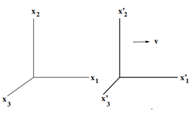
Figure 17.2.1:Motion of the primed frame along the axis with velocity relative to the parallel unprimed frame.
Consider two coordinate systems shown in Figure 17.2.1, where the primed frame is moving along the axis of the fixed unprimed frame. A Galilean transformation implies that the following relations apply;
Note that at any instant , the infinitesimal units of length in the two systems are identical since
These are the mathematical expression of the Newtonian idea of space and time. An immediate consequence of the Galilean transformation is that the velocity of light must differ in different inertial reference frames.
At the end of the 19 century physicists thought they had discovered a way of identifying an absolute inertial frame of reference, that is, it must be the frame of the medium that transmits light in vacuum. Maxwell’s laws of electromagnetism predict that electromagnetic radiation in vacuum travels at . Maxwell did not address in what frame of reference that this speed applied. In the nineteenth century all wave phenomena were transmitted by some medium, such as waves on a string, water waves, sound waves in air. Physicists thus envisioned that light was transmitted by some unobserved medium which they called the ether. This ether had mystical properties, it existed everywhere, even in outer space, and yet had no other observed consequences. The ether obviously should be the absolute frame of reference.
In the 1880’s, Michelson and Morley performed an experiment in Cleveland to try to detect this ether. They transmitted light back and forth along two perpendicular paths in an interferometer, shown in Figure 17.2.2, and assumed that the earth’s motion about the sun led to movement through the ether.
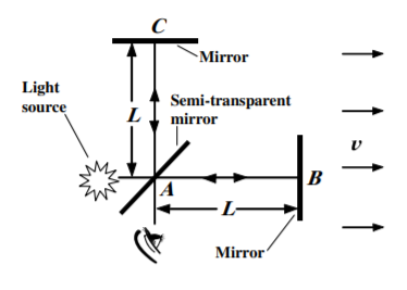
Figure 17.2.2:The Michelson interferometer used for the Michelson-Morley experiment. Interference of the two beams of coherent light leads to fringes that depends on the differences in phase along the two paths.
The time taken to travel a return trip takes longer in a moving medium, if the medium moves in the direction of the motion, compared to travel in a stationary medium. For example, you lose more time moving against a headwind than you gain traveling back with the wind. The time difference , for a round trip to a distance , between traveling in the direction of motion in the ether, versus traveling the same distance perpendicular to the movement in the ether, is given by where is the relative velocity of the ether and is the velocity of light.
Interference fringes between perpendicular light beams in an optical interferometer provides an extremely sensitive measure of this time difference. Michelson and Morley observed no measurable time difference at any time during the year, that is, the relative motion of the earth within the ether is less than the velocity of the earth around the sun. Their conclusion was either, that the ether was dragged along with the earth, or the velocity of light was dependent on the velocity of the source, but these did not jibe with other observations. Their disappointment at the failure of this experiment to detect evidence for an absolute inertial frame is important and confounded physicists for two decades until Einstein’s Special Theory of Relativity explained the result.
17.3: Special Theory of Relativity
Einstein Postulates
In November 1905, at the age of 26, Einstein published a seminal paper entitled ”On the electrodynamics of moving bodies”. He considered the relation between space and time in inertial frames of reference that are in relative motion. In this paper he made the following postulates.
The laws of nature are the same in all inertial frames of reference.
The velocity of light in vacuum is the same in all inertial frames of reference.
Note that Einstein’s first postulate, coupled with Maxwell’s equations, leads to the statement that the velocity of light in vacuum is a universal constant. Thus the second postulate is unnecessary since it is an obvious consequence of the first postulate plus Maxwell’s equations which are basic laws of physics. This second postulate explained the null result of the Michelson-Morley experiment. However, it was not this experimental result that led Einstein to the theory of special relativity; he deduced the Special Theory of Relativity from consideration of Maxwell’s equations of electromagnetism. Although Einstein’s postulates appear reasonable, they lead to the following surprising implications.
Lorentz transformation
Galilean invariance leads to violation of the Einstein postulate that the velocity of light is a universal constant in all frames of reference. It is necessary to assume a new transformation law that renders physical laws relativistically invariant. Maxwell’s equations are relativistically invariant, which led to some electromagnetic phenomena that could not be explained using Galilean invariance. In 1904 Lorentz proposed a new transformation to replace the Galilean transformation in order to explain such electromagnetic phenomena. Einstein’s genius was that he derived the transformation, that had been proposed by Lorentz, directly from the postulates of the Special Theory of Relativity. The Lorentz transformation satisfies Einstein’s theory of relativity, and has been confirmed to be correct by many experiments.
For the geometry shown in Figure 17.2.1, the Lorentz transformations are:
where the Lorentz factor
The inverse transformations are
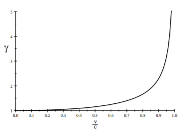
Figure 17.3.1:The dependence of the Lorentz factor on .
The Lorentz factor, defined above, is the key feature differentiating the Lorentz transformations from the Galilean transformation. Note that ; also as and increases to infinity as as illustrated in Figure 17.3.1. A useful fact that will be used later is that for ;
Note that for then and the Lorentz transformation is identical to the Galilean transformation.
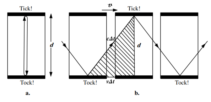
Figure 17.3.2:The observer and mirror are at rest in the left-hand frame (a). The light beam takes a time to travel to the mirror. In the right-hand frame (b) the source and mirror are traveling at a velocity relative to the observer. The light travels further in the right-hand frame of reference (b) than is the stationary frame (a). Since Einstein states that the velocity of light is the same in both frames of reference then the time interval must by larger in frame (b) since the light travels further than in (a).
Time Dilation
Consider that a clock is fixed at in a moving frame and measures the time interval between two events in the moving frame, i.e. . According to the Lorentz transformation, the times in the fixed frame are given by:
Thus the time interval is given by:
The time between events in the rest frame of the clock, is called the proper time which always is the shortest time measured for a given event and is represented by the symbol . That is
Note that the time interval for any other frame of reference, moving with respect to the clock frame, will show larger time intervals because which implies that the fixed frame perceives that the moving clock is slow by the factor .
The plausibility of this time dilation can be understood by looking at the simple geometry of the space ship example shown in Figure 17.3.2. Pretend that the clock in the proper frame of the space ship is based on the time for the light to travel to and from the mirror in the space ship. In this proper frame the light has the shortest distance to travel, and the proper transit time is
In the fixed frame, , the component of velocity in the direction of the mirror is using the Pythagorean theorem, assuming that the light cannot travel faster than . Thus the transit time towards and back from the mirror must be
which is the predicted time dilation.
There are many experimental verifications of time dilation in physics. For example, a stationary muon has a mean lifetime of , whereas the lifetime of a fast moving muon, produced in the upper atmosphere by high-energy cosmic rays, was observed in 1941 to be longer and given by as described in example 17.3.1. In 1972 Hafele and Keating used four accurate cesium atomic clocks to confirm time dilation. Two clocks were flown on regularly scheduled airlines traveling around the World, one westward and the other eastward. The other two clocks were used for reference. The westward moving clock was slow by compared to the predicted value of . The Global Positioning System of 24 geosynchronous satellites is used for locating positions to within a few meters. It has an accuracy of a few nanoseconds which requires allowance for time dilation and is a daily tribute to the correctness of Einstein’s Theory of Relativity.
Length Contraction
The Lorentz transformation leads to a contraction of the apparent length of an object in a moving frame as seen from a fixed frame. The length of a ruler in its own frame of reference is called the proper length. Consider an accurately measured rod of known proper length that is, at rest in the moving primed frame. The locations of both ends of this rod are measured at a given time in the stationary frame, , by taking a photograph of the moving rod. The corresponding locations in the moving frame are:
Since , the measured lengths in the two frames are related by:
That is, the lengths are related by:
Note that the moving rod appears shorter in the direction of motion. As the apparent length shrinks to zero in the direction of motion while the dimensions perpendicular to the direction of motion are unchanged. This is called the Lorentz contraction. If you could ride your bicycle at close to the speed of light, you would observe that stationary cars, buildings, people, all would appear to be squeezed thin along the direction that you are traveling. Also objects that are further away down any side street would be distorted in the direction of travel. A photograph taken by a stationary observer would show the moving bicycle to be Lorentz contracted along the direction of travel and the stationary objects would be normal.
Simultaneity
The Lorentz transformations imply a new philosophy of space and time. A surprising consequence is that the concept of simultaneity is frame dependent in contrast to the prediction of Newtonian mechanics.
Consider that two events occur in frame at and . In frame these two events occur at and . From the Lorentz transformation the time difference is
If an event is simultaneous in frame , that is then
Thus the event is not simultaneous in frame if . That is, an event that is simultaneous in one frame is not simultaneous in the other frame if the events are spatially separated. The equivalent statement is that for two clocks, spatially separated by a distance , which are synchronized in their rest frame, then in a moving frame they are not simultaneous.
Einstein discussed the problem of lightning striking both ends of a railway carriage that is moving at a velocity . Assume that the lightning strikes both the front and rear of the carriage simultaneously, according to a stationary observer. A woman riding in the center of the train will se the lightning flash arrive from the front of the carriage before the wavefront from the rear of the carriage arrives since the carriage is moving towards the approaching wavefront and away from the wavefront from the rear of the train. If the length of the carriage is , then the time difference between the light flash from front and rear of the carriage will be . As a consequence she observes that the two signals are not simultaneous. Thus a photograph of a rapidly moving body will appear to have a shorter distance. The relativistic snake discussed in chapter 17, exercise 1 is a similar example of the role of simultaneity in relativistic mechanics.
17.4: Relativistic Kinematics
Velocity Transformations
Consider the two parallel coordinate frames with the primed frame moving at a velocity along the axis as shown in Figure 17.2.1. Velocities of an object measured in both frames are defined to be
Using the Lorentz transformations , between the two frames moving with relative velocity along the axis, gives that the velocity along the axis is
Similarly we get the velocities along the perpendicular and axes to be
When these velocity transformations become the usual Galilean relations for velocity addition. Do not confuse and with ; that is, and are the velocities of some object measured in the unprimed and primed frames of reference respectively, whereas is the relative velocity of the origin of one frame with respect to the origin of the other frame.
Momentum
Using the classical definition of momentum, that is , the linear momentum is not conserved using the above relativistic velocity transformations if the mass is a scalar quantity. This problem originates from the fact that both and have non-trivial transformations and thus is frame dependent.
Linear momentum conservation can be retained by redefining momentum in a form that is identical in all frames of reference, that is by referring to the proper time as measured in the rest frame of the moving object. Therefore we define relativistic linear momentum as
But we know the time dilation relation
Note that the in this relation refers to the velocity between the moving object and the frame; this is quite different from the which refers to the transformation between the two frames of reference. Thus the new relativistic definition of momentum is
The relativistic definition of linear momentum is the same as the classical definition with the rest mass replaced by the relativistic mass .[1]
Center of momentum coordinate system
The classical relations for handling the kinematics of colliding objects, carry over to special relativity when the relativistic definition of linear momentum, Equation 17.21, is assumed. That is, one can continue to apply conservation of linear momentum. However, there is one important conceptual difference for relativistic dynamics in that the center of mass no longer is a meaningful concept due to the interrelation of mass and energy. However, this problem is eliminated by considering the center of momentum coordinate system which, as in the non-relativistic case, is the frame where the total linear momentum of the system is zero. Using the concept of center of momentum incorporates the formalism of classical non-relativistic kinematics.
Force
Newton’s second law is covariant under a Galilean transformation. In special relativity this definition also applies using the relativistic definition of momentum . The fact that the relativistic momentum is conserved in the force-free situation, leads naturally to using the definition of force to be
Then the relativistic momentum is conserved if .
Energy
The classical definition of work done is defined by
Assume , let and insert the relativistic force relation in Equation 17.23, gives
Integrate by parts, followed by algebraic manipulation, gives
Define the rest energy
and total relativistic energy
then Equation 17.25 can be written as
This is the famous Einstein relativistic energy that relates the equivalence of mass and energy. The total relativistic energy is a conserved quantity in nature. It is an extension of the conservation of energy and manifestations of the equivalence of energy and mass occur extensively in the real world.
In nuclear physics we often convert mass to energy and back again to mass. For example, gamma rays with energies greater than 1.022 , which are pure electromagnetic energy, can be converted to an electron plus positron both of which have rest mass. The positron can then annihilate a different electron in another atom resulting in emission of two 511 gamma rays in back to back directions to conserve linear momentum. A dramatic example of Einstein’s equation is a nuclear reactor. One gram of material, the mass of a paper clip, provides joules. This is the daily output of a 1 nuclear power station or the explosive power of the Nagasaki or Hiroshima bombs.
As the velocity of a particle approaches , then and the relativistic mass both approach infinity. This means that the force needed to accelerate the mass also approaches infinity, and thus no particle can exceed the velocity of light. The energy continues to increase not by increasing the velocity but by increase of the relativistic mass. Although the relativistic relation for kinetic energy is quite different from the Newtonian relation, the Newtonian form is obtained for the case of in that
An especially useful relativistic relation that can be derived from the above is
This is useful because it provides a simple relation between total energy of a particle and its relativistic linear momentum plus rest energy.
17.5: Geometry of Space-time
Four-Dimensional Space-Time
In 1906 Poincaré showed that the Lorentz transformation can be regarded as a rotation in a 4-dimensional Euclidean space-time introduced by adding an imaginary fourth space-time coordinate to the three real spatial coordinates. In 1908 Minkowski reformulated Einstein’s Special Theory of Relativity in this 4-dimensional Euclidean space-time vector space and concluded that the spatial variables , where , plus the time are equivalent variables and should be treated equally using a covariant representation of both space and time. The idea of using an imaginary time axis to make space-time Euclidean was elegant, but it obscured the non-Euclidean nature of space-time as well as causing difficulties when generalized to non-inertial accelerating frames in the General Theory of Relativity. As a consequence, the use of the imaginary has been abandoned in modern work. Minkowski developed an alternative non-Euclidean metric that treats all four coordinates as a four-dimensional Minkowski metric with all coordinates being real, and introduces the required minus sign explicitly.
Analogous to the usual 3-dimensional cartesian coordinates, the displacement four vector is defined using the four components along the four unit vectors in either the unprimed or primed coordinate frames.
The convention used is that greek subscripts (covariant) or superscripts (contravariant) designate a four vector with . The covariant unit vectors are written with the subscript which has 4 values . As described in appendix 19.5.3, using the Einstein convention the components are written with the contravariant superscript where the time axis , while the spatial coordinates, expressed in cartesian coordinates, are , , and . With respect to a different (primed) unit vector basis , the displacement must be unchanged as given by Equation 17.31. In addition, Equation 17.43 shows that the magnitude of the displacement four vector is invariant to a Lorentz transformation.
The most general Lorentz transformation between inertial coordinate systems and , in relative motion with velocity , assuming that the two sets of axes are aligned, and that their origins overlap when , is given by the symmetric matrix where
This Lorentz transformation of the four vector components can be written in matrix form as
Assuming that the two sets of axes are aligned, then the elements of the Lorentz transformation are given by
where and and assuming that the origin of transforms to the origin of at .
For the case illustrated in Figure 17.2.1, where the corresponding axes of the two frames are parallel and in relative motion with velocity in the direction, then the Lorentz transformation matrix 17.34 reduces to
This Lorentz transformation matrix is called a standard boost since it only boosts from one frame to another parallel frame. In general a rotation matrix also is incorporated into the transformation matrix for the spatial variables.
Four-vector scalar products
Scalar products of vectors and tensors usually are invariant to rotations in three-dimensional space providing an easy way to solve problems. The scalar, or inner, product of two four vectors is defined by
The correct sign of the inner product is obtained by inclusion of the Minkowski metric defined by
that is, it can be represented by the matrix
The sign convention used in the Minkowski metric, Equation 17.38, has been chosen with the time coordinate positive which makes for objects moving at less than the speed of light and corresponds to being real.[2]
The presence of the Minkowski metric matrix, in the inner product of four vectors, complicates General Relativity and thus the Einstein convention has been adopted where the components of the contravariant four-vector are written with superscripts . See also appendix 19.6. The corresponding covariant four-vector components are written with the subscript which is related to the contravariant four-vector components using the component of the covariant Minkowski metric matrix . That is
The contravariant metric component is defined as the component of the inverse metric matrix where
where is the four-vector identity matrix. The contravariant components of the four vector can be expressed in terms of the covariant components as
Thus equations 17.39 and 17.41 can be used to transform between covariant and contravariant four vectors, that is, to raise or lower the index .
The scalar inner product of two four vectors can be written compactly as the scalar product of a covariant four vector and a contravariant four vector. The Minkowski metric matrix can be absorbed into either or thus
If this covariant expression is Lorentz invariant in one coordinate system, then it is Lorentz invariant in all coordinate systems obtained by proper Lorentz transformations.
The scalar inner product of the invariant space-time interval is an especially important example.
This is invariant to a Lorentz transformation as can be shown by applying the Lorentz standard boost transformation given above. In particular, if is the rest frame of the clock, then the invariant space-time interval is simply given by the proper time interval .
Minkowski Space-Time
Figure 17.5.1 illustrates a three-dimensional representation of the 4−dimensional space-time diagram where it is assumed that . The fact that the velocity of light has a fixed velocity leads to the concept of the light cone defined by the locus of .
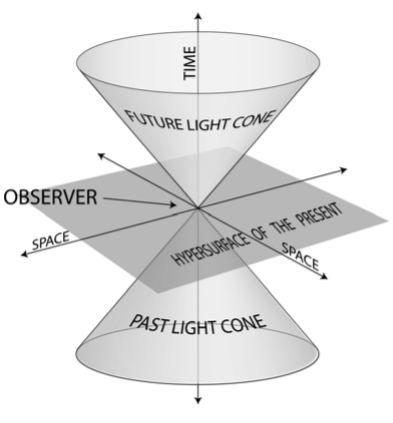
Figure 17.5.1:The light cone in the , , space is defined by the condition and divides space-time into the forward and backward light cones, with and respectively; the interiors of the forward and backward light cones are called absolute future and absolute past.
Inside the light cone
The vertex of the cones represent the present. Locations inside the upper cone represent the future while the past is represented by locations inside the lower cone. Note that inside both the future and past light cones. Thus the space-time interval is real and positive for the future, whereas it is real and negative for the past relative to the vertex of the light cone. A world line is the trajectory a particle follows is a function of time in Minkowski space. In the interior of the future light cone and, since it is real, it can be asserted unambiguously that any point inside this forward cone must occur later than at the vertex of the cone, that is, it is the absolute future. A Lorentz transformation can rotate Minkowski space such that the axis goes through any point within this light cone and then the “world line” is pure time like. Similarly, any point inside the backward light cone unambiguously occurred before the vertex, i.e. it is absolute past.
Outside the Light Cone
Outside of the light cone, has
and thus is imaginary and is called space like. A spacelike plane hypersurface in spatial coordinates is shown for the present time in the unprimed frame. A rotation in Minkowski space can be made to such that the space-like hypersurface now is tilted relative to the hypersurface shown and thus any point outside the light cone can be made to occur later, simultaneous, or earlier than at the vertex depending on the orientation of the space-like hypersurface. This startling situation implies that the time ordering of two points, each outside the others light cone, can be reversed which has profound implications related to the concept of simultaneity and the notion of causality.
For the special case of two events lying on the light cone:
and thus these events are separated by a light ray traveling at velocity . Only events separated by time-like intervals can be connected causally. The world line of a particle must lie within its light cone. The division of intervals into space-like and time-like, because of their invariance, is an absolute concept. That is, it is independent of the frame of reference.
The concept of proper time can be expanded by considering a clock at rest in frame which is moving with uniform velocity with respect to a rest frame . The clock at rest in the frame measures the proper time, then the time observed in the fixed frame can be obtained by looking at the interval . Because of the invariance of the interval, then
That is,
that is which satisfies the normal expression for time dilation, .
Momentum-energy four vector
The previous four-vector discussion can be elegantly exploited using the covariant Minkowski space-time representation. Separating the spatial and time of the differential four vector gives
Remember that the square of the four-dimensional space-time element of length is invariant 17.43, and is simply related to the proper time element . Thus the scalar product
Thus the proper time is an invariant.
The ratio of the four-vector element and the invariant proper time interval , is a four-vector called the four-vector velocity where
where is the particle velocity, and .
The four-vector momentum can be obtained from the four-vector velocity by multiplying it by the scalar rest mass
However,
thus the momentum four vector can be written as
where the vector represents the three spatial components of the relativistic momentum. It is interesting to realize that the Theory of Relativity couples not only the spatial and time coordinates, but also, it couples their conjugate variables linear momentum and total energy, .
An additional feature of this momentum-energy four vector , is that the scalar inner product is invariant to Lorentz transformations and equals in the rest frame
which leads to the well-known equation
The Lorentz transformation matrix can be applied to
The Lorentz invariant four-vector representation is illustrated by applying the Lorentz transformation shown in Figure 17.2.1, which gives, , , , and .
17.6: Lorentz-Invariant Formulation of Lagrangian Mechanics
Parametric Formulation
The Lagrangian and Hamiltonian formalisms in classical mechanics are based on the Newtonian concept of absolute time which serves as the system evolution parameter in Hamilton’s Principle. This approach violates the Special Theory of Relativity. The extended Lagrangian and Hamiltonian formalism is a parametric approach, pioneered by Lanczos[La49], that introduces a system evolution parameter that serves as the independent variable in the action integral, and all the space-time variables are dependent on the evolution parameter . This extended Lagrangian and Hamiltonian formalism renders it to a form that is compatible with the Special Theory of Relativity. The importance of the Lorentz-invariant extended formulation of Lagrangian and Hamiltonian mechanics has been recognized for decades.[La49, Go50, Sy60] Recently there has been a resurgence of interest in the extended Lagrangian and Hamiltonian formalism stimulated by the papers of Struckmeier[Str05, Str08] and this formalism has featured prominently in recent textbooks by Johns[Jo05] and Greiner[Gr10]. This parametric approach develops manifestly-covariant Lagrangian and Hamiltonian formalisms that treat equally all space-time canonical variables. It provides a plausible manifestly-covariant Lagrangian for the one-body system, but serious problems exist extending this to the -body system when . Generalizing the Lagrangian and Hamiltonian formalisms into the domain of the Special Theory of Relativity is of fundamental importance to physics, while the parametric approach gives insight into the philosophy underlying use of variational methods in classical mechanics.[3]
In conventional Lagrangian mechanics, the equations of motion for the generalized coordinates are derived by minimizing the action integral, that is, Hamilton’s Principle.
where denotes the conventional Lagrangian. This approach implicitly assumes the Newtonian concept of absolute time which is chosen to be the independent variable that characterizes the evolution parameter of the system. The actual path the system follows is defined by the extremum of the action integral which leads to the corresponding Euler-Lagrange equations. This assumption is contrary to the Theory of Relativity which requires that the space and time variables be treated equally, that is, the Lagrangian formalism must be covariant.
Extended Lagrangian
Lanczos[La49] proposed making the Lagrangian covariant by introducing a general evolution parameter , and treating the time as a dependent variable on an equal footing with the configuration space variables . That is, the time becomes a dependent variable similar to the spatial variables where . The dynamical system then is described as motion confined to a hypersurface within an extended space where the value of the extended Hamiltonian and the evolution parameter constitute an additional pair of canonically conjugate variables in the extended space. That is, the canonical momentum , corresponding to , is similar to the momentum-energy four vector, equation .
An extended Lagrangian can be defined which can be written compactly as where the index denotes the entire range of space-time variables.
This extended Lagrangian can be used in an extended action functional to give an extended version of Hamilton’s Principle[4]
The conventional action , and extended action , address alternate characterizations of the same underlying physical system, and thus the action principle implies that must hold simultaneously. That is,
As discussed in chapter 9.3, there is a continuous spectrum of equivalent gauge-invariant Lagrangians for which the Euler-Lagrange equations lead to identical equations of motion. Equation 17.57 is satisfied if the conventional and extended Lagrangians are related by
where is a continuous function of and that has continuous second derivatives. It is acceptable to assume that , then the extended and conventional Lagrangians have a unique relation requiring no simultaneous transformation of the dynamical variables. That is, assume
Note that the time derivative of can be expressed in terms of the derivatives by
Thus, for a conventional Lagrangian with variables, the corresponding extended Lagrangian is a function of variables while the conventional and extended Lagrangians are related using equations 17.59, and 17.60.
The derivatives of the relation between the extended and conventional Lagrangians lead to
where since the time derivatives are written explicitly in equations 17.62, 17.64.
Equations 17.63 — 17.64, summed over the extended range of time and spatial dynamical variables, imply
Equation 17.65 can be written in the form
If the extended Lagrangian is homogeneous to first order in the variables , then Euler’s theorem on homogeneous functions trivially implies the relation given in Equation 17.66. Struckmeier[Str08] identified a subtle but important point that if is not homogeneous in , then Equation 17.66 is not an identity but is an implicit equation that is always satisfied as the system evolves according to the solution of the extended Euler-Lagrange equations. Then Equation 17.59 is satisfied without it being a homogeneous form in the velocities . This introduces a new class of non-homogeneous Lagrangians. The relativistic free particle, discussed in example 17.6.1, is a case of a non-homogeneous extended Lagrangian.
Extended generalized momenta
The generalized momentum is defined by
Assume that the definitions of the extended Lagrangian , and the extended Hamiltonian , are related by a Legendre transformation, and are based on variational principles, analogous to the relation that exists between the conventional Lagrangian and Hamiltonian . The Legendre transformation requires defining the extended generalized (canonical) momentum-energy four vector . The momentum components of the momentum-energy four vector are given by the components using Equation 17.63.
The component of the momentum-energy four vector can be derived by recognizing that the right-hand side of Equation 17.64 is equal to . That is, the corresponding generalized momentum , that is conjugate to , is given by
Extended Lagrange equations of motion
By direct analogy with the non-relativistic action integral 17.55, the extremum for the relativistic action integral is obtained using the Euler-Lagrange equations derived from Equation 17.56 where the independent variable is . This implies that for
where the extended generalized force shown on the right-hand side of Equation 17.70, accounts for all forces not included in the potential energy term in the Lagrangian. The extended generalized force can be factored into two terms as discussed in chapter 6, equation . The Lagrange multiplier term includes holonomic constraint forces where the holonomic constraints, which do no work, are expressed in terms of the algebraic equations of holonomic constraint . The term includes the remaining constraint forces and generalized forces that are not included in the Lagrange multiplier term or the potential energy term of the Lagrangian.
For the case where , since , then Equation 17.70 reduces to
These Euler-Lagrange equations of motion 17.70, 17.71 determine the generalized coordinates , plus in terms of the independent variable .
If the holonomic equations of constraint are time independent, that is and if , then the term of the Euler-Lagrange equations simplifies to
One interpretation is to select to be primary. Then is derived from using Equation 17.59 and must satisfy the identity given by Equation 17.66 while the Euler-Lagrange equations containing yield an identity which implies that does not provide an equation of motion in terms of . Conversely, if is chosen to be primary, then is no longer a homogeneous function and Equation 17.66 serves as a constraint on the motion that can be used to deduce , while yields a non-trivial equation of motion in terms of . In both cases the occurrence of a constraint surface results from the fact that the extended space has variables to describe degrees of freedom, that is, one more degree of freedom than required for the actual system.
17.7: Lorentz-invariant formulations of Hamiltonian Mechanics
Extended Canonical Formalism
A Lorentz-invariant formulation of Hamiltonian mechanics can be developed that is built upon the extended Lagrangian formalism assuming that the Hamiltonian and Lagrangian are related by a Legendre transformation. That is,
where the generalized momentum is defined by
Struckmeier[Str08] assumes that the definitions of the extended Lagrangian , and the extended Hamiltonian , are related by a Legendre transformation, and are based on variational principles, analogous to the relation that exists between the conventional Lagrangian and Hamiltonian . The Legendre transformation requires defining the extended generalized (canonical) momentum-energy four vector . The momentum components of the momentum-energy four vector are given by the components using either the conventional or the extended Lagrangians as given in Equation 17.68
The component of the momentum-energy four vector is given by equation
where represents the instantaneous generalized energy of the conventional Hamiltonian at the point , but not the functional form of . That is
Note that does not give the function . Equations 17.68 and give that
The extended Hamiltonian , in an extended phase space, can be defined by the Legendre transformation and the four-vector to be
where the term has been written explicitly as in Equation 17.79. The extended Hamiltonian can carry all the information on the dynamical system that is carried by the extended Lagrangian , if the Hesse matrix is non-singular. That is, if
If the extended Lagrangian is not homogeneous in the velocities , then the extended set of Euler-Lagrange equations is not redundant. Thus equation is not an identity but it can be regarded as an implicit equation that is always satisfied by the extended set of Euler-Lagrange equations. As a result, the Legendre transformation to an extended Hamiltonian exists. That is, equation is identical to the Legendre transform for which was shown to equal zero. Therefore
which means that the extended Hamiltonian directly defines the restricted hypersurface on which the particle motion is confined.
The extended canonical equations of motion, derived using the extended Hamiltonian with the usual Hamiltonian mechanics relations, are:
These canonical equations give that the total derivative of with respect to , is
That is, in contrast to the total time derivative of , the total derivative of the extended Hamiltonian always vanishes, that is, is autonomous which is ideal for use with Hamilton’s equations of motion. The constraints give that , (Equation 17.81) and , (Equation 17.86) implying that the correlation between the extended and conventional Hamiltonians is given by
since only the term with does not cancel in Equation 17.79. Equations 17.81 and 17.90 give that both the left and right-hand sides of Equation 17.90 are zero while Equation 17.86 implies that is a constant of motion, that is, is a cyclic variable for . Formally one can consider the extended Hamiltonian is a constant which equals zero
Equations 17.84, 17.85 imply that form a pair of canonically conjugate variables in addition to the newly-introduced canonically-conjugate variables . Equation 17.90 shows that the motion in the extended phase space is constrained to the surface reflecting the fact that the observed system has one less degree of freedom than used by the extended Hamiltonian.
In summary, the Lorentz-invariant extended canonical formalism leads to Hamilton’s first-order equations of motion in terms of derivatives with respect to , where is related to the proper time for a relativistic system.
Extended Poisson Bracket representation
Struckmeier[Str08] investigated the usefulness of the extended formalism when applied to the Poisson bracket representation of Hamiltonian mechanics. The extended Poisson bracket for two differentiable functions and is defined as
As for the conventional Poisson bracket discussed in chapter 15, the extended Poisson also leads to the fundamental Poisson bracket relations
where . These are identical to the non-extended fundamental Poisson brackets.
The discussion of observables in Hamiltonian mechanics in chapter 15.2.5 can be trivially expanded to the extended Poisson bracket representation. In particular, the total derivative of the function is given by
If commutes with the extended Hamiltonian, that is, the Poisson bracket equals zero, and if , then . That is, the observable is a constant of motion.
Substitute the fundamental variables for gives
where . These are Hamilton’s extended canonical equations of motion expressed in terms of the system evolution parameter . The extended Poisson bracket representation is a trivial extension of the conventional canonical equations presented in chapter 15.3.
Extended canonical transformation and Hamilton-Jacobi theory
Struckmeier[Str08] presented plausible extended versions of canonical transformation and Hamilton-Jacobi theories that can be used to provide a Lorentz-invariant formulation of Hamiltonian mechanics for relativistic one-body systems. A detailed description can be found in Struckmeier[Str08].[5]
Validity of the extended Hamilton-Lagrange formalism
It has been shown that the extended Lagrangian and Hamiltonian formalism, based on the parametric model of Lanczos[La49], leads to a plausible manifestly-covariant approach for the one-body system. The general features developed for handling Lagrangian and Hamiltonian mechanics carry over to the Special Theory of Relativity assuming the use of a non-standard, extended Lagrangian or Hamiltonian. This expansion of the range of validity of the well-known Hamiltonian and Lagrangian mechanics into the relativistic domain is important, and reduces any Lorentz transformation to a canonical transformation. The validity of this extended Hamilton-Lagrange formalism has been criticized, and problems exist extending this approach to the -body system for . For example, as discussed by Goldstein[Go50] and Johns[Jo05], each of the moving bodies have their own world lines and momenta. Defining the total momentum requires knowing simultaneously the momenta of the individual bodies, but simultaneity is body dependent and thus even the total momentum is not a simple four vector. A general method is required that will allow using a manifestly-covariant Lagrangian or Hamiltonian for the -body system. For the one-body system, the extended Hamilton-Lagrange formalism provides a powerful and logical approach to exploit analytical mechanics in the relativistic domain that retains the form of the conventional Lagrangian/Hamiltonian formalisms. Note that Noether’s theorem relating energy and time is readily apparent using the extended formalism.
17.8: The General Theory of Relativity
The Special Theory of Relativity is restricted to inertial frames that are in uniform non-accelerated motion, and are assumed to exist over all of space-time. In 1916 Einstein published the General Theory of Relativity which expands the scope of relativistic mechanics to include non-inertial accelerating frames plus a unified theory of gravitation. The General Theory of Relativity incorporates both the Special Theory of Relativity as well as Newton’s Law of Universal Gravitation. It provides a unified theory of gravitation that is a geometric property of space and time. In particular, the curvature of space-time is directly related to the four-momentum of matter and radiation. Unfortunately, Einstein’s equations of general relativity are nonlinear partial differential equations that are difficult to solve exactly, and the theory requires knowledge of Riemannian geometry that goes beyond the scope of this book. However, it is useful to summarize the fundamental concepts upon which the theory is based, and some of the observable implications since the General Theory of Relativity is an important branch of classical mechanics.
The Fundamental Concepts
The development of general relativity by Einstein was strongly influenced by the following five principles.
Mach’s Principle
The 1883 work “The Science of Mechanics” by the philosopher/physicist, Ernst Mach, criticized Newton’s concept of an absolute frame of reference, and suggested that local physical laws are determined by the large-scale structure of the universe. The concept is that local motion of a rotating frame is determined by the large-scale distribution of matter, that is, relative to the fixed stars. Einstein’s interpretation of Mach’s statement was that the inertial properties of a body is determined by the presence of other bodies in the universe, and he named this concept Mach’s Principle. Mach’s Principle has never been developed into a quantitative physical theory that would explain a mechanism by which the large-scale distribution of matter can produce such an effect.
Equivalence Principle
The equivalence principle comprises closely-related concepts dealing with the equivalence of gravitational and inertial mass. The weak equivalence principle states that the inertial mass and gravitational mass of a body are identical, leading to acceleration that is independent of the nature of the body. This experimental fact usually is attributed to Galileo. Recent measurements have shown that this weak equivalence principle is obeyed to a sensitivity of . Einstein’s equivalence principle states that the outcome of any local non-gravitational experiment, in a freely falling laboratory, is independent of the velocity of the laboratory and its location in space-time. This principle implies that the result of local experiments must be independent of the velocity of the apparatus. Einstein’s equivalence principle has been tested by searching for variations of dimensionless fundamental constants such as the fine structure constant. The strong equivalence principle combines the weak equivalence and Einstein equivalence principles, and implies that the gravitational constant is constant everywhere in the universe. The strong equivalence principle suggests that gravity is geometrical in nature and does not involve any fifth force in nature. Einstein’s General Theory of Relativity satisfies the strong equivalence principle. Tests of the strong equivalence principle have involved searches for variations in the gravitational constant and masses of fundamental particles throughout the life of the universe.
Principle of Covariance
A physical law expressed in a covariant formulation has the same mathematical form in all coordinate systems, and is usually expressed in terms of tensor fields. Maxwell’s equations of electromagnetism are an example of such a covariant formulation. In the Special Theory of Relativity, the Lorentz, rotational, translational and reflection transformations between inertial coordinate frames all are covariant. The covariant quantities are the 4-scalars, and 4-vectors in Minkowski space-time. Einstein recognized that the principle of covariance, that is built into the Special Theory of Relativity, should apply equally to accelerated relative motion in the General Theory of Relativity. He exploited tensor calculus to extend the Lorentz covariance to the more general local covariance in the General Theory of Relativity. The reduction locally of the general metric tensor to the Minkowski metric corresponds to free-falling motion, that is geodesic motion, and thus encompasses gravitation. Unified field theory involves attempts to extend the General Theory of Relativity to incorporate other physical phenomena within a covariant framework in a purely geometric representation in space-time.
Correspondence principle
The Correspondence Principle states that the predictions of any new scientific theory must reduce to the predictions of well established earlier theories under circumstances for which the preceding theory was known to be valid. This also is referred to as the “correspondence limit”. The Correspondence Principle is an important concept used both in quantum mechanics and relativistic mechanics. Einstein’s Special Theory of Relativity satisfies the Correspondence Principle because it reduces to classical mechanics in the limit of velocities small compared to the speed of light. The Correspondence Principle requires that the General Theory of Relativity must reduce to the Special Theory of Relativity for inertial frames, and should approximate Newton’s Theory of Gravitation in weak fields and at low velocities.
Principle of Minimal Gravitational Coupling
The principle of minimal gravitational coupling requires that the total Lagrangian for the field equations of general relativity consist of two additive parts, one part corresponding to the free gravitational Lagrangian, and the other part to external source fields in curved space-time. That is, no terms explicitly containing the curvature of space-time should be added in the extension from the special to general theories of relativity.
Einstein’s postulates for the General Theory of Relativity
Einstein realized that the Equivalence Principle relating the gravitational and inertial masses implies that the constancy of the velocity of light in vacuum cannot hold in the presence of a gravitational field. That is, the Minkowskian line element must be replaced by a more general line element that takes gravity into account. Einstein proposed that the Minkowskian line element in four-dimensional space-time, be replaced by introducing a four-dimensional Riemannian geometrical structure where space, time, and matter are combined. As described by Lanczos[La49], [Har03], [Mu08] this astonishingly bold proposal implies that planetary motion is described as purely a geodesic phenomenon in a certain four-space of Riemannian structure, where the geodesic is the equation of a curve on a manifold for any possible set of coordinates. This implies that the concept of “gravitational force” is discarded, and planetary motion is a manifestation of a pure geodesic phenomenon for forceless motion in a four-dimensional Riemannian structure.
Chapter 5.10 showed that the Lagrangian and Hamiltonian representations of variational mechanics are powerful approaches for determining the equation governing geodesic constrained motion. In addition, these representations are independent of the chosen frame of reference as required by the General Theory of Relativity. Thus variational mechanics is the preeminent theoretical representation of the General Theory of Relativity and the predictions are consistent with the fundamental concepts described in chapter 16.8.
To summarize, the Special Theory of Relativity implies that the Newtonian concepts of absolute frame of reference and separation of space and time are invalid. The General Theory of Relativity goes beyond the Special Theory by implying that the gravitational force, and the resultant planetary motion, can be described as pure geodesic phenomena for forceless motion in a four-dimensional Riemannian structure.
Experimental evidence
The evidence in support of Einstein’s Theory of General Relativity is compelling. The following are typical experimental manifestations of the General Theory of Relativity.
Kepler problem
In 1915 Einstein showed that relativistic mechanics explained the anomalous advance of the perihelion of the planet Mercury, that is, the axes of the elliptical Kepler orbit precess. Example 16.7.1 discusses the analog of this effect for the Bohr-Sommerfeld hydrogen atom.
Deflection of light
Eddington traveled to the island of Príncipe, near Africa, to watch the solar eclipse of 29 May 1919. During the eclipse, he took pictures of the stars in the region around the Sun. According to the theory of general relativity, stars with light rays that passed near the Sun would appear to have been slightly shifted because their light had been curved by the sun’s gravitational field. This effect is noticeable only during eclipses, since otherwise the Sun’s brightness obscures the affected stars. The results confirmed Einstein’s prediction of the deflection of light in a gravitational field which made Einstein famous.
Gravitational lensing
The deflection of light by the gravitational attraction of a massive object situated between a distant star and the observer results in the observation of multiple images of the distant quasar.
Gravitational time dilation and frequency shift
Processes occurring in a high gravitational field are slower than in a weak gravitational field; this is called gravitational time dilation. In addition, light climbing out of a gravitational well is red shifted. The gravitational time dilation has been measured many times and the continued operation of the Global Positioning System provides an ongoing validation. The gravitational red shift has been confirmed in the laboratory using the precise Mössbauer effect in nuclear physics. Tests in stronger gravitational fields are provided by studies of binary pulsars. All of these measurements confirm the general theory of relativity.
Gravitational waves detection
In 1916 Einstein predicted the existence of gravitational waves on the basis of the theory of general relativity. The first implied detection of gravitational waves were made in 1976 by Hulse and Taylor who detected a decrease in the orbital period due to significant energy loss which presumably was associated with emission of gravity waves by the compact neutron star in the binary pulsar . The most compelling direct evidence for observation of a gravitational wave was made on 15 September 2015 by the LIGO Laser Interferometer Gravitational-Wave Observatories. The waveform detected by the two LIGO observatories matched the predictions of General Relativity for gravitational waves emanating from the inward spiral plus merger of a pair of black holes of around 36 and 29 solar masses, followed by the resultant binary black hole. The gravitational wave emitted by this cataclysmic merger reached Earth as a ripple in space-time that changed the length of the 4 LIGO arm by a thousandth of the width of the proton. The gravitational energy emitted was solar masses. A second observation of gravitational waves was made on 26 December 2015, and four similar observations were made during 2017. The detection of such minuscule changes in space-time is a truly remarkable achievement. This direct detection of gravitational waves resulted in the award of the 2017 Nobel Prize to Rainer Weiss, Barry Barish, and Kip Thorne.
Black holes
If the mass to radius ratio of a massive object becomes sufficiently large, general relativity predicts formation of a black hole, which is a region of space from which neither light nor matter can escape. A supermassive black hole, with a mass that is solar masses, is thought to have played an important role in formation of the M87 galaxy. This black hole at the core of the massive elliptical M87 galaxy was observed April 2017 by the Event Horizon Telescope (EHT). Figure 17.8.1 shows a polarized light image of this black hole, revealing a ring-like structure consistent with synchrotron emission from relativistic electrons that are gyrating around the inner edge of a vortex of magnetic field lines in the vicinity of the event horizon. (The Astrophysical Journal Letters, 910:L12, 20 March 2021).
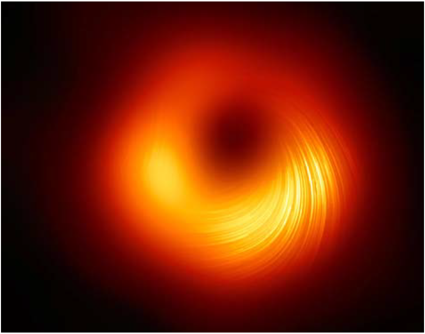
Figure 17.8.1:Polarized-light image of the M87 black hole
17.9: Implications of Relativistic Theory to Classical Mechanics
Einstein’s theories of relativity have had an enormous impact on twentieth century physics and the philosophy of science. Relativistic mechanics is crucial to an understanding of the physics of the atom, nucleus and the substructure of the nucleons, but the impacts are minimal in everyday experience. As a consequence the enormous philosophical implications of Einstein’s theories of relativity may not be as readily apparent as other major developments during the 20 century. In spite of this, it is important to be cognizant of the consequences of these theories of nature. The Special Theory of Relativity replaces Newton’s Laws of motion; i.e. Newton’s law is only an approximation applicable for low velocities. The General Theory of Relativity replaces Newton’s Law of Gravitation and provides a natural explanation of the equivalence principle. Einstein’s theories of relativity imply a profound and fundamental change in the view of the separation of space, time, and mass, that contradicts the basic tenets that are the foundation of Newtonian mechanics. The Newtonian concepts of absolute frame of reference, plus the separation of space, time, and mass, are invalid at high velocities. Lagrangian and Hamiltonian variational approaches to classical mechanics provide the formalism necessary for handling relativistic mechanics. The present chapter has shown that logical extensions of Lagrangian and Hamiltonian mechanics lead to the relativistically-invariant extended Lagrangian and Hamiltonian formulations of mechanics which is adequate for handling one-body systems within the Special Theory of Relativity. However, major unsolved problems remain applying these formulations to systems having more than one body.
17.E: Relativistic Mechanics (Exercises)
A relativistic snake of proper length 100 is traveling to the right across a butcher’s table at . You hold two meat cleavers, one in each hand which are 100 apart. You strike the table simultaneously with both cleavers at the moment when the left cleaver lands just behind the tail of the snake. You rationalize that since the snake is moving with , then the length of the snake is Lorentz contracted by the factor and thus the Lorentz-contracted length of the snake is 80 and thus will not be harmed. However, the snake reasons that relative to it the cleavers are moving at and thus are only 80 apart when they strike the 100 long snake and thus it will be severed. Use the Lorentz transformation to resolve this paradox.
Explain what is meant by the following statement: “Lorentz transformations are orthogonal transformations in Minkowski space.”
Which of the following are invariant quantities in space-time?
Energy
Momentum
Mass
Force
Charge
The length of a vector
The length of a four-vector
What does it mean for two events to have a spacelike interval? What does it mean for them to have a timelike interval? Draw a picture to support your answer. In which case can events be causally connected?
A supply rocket flies past two markers on the Space Station that are 50 apart in a time of 0.2 as measured by an observer on the Space station.
What is the separation of the two markers as seen by the pilot riding in the supply rocket?
What is the elapsed time as measured by the pilot in the supply rocket?
What are the speeds calculated by the observer in the Space Station and the pilot of the supply rocket?
The Compton effect involves a photon of incident energy being scattered by an electron of mass which initially is stationary. The photon scattered at an angle with respect to the incident photon has a final energy . Using the special theory of relativity derive a formula that related and to .
Pair creation involves production of an electron-positron pair by a photon. Show that such a process is impossible unless some other body, such as a nucleus, is involved. Suppose that the nucleus has a mass and the electron mass . What is the minimum energy that the photon must have in order to produce an electron-positron pair?
A meson of rest energy 494 decays into a meson of rest energy 106 and a neutrino of zero rest energy. Find the kinetic energies of the meson and the neutrino into which the meson decays while at rest.
17.S: Relativistic Mechanics (Summary)
Special Theory of Relativity
The Special Theory of Relativity is based on Einstein’s postulates;
The laws of nature are the same in all inertial frames of reference.
The velocity of light in vacuum is the same in all inertial frames of reference.
For a primed frame moving along the axis with velocity Einstein’s postulates imply the following Lorentz transformations between the moving (primed) and stationary (unprimed) frames
where the Lorentz factor
Lorentz transformations were used to illustrate Lorentz contraction, time dilation, and simultaneity. An elementary review was given of relativistic kinematics including discussion of velocity transformation, linear momentum, center-of-momentum frame, forces and energy.
Geometry of space-time
The concepts of four-dimensional space-time were introduced. A discussion of four-vector scalar products introduced the use of contravariant and covariant tensors plus the Minkowski metric where the scalar product was defined. The Minkowski representation of space time and the momentum-energy four vector also were introduced.
Lorentz-invariant formulation of Lagrangian mechanics
The Lorentz-invariant extended Lagrangian formalism, developed by Struckmeier[Str08], based on the parametric approach pioneered by Lanczos[La49], provides a viable Lorentz-invariant extension of conventional Lagrangian mechanics that is applicable for one-body motion in the realm of the Special Theory of Relativity.
Lorentz-invariant formulation of Hamiltonian mechanics
The Lorentz-invariant extended Hamiltonian formalism, developed by Struckmeier based on the parametric approach pioneered by Lanczos, was introduced. It provides a viable Lorentz-invariant extension of conventional Hamiltonian mechanics that is applicable for one-body motion in the realm of the Special Theory of Relativity. In particular, it was shown that the Lorentz-invariant extended Hamiltonian is conserved making it ideally suited for solving complicated systems using Hamiltonian mechanics via use of the Poisson-bracket representation of Hamiltonian mechanics, canonical transformations, and the Hamilton-Jacobi techniques.
The General Theory of Relativity
An elementary summary was given of the fundamental concepts of the General Theory of Relativity and the resultant unified description of the gravitational force plus planetary motion as geodesic motion in a four-dimensional Riemannian structure. Variational mechanics were shown to be ideally suited to applications of the General Theory of Relativity.
Philosophical implications
Newton’s equations of motion, and his Law of Gravitation, that reigned supreme from 1687 to 1905, have been toppled from the throne by Einstein’s theories of relativistic mechanics. By contrast, the complete independence to coordinate frames in Lagrangian, and Hamiltonian formulations of classical mechanics, plus the underlying Principle of Least Action, are equally valid in both the relativistic and non-relativistic regimes. As a consequence, relativistic Lagrangian and Hamiltonian formulations underlie much of modern physics, especially quantum physics, which explains why relativistic mechanics plays such an important role in classical dynamics.
Note that, until recently, the rest mass was denoted by and the relativistic mass was referred to as . Modern texts denote the rest mass by and the relativistic mass by . This book follows the modern nomenclature for rest mass to avoid confusion.
Older textbooks, such as all editions of Marion, and the first two editions of Goldstein, use the Euclidean Poincaré 4-dimensional space-time with the imaginary time axis . About half the scientific community, and modern physics textbooks including this textbook, and the 3 edition of Goldstein, use the Bjorken - Drell , sign convention given in Equation 17.38 where , and are the spatial coordinates. The other half of the community, including mathematicians and gravitation physicists, use the opposite , sign convention. Further confusion is caused by a few books that assign the time axis to be rather than .
Chapters 17.6 and 17.7 reproduce the Struckmeier presentation.[Str08]
These formula involve total and partial derivatives with respect to both time, and parameter . For clarity, the derivatives are written out in full because Lanczos[La49] and Johns[Jo05] use the opposite convention for the dot and prime superscripts as abbreviations for the differentials with respect to and . The blackboard bold format is used to designate the extended versions of the action , Lagrangian and Hamiltonian .
Note that Greiner[Gr10] includes a reproduction of the Struckmeier paper[Str08].