6. Lagrangian Dynamics - Variational Principles in Classical Mechanics

6.1: Introduction to Lagrangian Dynamics¶

Newtonian mechanics is based on vector observables such as momentum and force, and Newton’s equations of motion can be derived if the forces are known. However, Newtonian mechanics becomes difficult for many-body systems when constraint forces apply. The alternative algebraic Lagrangian mechanics approach is based on the concept of scalar energies which circumvent many of the difficulties in handling constraint forces and many-body systems.

The Lagrangian approach to classical dynamics is based on the calculus of variations introduced in chapter 5. It was shown that the calculus of variations determines the function $y_i(x)$ such that the scalar functional

F = \int^{x_2}_{x_1} \sum^n_i f[y_i (x), y^{\prime}_i (x); x] dx \tag{6.1}

is an extremum, that is, a maximum or minimum. Here $x$ is the independent variable, $y_i(x)$ are the $n$ dependent variables, and their derivatives $y^{\prime}_i \equiv \frac{dy_i}{dx}$ , where $i = 1, 2, 3, ..n$ . The function $f [ y_i(x), y^{\prime}_i (x); x]$ has an assumed dependence on $y_i$ , $y^{\prime}_i$ and $x$ . The calculus of variations determines the functional dependence of the dependent variables $y_i(x)$ on the independent variable $x$ , that is needed to ensure that $F$ is an extremum. For $n$ independent variables, $F$ has a stationary point, which is presumed to be an extremum, that is determined by solution of Euler’s differential equations

\frac{d}{dx}\frac{\partial f}{\partial y_{i}^{\prime }}-\frac{\partial f}{ \partial y_{i}}=0\tag{6.2}

If the coordinates $y_{i}(x)$ are independent, then the Euler equations, 6.2, for each coordinate $i$ are independent. However, for constrained motion, the constraints lead to auxiliary conditions that correlate the coordinates. As shown in chapter 5, a transformation to independent generalized coordinates can be made such that the correlations induced by the constraint forces are embedded into the choice of the independent generalized coordinates. The use of generalized coordinates in Lagrangian mechanics simplifies derivation of the equations of motion for constrained systems. For example, for a system of $n$ coordinates, that involves $m$ holonomic constraints, there are $s=n-m$ independent generalized coordinates. For such holonomic constrained motion, it will be shown that the Euler equations can be solved using either of the following three alternative ways.

The minimal set of generalized coordinates approach involves finding a set of $s=n-m$ independent generalized coordinates $q_{i}$ that satisfy the assumptions underlying 6.2. These generalized coordinates can be determined if the $m$ equations of constraint are holonomic, that is, related by algebraic equations of constraint

g_{k}(q_{i};x)=0\tag{6.3}

where $k=1,2,3,\dots .m.$ These equations uniquely determine the relationship between the $n$ correlated coordinates. This method has the advantage that it reduces the system of $n$ coordinates, subject to $m$ constraints, to $s=n-m$ independent generalized coordinates which reduces the dimension of the problem to be solved. However, it does not explicitly determine the forces of constraint which are effectively swept under the rug.

The Lagrange multipliers approach takes account of the correlation between the $n$ coordinates and $m$ holonomic constraints by introducing the Lagrange multipliers $\lambda _{k}(x)$ . These $n$ generalized coordinates $q_{i}$ are correlated by the $m$ holonomic constraints.

\frac{d}{dx}\frac{\partial f}{\partial q_{i}^{\prime }}-\frac{\partial f}{ \partial q_{i}}=\sum_{k}^{m}\lambda _{k}\left( x\right) \frac{\partial g_{k} }{\partial q_{i}}\tag{6.4}

where $i=1,2,3,\dots n$ . The Lagrange multiplier approach has the advantage that Euler’s calculus of variations automatically use the $n$ Lagrange equations, plus the $m$ equations of constraint, to explicitly determine both the $n$ coordinates $q_{i}$ plus the $m$ forces of constraint which are related to the Lagrange multipliers $\lambda _{k}$ as given in Equation 6.4. Chapter 6.2 shows that the $\sum_{k}^{m}\lambda _{k}\left( x\right) \frac{\partial g_{k}}{\partial y_{i}}$ terms are directly related to the holonomic forces of constraint.

The generalized force approach incorporates the forces of constraint explicitly as will be shown in chapter 6.5.4. Incorporating the constraint forces explicitly allows use of holonomic, non-holonomic, and non-conservative constraint forces.

Understanding the Lagrange formulation of classical mechanics is facilitated by use of a simple non-rigorous plausibility approach that is based on Newton’s laws of motion. This introductory plausibility approach will be followed by two more rigorous derivations of the Lagrangian formulation developed using either d’Alembert Principle or Hamiltons Principle. These better elucidate the physics underlying the Lagrange and Hamiltonian analytic representations of classical mechanics. In 1788 Lagrange derived his equations of motion using the differential d’Alembert Principle, that extends to dynamical systems the Bernoulli Principle of infinitessimal virtual displacements and virtual work. The other approach, developed in 1834, uses the integral Hamilton’s Principle to derive the Lagrange equations. Hamilton’s Principle is discussed in more detail in chapter 9. Euler’s variational calculus underlies d’Alembert’s Principle and Hamilton’s Principle since both are based on the philosophical belief that the laws of nature prefer economy of motion. Chapters $6.2-6.5$ show that both d’Alembert’s Principle and Hamilton’s Principle lead to the Euler-Lagrange equations. This will be followed by a series of examples that illustrate the use of Lagrangian mechanics in classical mechanics.

6.2: Newtonian plausibility argument for Lagrangian mechanics¶

Insight into the physics underlying Lagrange mechanics is given by showing the direct relationship between Newtonian and Lagrangian mechanics. The variational approaches to classical mechanics exploit the first-order spatial integral of the force, equation (2.4.8), which equals the work done between the initial and final conditions. The work done is a simple scalar quantity that depends on the initial and final location for conservative forces. Newton’s equation of motion is

\tag{6.5} \mathbf{F}=\frac{d\mathbf{p}}{dt}

The kinetic energy is given by

\tag{6.6} T=\frac{1}{2}mv^{2}=\frac{\mathbf{p}\cdot \mathbf{p}}{2m}=\frac{p_{x}^{2}}{2m }+\frac{p_{y}^{2}}{2m}+\frac{p_{z}^{2}}{2m} \notag

It can be seen that

\tag{6.7} \frac{\partial T}{\partial \dot{x}}=p_{x}

and

\tag{6.8} \frac{d}{dt}\frac{\partial T}{\partial \dot{x}}=\frac{dp_{x}}{dt}=F_{x}

Consider that the force, acting on a mass $m,$ is arbitrarily separated into two components, one part that is conservative, and thus can be written as the gradient of a scalar potential $U$ , plus the excluded part of the force, $F^{EX}$ . The excluded part of the force $F^{EX}$ could include non-conservative frictional forces as well as forces of constraint which may be conservative or non-conservative. This separation allows the force to be written as

\tag{6.9} \mathbf{F}=-\mathbf{\nabla }U+\mathbf{F}^{EX}

Along each of the $x_{i}$ axes,

\tag{6.10} \frac{d}{dt}\frac{\partial T}{\partial \dot{x}_{i}}=-\frac{\partial U}{ \partial x_{i}}+F_{x_{i}}^{EX}

Equation 6.10 can be extended by transforming the cartesian coordinate $x_{i}$ to the generalized coordinates $q_{i}.$

Define the standard Lagrangian to be the difference between the kinetic energy and the potential energy, which can be written in terms of the generalized coordinates $q_{i}$ as

\tag{6.11} L(q_{i},\dot{q}_{i})\equiv T(\dot{q}_{i})-U(q_{i})

Assume that the potential is only a function of the generalized coordinates $q_{i},$ that is $\frac{\partial U}{\partial \dot{q}_{i}}=0,$ then

\tag{6.12} \frac{\partial L}{\partial \dot{q}_{i}}=\frac{\partial T}{\partial \dot{q} _{i}}+\frac{\partial U}{\partial \dot{q}_{i}}=\frac{\partial T}{\partial \dot{q}_{i}}

Using the above equations allows Newton’s equation of motion 6.10 to be expressed as

\tag{6.13} \frac{d}{dt}\frac{\partial L}{\partial \dot{q}_{i}}-\frac{\partial L}{ \partial q_{i}}=F_{q_{i}}^{EX}

The excluded force $F_{q_{i}}^{EX}$ can be partitioned into a holonomic constraint force $F_{q_{i}}^{HC},$ plus any remaining excluded forces $F^{EXC},$ as given by

\tag{6.14} F_{q_{i}}^{EX}=F_{q_{i}}^{HC}+F^{EXC}

A comparison of equations 6.13 and $(6.1.4)$ shows that the holonomic constraint forces $F_{q_{i}}^{HC},$ that are contained in the excluded force $F^{EX},$ can be identified with the Lagrange multiplier term in equation $(6.1.4)$ .

\tag{6.15} F_{q_{i}}^{HC}\equiv \sum_{k}^{m}\lambda _{k}\left( t\right) \frac{\partial g_{k}}{\partial q_{i}}

That is the Lagrange multiplier terms can be used to account for holonomic constraint forces $F_{q_{i}}^{HC}$ . Thus Equation 6.13 can be written as

\tag{6.16} \frac{d}{dt}\frac{\partial L}{\partial \dot{q}_{i}}-\frac{\partial L}{ \partial q_{i}}=\sum_{k}^{m}\lambda _{k}\left( t\right) \frac{\partial g_{k} }{\partial q_{i}}+F_{q_{i}}^{EXC}

where the Lagrange multiplier term accounts for holonomic constraint forces, and $F_{q_{i}}^{EXC}$ includes all the remaining forces that are not accounted for by the scalar potential $U$ , or the Lagrange multiplier terms $F_{q_{i}}^{HC}$ .

For holonomic, conservative forces it is possible to absorb all the forces into the potential $U$ plus the Lagrange multiplier term, that is $F_{q_{i}}^{EXC}=0.$ Moreover, the use of a minimal set of generalized coordinates allows the holonomic constraint forces to be ignored by explicitly reducing the number of coordinates from $n$ dependent coordinates to $s=n-m$ independent generalized coordinates. That is, the correlations due to the constraint forces are embedded into the generalized coordinates. Then Equation 6.17 reduces to the basic Euler differential equations.

\tag{6.17} \frac{d}{dt}\frac{\partial L}{\partial \dot{q}_{i}}-\frac{\partial L}{ \partial q_{i}}=0

Note that Equation 6.17 is identical to Euler’s equation (5.8.1), if the independent variable $x$ is replaced by time $t$ . Thus Newton’s equation of motion are equivalent to minimizing the action integral $S= \int_{t_{1}}^{t_{2}}Ldt$ , that is

\tag{6.18} \delta S=\delta \int_{t_{1}}^{t_{2}}L(q_{i},\dot{q}_{i};t)dt=0

which is Hamilton’s Principle. Hamilton’s Principle underlies many aspects of physics as discussed in chapter 9, and is used as the starting point for developing classical mechanics. Hamilton’ Principle was postulated 46 years after Lagrange introduced Lagrangian mechanics.

The above plausibility argument, which is based on Newtonian mechanics, illustrates the close connection between the vectorial Newtonian mechanics and the algebraic Lagrangian mechanics approaches to classical mechanics.

6.3: Lagrange Equations from d’Alembert’s Principle¶

d’Alembert’s Principle of virtual work¶

The Principle of Virtual Work provides a basis for a rigorous derivation of Lagrangian mechanics. Bernoulli introduced the concept of virtual infinitessimal displacement of a system mentioned in chapter 5.9.1. This refers to a change in the configuration of the system as a result of any arbitrary infinitessimal instantaneous change of the coordinates $\delta \mathbf{r}_{i},$ that is consistent with the forces and constraints imposed on the system at the instant $t$ . Lagrange’s symbol $\delta$ is used to designate a virtual displacement which is called “virtual” to imply that there is no change in time $t$ , i.e. $\delta t=0$ . This distinguishes it from an actual displacement $d\mathbf{r} _{i}$ of body $i$ during a time interval $dt$ when the forces and constraints may change.

Suppose that the system of $n$ particles is in equilibrium, that is, the total force on each particle $i$ is zero. The virtual work done by the force $\mathbf{F}_{i}$ moving a distance $\delta \mathbf{r}_{i}$ is given by the dot product $\mathbf{F}_{i}\cdot \delta \mathbf{r}_{i}$ . For equilibrium, the sum of all these products for the $N$ bodies also must be zero

\tag{6.18}\sum_{i}^{N}\mathbf{F}_{i}\cdot \delta \mathbf{r}_{i}=0

Decomposing the force $\mathbf{F}_{i}$ on particle $i$ into applied forces $\mathbf{F}_{i}^{A}$ and constraint forces $\mathbf{f}_{i}^{C}$ gives

\tag{6.19} \sum_{i}^{N}\mathbf{F}_{i}^{A}\cdot \delta \mathbf{r}_{i}+\sum_{i}^{N} \mathbf{f}_{i}^{C}\cdot \delta \mathbf{r}_{i}=0

The second term in Equation 6.19 can be ignored if the virtual work due to the constraint forces is zero. This is rigorously true for rigid bodies and is valid for any forces of constraint where the constraint forces are perpendicular to the constraint surface and the virtual displacement is tangent to this surface. Thus if the constraint forces do no work, then 6.19 reduces to

\tag{6.20} \sum_{i}^{N}\mathbf{F}_{i}^{A}\cdot \delta \mathbf{r}_{i}=0

This relation is the Bernoulli’s Principle of Static Virtual Work and is used to solve problems in statics.

Bernoulli introduced dynamics by using Newton’s Law to related force and momentum.

\tag{6.21} \mathbf{F}_{i}=\mathbf{ \dot{p}}_{i}

Equation 6.21 can be rewritten as

\mathbf{F}_{i}-\mathbf{\dot{p}}_{i}=0\tag{6.22}

In 1742, d’Alembert developed the Principle of Dynamic Virtual Work in the form

\sum^N_i (\mathbf{F}_i-\mathbf{\dot{p}}_i) \cdot \delta \mathbf{r}_i = 0 \tag{6.23}

Using equations 6.19 plus 6.23 gives

\sum^N_i (\mathbf{F}^A_i-\mathbf{\dot{p}}_i) \cdot \delta \mathbf{r}_i + \sum^N_i (\mathbf{f}^C_i \cdot \delta \mathbf{r}_i = 0 \tag{6.24}

For the special case where the forces of constraint are zero, then Equation 6.24 reduces to d’Alembert’s Principle

\tag{6.25} \sum_{i}^{N}(\mathbf{F}_{i}^{A}-\mathbf{ \dot{p}}_{i})\cdot \delta \mathbf{r}_{i}=0

d’Alembert’s Principle, by a stroke of genius, cleverly transforms the principle of virtual work from the realm of statics to dynamics. Application of virtual work to statics primarily leads to algebraic equations between the forces, whereas d’Alembert’s principle applied to dynamics leads to differential equations.

Transformation to generalized coordinates¶

In classical mechanical systems the coordinates $\delta \mathbf{r}_{i}$ usually are not independent due to the forces of constraint and the constraint-force energy contributes to Equation 6.24. These problems can be eliminated by expressing d’Alembert’s Principle in terms of virtual displacements of $n$ independent generalized coordinates $q_{i \text{ }}$ of the system for which the constraint force term $\sum_{i}^{n} \mathbf{f}_{i}^{C}\cdot \delta \mathbf{q}_{i}=0$ . Then the individual variational coefficients $\delta q_{i}$ are independent and $(\mathbf{F} _{i}^{A}-\mathbf{\dot{p}}_{i})\cdot \delta \mathbf{q}_{i}=0$ can be equated to zero for each value of $i$ .

The transformation of the $N$ -body system to $n$ independent generalized coordinates $q_{k}$ can be expressed as

\tag{6.26} \mathbf{r}_{i}=\mathbf{r}_{i}(q_{1},q_{2},q_{3} \dots ,q_{n},t)

Assuming $n$ independent coordinates, then the velocity $\mathbf{v}_{i}$ can be written in terms of general coordinates $q_{k}$ using the chain rule for partial differentiation.

\tag{6.27} \mathbf{v}_{i}\equiv \frac{d\mathbf{r}_{i}}{dt}=\sum_{j}^{n}\frac{\partial \mathbf{r}_{i}}{ \partial q_{j}}\dot{q}_{j}+\frac{\partial \mathbf{r}_{i}}{\partial t}

The arbitrary virtual displacement $\delta \mathbf{r}_{i}$ can be related to the virtual displacement of the generalized coordinate $\delta q_{j}$ by

\tag{6.28} \delta \mathbf{r}_{i}=\sum_{j}^{n}\frac{\partial \mathbf{r}_{i}}{\partial q_{j}}\delta q_{j}

Note that by definition, a virtual displacement considers only displacements of the coordinates, and no time variation $\delta t$ is involved.

The above transformations can be used to express d’Alembert’s dynamical principle of virtual work in generalized coordinates. Thus the first term in d’Alembert’s Dynamical Principle, 6.25 becomes

\tag{6.29} \sum_{i}^{n}\mathbf{F}_{i}^{A}\cdot \delta \mathbf{r}_{i}=\sum_{i,j}^{n} \mathbf{F}_{i}^{A}\cdot \frac{\partial \mathbf{r}_{i}}{\partial q_{j}}\delta q_{j}=\sum_{j}^{n}Q_{j}\delta q_{j}

where $Q_{j}$ are called components of the generalized force,^[1] defined as

\tag{6.30} Q_{j}\equiv \sum_{i}^{n}\mathbf{F}_{i}^{A}\cdot \frac{\partial \mathbf{r}_{i}}{\partial q_{j}}

Note that just as the generalized coordinates $q_{j}$ need not have the dimensions of length, so the $Q_{j}$ do not necessarily have the dimensions of force, but the product $Q_{j}\delta q_{j}$ must have the dimensions of work. For example, $Q_{j}$ could be torque and $\delta q_{j}$ could be the corresponding infinitessimal rotation angle.

The second term in d’Alembert’s Principle 6.25 can be transformed using Equation 6.28

\tag{6.31} \sum_{i}^{n}\mathbf{\dot{p}}_{i}\cdot \delta \mathbf{r}_{i}=\sum_{i}^{n}m_{i} \mathbf{\ddot{r}}_{i}\cdot \delta \mathbf{r}_{i}=\left( \sum_{i}^{n}m_{i} \mathbf{\ddot{r}}_{i}\cdot \frac{\partial \mathbf{r}_{i}}{\partial q_{j}} \right) \delta q_{j}

The right-hand side of 6.31 can be rewritten as

\tag{6.32} \left( \sum_{i}^{n}m_{i}\mathbf{\ddot{r}}_{i}\cdot \frac{\partial \mathbf{r} _{i}}{\partial q_{j}}\right) \delta q_{j}=\sum_{i}^{n}\left\{ \frac{d}{dt} \left( m_{i}\mathbf{\dot{r}}_{i}\cdot \frac{\partial \mathbf{r}_{i}}{ \partial q_{j}}\right) -m_{i}\mathbf{\dot{r}}_{i}\cdot \frac{d}{dt}\left( \frac{\partial \mathbf{r}_{i}}{\partial q_{j}}\right) \right\} \delta q_{j}

Note that Equation 6.27 gives that

\tag{6.33} \frac{\partial \mathbf{v}_{i}}{\partial \dot{q}_{j}}=\frac{\partial \mathbf{r }_{i}}{\partial q_{j}}

therefore the first right-hand term in 6.32 can be written as

\tag{6.34} \frac{d}{dt}\left( m_{i}\mathbf{\dot{r}}_{i}\cdot \frac{\partial \mathbf{r} _{i}}{\partial q_{j}}\right) =\frac{d}{dt}\left( m_{i}\mathbf{v}_{i}\cdot \frac{\partial \mathbf{v}_{i}}{\partial \dot{q}_{j}}\right)

The second right-hand term in 6.32 can be rewritten by interchanging the order of the differentiation with respect to $t$ and $q_{j}$

\tag{6.35} \frac{d}{dt}\left( \frac{\partial \mathbf{r}_{i}}{\partial q_{j}}\right) = \frac{\partial \mathbf{v}_{i}}{\partial q_{j}}

Substituting 6.34 and 6.35 into 6.32 gives

\tag{6.36} \sum_{i}^{n}\mathbf{\dot{p}}_{i}\cdot \delta \mathbf{r}_{i}=\left( \sum_{i}^{n}m_{i}\mathbf{\ddot{r}}_{i}\cdot \frac{\partial \mathbf{r}_{i}}{ \partial q_{j}}\right) \delta q_{j}=\sum_{i}^{N}\left\{ \frac{d}{dt}\left( m_{i}\mathbf{v}_{i}\cdot \frac{\partial \mathbf{v}_{i}}{\partial \dot{q}_{j}} \right) -m_{i}\mathbf{v}_{i}\cdot \frac{\partial \mathbf{v}_{i}}{\partial q_{j}}\right\} \delta q_{j}

Inserting 6.29 and 6.36 into d’Alembert’s Principle 6.25 leads to the relation

\tag{6.37} \sum_{i}^{n}(\mathbf{F}_{i}^{A}-\mathbf{\dot{p}}_{i})\cdot \delta \mathbf{r} _{i}=-\sum_{j}^{N}\left\{ \frac{d}{dt}\left( \frac{\partial }{\partial \dot{q }_{j}}\left( \sum_{i}\frac{1}{2}m_{i}v_{i}^{2}\right) \right) -\frac{ \partial }{\partial q_{j}}\left( \sum_{i}^{N}\frac{1}{2}m_{i}v_{i}^{2} \right) -Q_{j}\right\} \delta q_{j}=0

The $\sum_{i}^{n}\frac{1}{2}m_{i}v_{i}^{2}$ term can be identified with the system kinetic energy $T$ . Thus d’Alembert Principle reduces to the relation

\tag{6.38} \sum_{j}^{N}\left[ \left\{ \frac{d}{dt}\left( \frac{\partial T}{\partial \dot{q}_{j}}\right) -\frac{\partial T}{\partial q_{j}}\right\} -Q_{j}\right] \delta q_{j}=0

For cartesian coordinates $T$ is a function only of velocities $(\dot{x}, \dot{y},\dot{z})$ and thus the term $\frac{\partial T}{\partial q_{j}}=0.$ However, as discussed in appendix 19.3, for curvilinear coordinates $\frac{\partial T}{\partial q_{j}}\neq 0$ due to the curvature of the coordinates as is illustrated for polar coordinates where $\mathbf{v=}\dot{r} \mathbf{\hat{r}}+r\dot{\theta}\mathbf{\hat{\theta}}$ .

\tag{6.39} \left\{ \frac{d}{dt}\left( \frac{\partial T}{\partial \dot{q}_{j}}\right) - \frac{\partial T}{\partial q_{j}}\right\} =Q_{j}

where $n\geq j\geq 1$ . That is, this leads to $n$ Euler-Lagrange equations of motion for the generalized forces $Q_{j}$ . As discussed in chapter $5.8,$ when $m$ holonomic constraint forces apply, it is possible to reduce the system to $s=n-m$ independent generalized coordinates for which Equation 6.25 applies.

In 1687 Leibniz proposed minimizing the time integral of his “vis viva", which equals $2T.$ That is,

\tag{6.40} \delta \int_{t_{1}}^{t_{2}}Tdt=0

The variational Equation 6.39 accomplishes the minimization of Equation 6.40. It is remarkable that Leibniz anticipated the basic variational concept prior to the birth of the developers of Lagrangian mechanics, i.e., d’Alembert, Euler, Lagrange, and Hamilton.

Lagrangian¶

The handling of both conservative and non-conservative generalized forces $Q_{j}$ is best achieved by assuming that the generalized force $Q_{j}=\sum_{i}^{n}\mathbf{F}_{i}^{A}\cdot \frac{\partial \mathbf{\bar{r}}_{i} }{\partial q_{j}}$ can be partitioned into a conservative velocity-independent term, that can be expressed in terms of the gradient of a scalar potential, $-\mathbf{\nabla }U_{i},$ plus an excluded generalized force $Q_{j}^{EX}$ which contains the non-conservative, velocity-dependent, and all the constraint forces not explicitly included in the potential $U_{j}$ . That is,

\tag{6.41} Q_{j}=-\mathbf{\nabla }U_{j}+Q_{j}^{EX}

Inserting 6.41 into 6.38, and assuming that the potential $U$ is velocity independent, allows 6.38 to be rewritten as

\tag{6.42} \sum_{j}\left[ \left\{ \frac{d}{dt}\left( \frac{\partial (T-U)}{\partial \dot{q}_{j}}\right) -\frac{\partial (T-U)}{\partial q_{j}}\right\} -Q_{j}^{EX}\right] \delta q_{j}=0

The standard definition of the Lagrangian is

\tag{6.43} L\equiv T-U

then 6.42 can be written as

\tag{6.44} \sum_{j}^{N}\left[ \left\{ \frac{d}{dt}\left( \frac{\partial L}{\partial \dot{q}_{j}}\right) -\frac{\partial L}{\partial q_{j}}\right\} -Q_{j}^{EX} \right] \delta q_{j}=0

Note that if all the generalized coordinates are independent, then the square bracket terms are zero for each value of $j$ , which leads to the general Euler-Lagrange equations of motion.

\tag{6.45} \left\{ \frac{d}{dt}\left( \frac{\partial L}{\partial \dot{q}_{j}}\right) - \frac{\partial L}{\partial q_{j}}\right\} =Q_{j}^{EX}

where $n\geq j\geq 1$ .

Chapter 6.5.3 will show that the holonomic constraint forces can be factored out of the generalized force term $Q_{j}^{EX}$ which simplifies derivation of the equations of motion using Lagrangian mechanics. The general Euler-Lagrange equations of motion are used extensively in classical mechanics because conservative forces play a ubiquitous role in classical mechanics.

6.4: Lagrange equations from Hamilton’s Principle¶

Lagrange equations from Hamilton’s Action Principle¶

Hamilton published two papers in 1834 and 1835, announcing a fundamental new dynamical principle that underlies both Lagrangian and Hamiltonian mechanics. Hamilton was seeking a theory of optics when he developed Hamilton’s Action Principle, plus the field of Hamiltonian mechanics, both of which play a crucial role in classical mechanics and modern physics. Hamilton’s Action Principle states “dynamical systems follow paths that minimize the time integral of the Lagrangian”. That is, the action functional $S$

S=\int_{t_{1}}^{t_{2}}L(\mathbf{q, \dot{q},}t)dt

has a minimum value for the correct path of motion. Hamilton’s Action Principle can be written in terms of a virtual infinitessimal displacement $\delta ,$ as

\delta S=\delta \int_{t_{1}}^{t_{2}}Ldt=0

Variational calculus therefore implies that a system of $s$ independent generalized coordinates must satisfy the basic Lagrange-Euler equations

\frac{d}{dt}\frac{\partial L}{\partial \dot{q}_{j}}-\frac{\partial L}{ \partial q_{j}}=0

Note that for $Q_j^{EX} = 0$ , this is the same as equation $(6.3.28)$ which was derived using d’Alembert’s Principle.

This discussion has shown that Euler’s variational differential equation underlies both the differential variational d’Alembert Principle, and the more fundamental integral Hamilton’s Action Principle. As discussed in chapter 9.2, Hamilton’s Principle of Stationary Action adds a fundamental new dimension to classical mechanics which leads to derivation of both Lagrangian and Hamiltonian mechanics. That is, both Hamilton’s Action Principle, and d’Alembert’s Principle, can be used to derive Lagrangian mechanics leading to the most general Lagrange equations that are applicable to both holonomic and non-holonomic constraints, as well as conservative and non-conservative systems. In addition, Chapter 6.2 presented a plausibility argument showing that Lagrangian mechanics can be justified based on Newtonian mechanics. Hamilton’s Action Principle, and d’Alembert’s Principle, can be expressed in terms of generalized coordinates which is much broader in scope than the equations of motion implied using Newtonian mechanics.

6.5: Constrained Systems¶

The motion for systems subject to constraints is difficult to calculate using Newtonian mechanics because all the unknown constraint forces must be included explicitly with the active forces in order to determine the equations of motion. Lagrangian mechanics avoids these difficulties by allowing selection of independent generalized coordinates that incorporate the correlated motion induced by the constraint forces. This allows the constraint forces acting on the system to be ignored by reducing the system to a minimal set of generalized coordinates. The holonomic constraint forces can be determined using the Lagrange multiplier approach, or all constraint forces can be determined by including them as generalized forces, as described below.

Choice of generalized coordinates¶

As discussed in chapter 5.8, the flexibility and freedom for selection of generalized coordinates is a considerable advantage of Lagrangian mechanics when handling constrained systems. The generalized coordinates can be any set of independent variables that completely specify the scalar action functional, equation $(6.4.1)$ . The generalized coordinates are not required to be orthogonal as is required when using the vectorial Newtonian approach. The secret to using generalized coordinates is to select coordinates that are perpendicular to the constraint forces so that the constraint forces do no work. Moreover, if the constraints are rigid, then the constraint forces do no work in the direction of the constraint force. As a consequence, the constraint forces do not contribute to the action integral and thus the $\sum_{i}^{n}\mathbf{f}_{i}^{C}\cdot \delta \mathbf{r}_{i}$ term in equation $(6.3.2)$ can be omitted from the action integral. Generalized coordinates allow reducing the number of unknowns from $n$ to $s=n-m$ when the system has $m$ holonomic constraints. In addition, generalized coordinates facilitate using both the Lagrange multipliers, and the generalized forces, approaches for determining the constraint forces.

Minimal set of generalized coordinates¶

The set of $n$ generalized coordinates $q_{i}$ are used to describe the motion of the system. No restrictions have been placed on the nature of the constraints other than they are workless for a virtual displacement. If the $m$ constraints are holonomic, then it is possible to find sets of $s=n-m$ independent generalized coordinates $q_{j}$ that contain the $m$ constraint conditions implicitly in the transformation equations

\tag{6.49} \mathbf{r}_{i}=\mathbf{r}_{i}(q_{1},q_{2},q_{3}\dots ,q_{s},t)

For the case of $s=n-m$ unknowns, any virtual displacement $\delta q_{j}$ is independent of $\delta q_{k}$ , therefore the only way for $(6.3.27)$ to hold is for the term in brackets to vanish for each value of $j$ , that is

\tag{6.50} \left\{ \frac{d}{dt}\left( \frac{\partial L}{\partial \dot{q}_{j}}\right) -\frac{ \partial L}{\partial q_{j}}\right\} =Q_{j}^{EX}

where $j=1,2,3,..$ $s.$ These are the Lagrange equations for the minimal set of $s$ independent generalized coordinates**.**

If all the generalized forces are conservative plus velocity independent, and are included in the potential $U,$ and $Q_{j}^{EX}=0$ , then 6.50 simplifies to

\tag{6.51} \left\{ \frac{d}{dt}\left( \frac{\partial L}{\partial \dot{q}_{j}}\right) - \frac{\partial L}{\partial q_{j}}\right\} =0

This is Euler’s differential equation, derived earlier using the calculus of variations. Thus d’Alembert’s Principle leads to a solution that minimizes the action integral $\delta \int_{t_{1}}^{t_{2}}Ldt=0$ as stated by Hamilton’s Principle.

Lagrange multipliers approach¶

Equation $(6.3.27)$ sums over all $n$ coordinates for $N$ particles, providing $n$ equations of motion. If the $m$ constraints are holonomic they can be expressed by $m$ algebraic equations of constraint

\tag{6.52} g_{k}(q_{1},q_{2},..q_{n},t)=0

where $k=1,2,3,\dots m.$ Kinematic constraints can be expressed in terms of the infinitessimal displacements of the form

\tag{6.53} \sum_{j=1}^{n} \frac{\partial g_{k}}{\partial q_{j}}(\mathbf{q},t)dq_{j}+\frac{\partial g_{k}}{\partial t}dt=0

where $k=1,2,3,\dots m$ , $j=1,2,3,\dots n$ , and where the $\frac{\partial g_{k}}{ \partial q_{j}}$ , and $\frac{\partial g_{k}}{\partial t}$ are functions of the generalized coordinates $q_{j}$ , described by the vector $\mathbf{q,}$ that are derived from the equations of constraint. As discussed in chapter 5.7, if 6.53 represents the total differential of a function, then it can be integrated to give a holonomic relation of the form of Equation 6.52. However, if 6.53 is not the total differential, then it can be integrated only after having solved the full problem. If $\frac{\partial g_{k}}{\partial t}=0$ then the $k^{th}$ constraint is scleronomic.

The discussion of Lagrange multipliers in chapter 5.9.1, showed that, for virtual displacements $\delta q_{j},$ the correlation of the generalized coordinates, due to the constraint forces, can be taken into account by multiplying 6.53 by unknown Lagrange multipliers $\lambda _{k}$ and summing over all $m$ constraints. Generalized forces can be partitioned into a Lagrange multiplier term plus a remainder force. That is

\tag{6.54} Q_{j}^{EX}=\sum_{k=1}^{m}\lambda _{k} \frac{\partial g_{k}}{\partial q_{j}}(\mathbf{q},t)+Q_{j}^{EXC}

since by definition $\delta t=0$ for virtual displacements.

Chapter 5.9.1 showed that holonomic forces of constraint can be taken into account by introducing the Lagrange undetermined multipliers approach, which is equivalent to defining an extended Lagrangian $L^{\prime }(\mathbf{q,\dot{ q},\lambda ,}t)$ where

\tag{6.55} L^{\prime }(\mathbf{q,\dot{q},\lambda ,}t)=L(\mathbf{q,\dot{q},} t)+\sum_{k=1}^{m}\sum_{j=1}^{n}\lambda _{k}\frac{\partial g_{k}}{\partial q_{j}}(\mathbf{q},t)

Finding the extremum for the extended Lagrangian $L^{\prime }(\mathbf{q,\dot{ q},\lambda ,}t)$ using $(6.4.2)$ gives

\tag{6.56} \sum_{j}^{n}\left[ \left\{ \frac{d}{dt}\left( \frac{\partial L}{\partial \dot{q}_{j}}\right) -\frac{\partial L}{\partial q_{j}}\right\} -\sum_{k=1}^{m}\lambda _{k}\frac{\partial g_{k}}{\partial q_{j}}(\mathbf{q} ,t)-Q_{j}^{EXC}\right] \delta q_{j}=0

where $Q_{j}^{EXC}$ is the remaining part of the generalized force $Q_{j}$ after subtracting both the part of the force absorbed in the potential energy $U$ , which is buried in the Lagrangian $L$ , as well as the holonomic constraint forces which are included in the Lagrange multiplier terms $\sum_{k=1}^{m}\lambda _{k}\frac{\partial g_{k}}{\partial q_{j}}(\mathbf{q} ,t)$ . The $m$ Lagrange multipliers $\lambda _{k}$ can be chosen arbitrarily in 6.56. Utilizing the free choice of the $m$ Lagrange multipliers $\lambda _{k}$ allows them to be determined in such a way that the coefficients of the first $m$ infinitessimals, i.e. the square brackets vanish. Therefore the expression in the square bracket must vanish for each value of $\ 1\leq j\leq m$ . Thus it follows that

\tag{6.57} \left\{ \frac{d}{dt}\left( \frac{\partial L}{\partial \dot{q}_{j}}\right) - \frac{\partial L}{\partial q_{j}}\right\} -\sum_{k=1}^{m}\lambda _{k}\frac{ \partial g_{k}}{\partial q_{j}}(\mathbf{q},t)-Q_{j}^{EXC}=0

when $j=1,2,..m.$ Thus 6.56 reduces to a sum over the remaining coordinates between $m+1\leq j\leq n$

\tag{6.58} \sum_{j=m+1}^{n}\left[ \left\{ \frac{d}{dt}\left( \frac{\partial L}{\partial \dot{q}_{j}}\right) -\frac{\partial L}{\partial q_{j}}\right\} -\sum_{k=1}^{m}\lambda _{k}\frac{\partial g_{k}}{\partial q_{j}}(\mathbf{q} ,t)-Q_{j}^{EXC}\right] \delta q_{j}=0

In Equation 6.58 the $s=n-m$ infinitessimals $\delta q_{j}$ can be chosen freely since the $s=n-m$ degrees of freedom are independent. Therefore the expression in the square bracket must vanish for each value of $m+1\leq j\leq n$ . Thus it follows that

\tag{6.59} \left\{ \frac{d}{dt}\left( \frac{\partial L}{\partial \dot{q}_{j}}\right) - \frac{\partial L}{\partial q_{j}}\right\} -\sum_{k=1}^{m}\lambda _{k}\frac{ \partial g_{k}}{\partial q_{j}}(\mathbf{q},t)-Q_{j}^{EXC}=0

where $j=m+1,m+2,..n.$ Combining equations 6.57 and 6.59 then gives the important general relation that for $1\leq j\leq n$

\tag{6.60} \left\{ \frac{d}{dt}\left( \frac{\partial L}{\partial \dot{q}_{j}}\right) - \frac{\partial L}{\partial q_{j}}\right\} =\sum_{k=1}^{m}\lambda _{k}\frac{ \partial g_{k}}{\partial q_{j}}(\mathbf{q},t)+Q_{j}^{EXC}

To summarize, the Lagrange multiplier approach 6.60 automatically solves the $n$ equations plus the $m$ holonomic equations of constraint, which determines the $n+m$ unknowns, that is, the $n$ coordinates plus the $m$ forces of constraint. The beauty of the Lagrange multipliers is that all $n$ variables, plus the $m$ constraint forces, are found simultaneously by using the calculus of variations to determine the extremum for the expanded Lagrangian $L^{\prime }(\mathbf{q, \dot{q},\lambda ,}t)$ .

Generalized forces approach¶

The two right-hand terms in 6.60 can be understood to be those forces acting on the system that are not absorbed into the scalar potential $U$ component of the Lagrangian $L$ . The Lagrange multiplier terms $\sum_{k=1}^{m} \lambda _{k} \frac{\partial g_{k}}{\partial q_{j}}(\mathbf{q},t)$ account for the holonomic forces of constraint that are not included in the conservative potential or in the generalized forces $Q_{j}^{EXC}$ . The generalized force

\tag{6.61} Q_{j}^{EXC}=\sum_{i}^{n}\mathbf{F}_{i}^{A}\cdot \frac{\partial \mathbf{r}_{i} }{\partial q_{j}}

is the sum of the components in the $q_{j}$ direction for all external forces that have not been taken into account by the scalar potential or the Lagrange multipliers. Thus the non-conservative generalized force $Q_{j}^{EXC}$ contains non-holonomic constraint forces, including dissipative forces such as drag or friction, that are not included in $U,$ or used in the Lagrange multiplier terms to account for the holonomic constraint forces.

The concept of generalized forces is illustrated by the case of spherical coordinate systems. The attached table gives the displacement elements $\delta q_{i}$ , (taken from table $C4$ ) and the generalized force for the three coordinates. Note that $Q_{i}$ has the dimensions of force and $Q_{i}.\delta q_{i}$ has the units of energy. By contrast equation $(6.3.13)$ gives that $Q_{\theta }=F_{\theta }r$ and $Q_{\phi }=F_{\phi }r$ which have the dimensions of torque. However, $Q_{\theta }\delta \theta$ and $Q_{\phi }\delta \phi$ both have the dimensions of energy as is required in equation $(6.3.13)$ . This illustrates that the units used for generalized forces depend on the units of the corresponding generalized coordinate.

Unit vectors	$\delta q_{i}$	$Q_{i}$	$Q_{i}\cdot \delta q_{i}$
$\hat{r}$	$\mathbf{\hat{r}}dr$	$\mathbf{\hat{r}}F_{r}$	$F_{r}dr$
$\mathbf{\hat{\theta}}$	$\mathbf{\hat{\theta}}rd\theta$	$\mathbf{\hat{ \theta}}F_{\theta }r$	$F_{\theta }rd\theta$
$\mathbf{\hat{\phi}}$	$\mathbf{\hat{\phi}}r\sin \theta d\phi$	$\mathbf{ \hat{\phi}}F_{\phi }r\sin \theta$	$F_{\phi }r\sin \theta d\phi$

6.6: Applying the Euler-Lagrange equations to classical mechanics¶

d’Alembert’s principle of virtual work has been used to derive the Euler-Lagrange equations, which also satisfy Hamilton’s Principle, and the Newtonian plausibility argument. These imply that the actual path taken in configuration space $(q_{i},\overset{.}{q_{i}},t)$ is the one that minimizes the action integral $\int_{t_{1}}^{t_{2}}L(q_{j}, \overset{.}{q_{j}};t)dt.$ As a consequence, the Euler equations for the calculus of variations lead to the Lagrange equations of motion.

\tag{6.60} \left\{ \frac{d}{dt}\left( \frac{\partial L}{\partial \dot{q}_{j}}\right) -\frac{ \partial L}{\partial q_{j}}\right\} \equiv \Lambda_j L =\sum_{k=1}^{m}\lambda _{k}\frac{ \partial g_{k}}{\partial q_{j}}(\mathbf{q},t)+Q_{j}^{EXC}

for $n$ variables, with $m$ equations of constraint. The generalized forces $Q_{j}^{EXC}$ are not included in the conservative, potential energy $U,$ or the Lagrange multipliers approach for holonomic equations of constraint.¹

The following is a logical procedure for applying the Euler-Lagrange equations to classical mechanics.

1) Select a set of independent generalized coordinates:¶

Select an optimum set of independent generalized coordinates as described in chapter 6.5.1. Use of generalized coordinates is always advantageous since they incorporate the constraints, and can reduce the number of unknowns, both of which simplify use of Lagrangian mechanics

2) Partition of the active forces:¶

The active forces should be partitioned into the following three groups:

Conservative one-body forces plus the velocity-dependent electromagnetic force which can be characterized by the scalar potential $U$ , that is absorbed into the Lagrangian. The gravitational forces plus the velocity-dependent electromagnetic force can be absorbed into the potential $U$ as discussed in chapter 6.10. This approach is by far the easiest way to account for such forces in Lagrangian mechanics.
Holonomic constraint forces provide algebraic relations that couple some of the generalized coordinates. This coupling can be used either to reduce the number of generalized coordinates used, or to determine these holonomic constraint forces using the Lagrange multiplier approach.
Generalized forces provide a mechanism for introducing non-conservative and non-holonomic constraint forces into Lagrangian mechanics. Typically general forces are used to introduce dissipative forces.

Typical systems can involve a mixture of all three categories of active forces. For example, mechanical systems often include gravity, introduced as a potential, holonomic constraint forces are determined using Lagrange multipliers, and dissipative forces are included as generalized forces.

3) Minimal set of generalized coordinates:¶

The ability to embed constraint forces directly into the generalized coordinates is a tremendous advantage enjoyed by the Lagrangian and Hamiltonian variational approaches to classical mechanics. If the constraint forces are not required, then choice of a minimal set of generalized coordinates significantly reduces the number of equations of motion that need to be solved.

4) Derive the Lagrangian:¶

The Lagrangian is derived in terms of the generalized coordinates and including the conservative forces that are buried into the scalar potential $U.$

5) Derive the equations of motion:¶

Equation 6.60 is solved to determine the $n$ generalized coordinates, plus the $m$ Lagrange multipliers characterizing the holonomic constraint forces, plus any generalized forces that were included. The holonomic constraint forces then are given by evaluating the $\lambda _{k} \frac{\partial g_{k}}{\partial q_{j}}(\mathbf{q},t)$ terms for the $m$ holonomic forces.

In summary, in Lagrangian mechanics is based on energies which are scalars in contrast to Newtonian mechanics which is based on vector forces and momentum. As a consequence, Lagrange mechanics allows use of any set of independent generalized coordinates, which do not have to be orthogonal, and they can have very different units for different variables. The generalized coordinates can incorporate the correlations introduced by constraint forces.

The active forces are split into the following three categories;

Velocity-independent conservative forces are taken into account using scalar potentials $U_{i}$ .
Holonomic constraint forces can be determined using Lagrange multipliers.
Non-holonomic constraints require use of generalized forces $Q_{j}^{EXC}$ .

Use of the concept of scalar potentials is a trivial and powerful way to incorporate conservative forces in Lagrangian mechanics. The Lagrange multipliers approach requires using the Euler-Lagrange equations for $n+m$ coordinates but determines both holonomic constraint forces and equations of motion simultaneously. Non-holonomic constraints and dissipative forces can be incorporated into Lagrangian mechanics via use of generalized forces which broadens the scope of Lagrangian mechanics.

Note that the equations of motion resulting from the Lagrange-Euler algebraic approach are the same equations of motion as obtained using Newtonian mechanics. However, the Lagrangian is a scalar which facilitates rotation into the most convenient frame of reference. This can greatly simplify determination of the equations of motion when constraint forces apply. As discussed in chapter 17, the Lagrangian and the Hamiltonian variational approaches to mechanics are the only viable way to handle relativistic, statistical, and quantum mechanics.

²Euler’s differential equation is ubiquitous in Lagrangian mechanics. Thus, for brevity, it is convenient to define the concept of the Lagrange linear operator $\Lambda_j$ , as described in table 19.6.1.

\Lambda_j \equiv \frac{d}{dt} \frac{\partial}{\partial \dot{q}_j} - \frac{\partial}{\partial q_j}

where $\Lambda_j$ operates on the Lagrangian $L$ . Then Euler’s equations can be written compactly in the form $\Lambda_jL = 0$ .

6.7: Applications to unconstrained systems¶

Although most dynamical systems involve constrained motion, it is useful to consider examples of systems subject to conservative forces with no constraints . For no constraints, the Lagrange-Euler equations $(6.6.1)$ simplify to $\Lambda _{j}L=0$ where $j=1,2,..n,$ and the transformation to generalized coordinates is of no consequence.

Example 6.7.1: Motion of a free particle,

U=0

The Lagrangian in cartesian coordinates is $L= \frac{1}{2}m(\dot{x}^{2}+\dot{y}^{2}+\dot{z}^{2}).$ Then

\begin{aligned} \frac{\partial L}{\partial \dot{x}} &= m\dot{x} \\[4pt] \frac{\partial L}{\partial \dot{y}} &= m\dot{y} \\[4pt] \frac{\partial L}{\partial \dot{z}} &= m\dot{z} \\[4pt] \frac{\partial L}{\partial x} &= \frac{\partial L}{\partial y}=\frac{ \partial L}{\partial z}=0\end{aligned}

Insert these in the Lagrange equation gives

\begin{align*} \Lambda _{x}L &= \frac{d}{dt}\frac{\partial L}{\partial \dot{x}}-\frac{\partial L}{\partial x} \\[4pt] &=\frac{d}{dt}m\dot{x}-0=0 \end{align*}

Thus

\begin{align*} \mathit{\ }p_{x} &= m\dot{x}=constant \\[4pt] p_{y} &= m\dot{y}=constant \\[4pt] \mathit{\ }p_{z} &= m\dot{z}=constant\end{align*}

That is, this shows that the linear momentum is conserved if $U$ is a constant, that is, no forces apply. Note that momentum conservation has been derived without any direct reference to forces.

Example 6.7.2: Motion in a uniform gravitational field

Figure 6.7.1:Motion in a gravitational field

Consider the motion is in the $x-y$ plane. The kinetic energy $T= \frac{1}{2}m\left( \overset{.}{x}^{2}+\overset{.}{y}^{2}\right)$ while the potential energy is $U=mgy$ where $U(y=0)=0.$ Thus

L=\frac{1}{2}m\left( \overset{.}{x}^{2}+\overset{.}{y}^{2}\right) -mgy \nonumber

Using the Lagrange equation for the $x$ coordinate gives

\begin{align*} \Lambda _{x}L &= \frac{d}{dt}\frac{\partial L}{\partial \overset{.}{x}}-\frac{ \partial L}{\partial x} \\[4pt] &=\frac{d}{dt}m\overset{.}{x}-0 \\[4pt] &=0 \end{align*}

Thus the horizontal momentum $m\dot{x}$ is conserved and $\overset{..}{x}=0.$ The $y$ coordinate gives

\begin{align*} \Lambda _{y}L &= \frac{d}{dt}\frac{\partial L}{\partial \overset{.}{y}}-\frac{ \partial L}{\partial y} \\[4pt] &=\frac{d}{dt}m\overset{.}{y}+mg \\[4pt] &=0 \end{align*}

Thus the Lagrangian produces the same results as derived using Newton’s Laws of Motion.

\ddot{x}=0 \nonumber

y=-g \nonumber

The importance of selecting the most convenient generalized coordinates is nicely illustrated by trying to solve this problem using polar coordinates $r,\theta ,$ where $r$ is radial distance and $\theta$ the elevation angle from the $x$ axis as shown in the adjacent figure. Then

T=\frac{1}{2}m\overset{.}{r}^{2}+\frac{1}{2}m\left( r\overset{.}{\theta } \right) ^{2} \nonumber

U=mgr\sin \theta \nonumber

Thus

L=\frac{1}{2}m\overset{.}{r}^{2}+\frac{1}{2}m\left( r\dot{\theta}\right) ^{2}-mgr\sin \theta \nonumber

$\Lambda _{r}L=0$ for the $r$ coordinate

r\dot{\theta}^{2}-g\sin \theta -\ddot{r}=0 \nonumber

$\Lambda _{\theta }L=0$ for the $\theta$ coordinate

-gr\cos \theta -2r\dot{r}\dot{\theta}-r^{2}\ddot{\theta}=0 \nonumber

These equations written in polar coordinates are more complicated than the result expressed in Cartesian coordinates. This is because the potential energy depends directly on the $y$ coordinate, whereas it is a function of both $r,\theta .$ This illustrates the freedom for using different generalized coordinates, plus the importance of choosing a sensible set of generalized coordinates.

Example 6.7.3: Central forces

Consider a mass $m$ moving under the influence of a spherically-symmetric, conservative, attractive, inverse-square force. The potential then is

U=- \frac{k}{r} \nonumber

It is natural to express the Lagrangian in spherical coordinates for this system. That is,

L=\frac{1}{2}m\dot{r}^{2}+\frac{1}{2}m\left( r\dot{\theta}\right) ^{2}+\frac{ 1}{2}m(r\sin \theta \dot{\phi})^{2}+\frac{k}{r} \nonumber

$\Lambda _{r}L=0$ for the $r$ coordinate gives

m\ddot{r}-mr[\dot{\theta}^{2}+\sin ^{2}\theta \dot{\phi}^{2}]=\frac{k}{r^{2}} \nonumber

where the $mr\sin ^{2}\theta \dot{\phi}^{2}$ term comes from the centripetal acceleration.

$\Lambda _{\phi }L=0$ for the $\phi$ coordinate gives

\frac{d}{dt}\left( mr^{2}\sin ^{2}\theta \dot{\phi}\right) =0 \nonumber

This implies that the derivative of the angular momentum about the $\phi$ axis, $\dot{p}_{\phi }=0$ and thus $p_{\phi }= mr^{2}\sin ^{2}\theta \dot{\phi}$ is a constant of motion.

$\Lambda _{\theta }L=0$ for the $\theta$ coordinate gives

\frac{d}{dt}(mr^{2}\dot{\theta})-mr^{2}\sin \theta \cos \theta \dot{\phi} ^{2}=0 \nonumber

That is,

\dot{p}_{\theta }=mr^{2}\sin \theta \cos \theta \dot{\phi}^{2}=\frac{p_{\phi }^{2}\cos \theta }{2mr^{2}\sin ^{3}\theta } \nonumber

Note that $p_{\theta }$ is a constant of motion if $p_{\phi }=0$ and only the radial coordinate is influenced by the radial form of the central potential.

6.8: Applications to systems involving holonomic constraints¶

The equations of motion that result from the Lagrange-Euler algebraic approach are the same as those given by Newtonian mechanics. The solution of these equations of motion can be obtained mathematically using the chosen initial conditions. The following simple example of a disk rolling on an inclined plane, is useful for comparing the merits of the Newtonian method with Lagrange mechanics employing either minimal generalized coordinates, the Lagrange multipliers, or the generalized forces approaches.

Example 6.8.1: Disk rolling on an inclined plane

Figure 6.8.1:Disk rolling without slipping on an inclined plane.

Rolling constraint gives

y - R \theta = 0 \nonumber

x-R=0\nonumber

a) Newton’s laws of motion¶

\left( m+\frac{I}{R^{2}}\right) \ddot{y}-mg\sin \alpha =0\nonumber

The moment of inertia of a uniform solid circular disk is $I=\frac{1 }{2}mR^{2}$

F_{f}=\frac{mg}{3}\sin \alpha\nonumber

which is smaller than the gravitational force along the plane which is $mg\sin \alpha .$

b) Lagrange equations with a minimal set of generalized coordinates¶

mg\sin \alpha =\left( m+\frac{I}{R^{2}}\right) \overset{..}{y}\nonumber

Again if $I=\frac{1}{2}mR^{2}$ then

\ddot{y}=\frac{2}{3}g\sin \alpha\nonumber

The solution for the $x$ coordinate is trivial. This answer is identical to that obtained using Newton’s laws of motion. Note that no forces have been determined using the single generalized coordinate.

c) Lagrange equation with Lagrange multipliers¶

m\ddot{y}=mg\sin \alpha +\lambda _{1}=\frac{2}{3}mg\sin \alpha\nonumber

and the torque is

-\lambda _{1}R=F_{f}R=I\ddot{\theta}\nonumber

d) Lagrange equation using a generalized force¶

\begin{aligned} Q_{y} &=&-F_{f} \\ Q_{\theta } &=&F_{f}R\end{aligned}

The Euler-Lagrange equations are:

F_{f}=-\frac{mg}{3}\sin \alpha\nonumber

The four methods for handling the equations of constraint all are equivalent and result in the same equations of motion. The scalar Lagrangian mechanics is able to calculate the vector forces acting in a direct and simple way. The Newton’s law approach is more intuitive for this simple case and the ease and power of the Lagrangian approach is not apparent for this simple system.

The following series of examples will gradually increase in complexity, and will illustrate the power, elegance, plus superiority of the Lagrangian approach compared with the Newtonian approach.

Example 6.8.2: Two connected masses on frictionless inclined planes

Figure 6.8.2:Two connected masses on frictionless inclined planes

T= \frac{1}{2}m_{1}\dot{x}_{1}^{2}+\frac{1}{2}m_{2}\dot{x}_{2}^{2}=\frac{1}{2} \left( m_{1}+m_{2}\right) \dot{x}_{1}^{2}\nonumber

The Lagrangian then gives that

L=\frac{1}{2}\left( m_{1}+m_{2}\right) \dot{x}_{1}^{2}+m_{1}gx_{1}\sin \theta _{1}+m_{2}g\left( l-x_{1}\right) \sin \theta _{2}\nonumber

Therefore

\begin{aligned} \frac{\partial L}{\partial \dot{x}_{1}} &=&\left( m_{1}+m_{2}\right) \dot{x} _{1} \\ \frac{\partial L}{\partial x_{1}} &=&g\left( m_{1}\sin \theta _{1}-m_{2}\sin \theta _{2}\right)\end{aligned}

\Lambda _{x_{1}}L=\frac{d}{dt}\frac{\partial L}{\partial \dot{x}_{1}}-\frac{ \partial L}{\partial x_{1}}=0=\left( m_{1}+m_{2}\right) \ddot{x}_{1}-g\left( m_{1}\sin \theta _{1}-m_{2}\sin \theta _{2}\right)\nonumber

Note that the system acts as though the inertial mass is $(m_{1}+m_{2})$ while the driving force comes from the difference of the forces. The acceleration is zero if

m_{1}\sin \theta _{1}=m_{2}\sin \theta _{2}\nonumber

\left( m_{1}+m_{2}\right) \ddot{x}_{1}=g\left( m_{1}-m_{2}\right)\nonumber

Note that this problem has been solved without any reference to the force in the rope or the normal constraint forces on the inclined planes.

Example 6.8.3: Block sliding on a movable frictionless inclined plane

Figure 6.8.3:A block sliding on a frictionless movable inclined plane.

The Lagrangian is

L=\frac{1}{2} M \dot{x}^{2}+\frac{1}{2} m\left[\dot{x}^{2}+\dot{x}^{\prime 2}+2 \dot{x} \dot{x}^{\prime} \cos \theta\right]+m g x^{\prime} \sin \theta\nonumber

Consider the Lagrange-Euler equation for the $x$ coordinate, $\Lambda_x L = 0$ which gives

\frac{d}{dt}[m(\dot{x}+\dot{x}^{\prime }\cos \theta )+M\dot{x}]=0 \tag{$a$}

which states that $[m(\dot{x}+\dot{x}^{\prime }\cos \theta )+M\dot{x }]$ is a constant of motion. This constant of motion is just the total linear momentum of the complete system in the $x$ direction. That is, conservation of the linear momentum is satisfied automatically by the Lagrangian approach. The Newtonian approach also predicts conservation of the linear momentum since there are no external horizontal forces,

Consider the Lagrange-Euler equation for the $x^{\prime}$ coordinate, $\Lambda_{x^{\prime}} L = 0$ which gives

\ddot{x}^{\prime }=\frac{g\sin \theta }{1-m\cos ^{2}\theta /(m+M)}\nonumber

This example illustrates the flexibility of being able to use non-orthogonal displacement vectors to specify the scalar Lagrangian energy. Newtonian mechanics would require more thought to solve this problem.

Example 6.8.4: Sphere rolling without slipping down an inclined plane on a frictionless floor

\begin{aligned} v_{x} &=& \dot{x}+R\dot{\theta}\cos \varphi \\ v_{y} &=&-R\dot{\theta}\sin \varphi\end{aligned}

Assume initial conditions are $t=0,\xi =0,x=0,\theta =0,y=h,\dot{x}= \dot{\theta}=0.$ Choose the independent coordinates $x$ and $\theta$ as generalized coordinates plus the holonomic constraint $\xi =R\theta$ . Then the Lagrangian is

L=\frac{M}{2}\dot{x}^{2}+\frac{m}{2}\left[ \dot{x}^{2}+r^{2}\dot{\theta} ^{2}+2r\dot{x}\dot{\theta}\cos \varphi \right] +\frac{m}{5}r^{2}\dot{\theta} ^{2}-mg\left( h-r\theta \sin \varphi \right)\nonumber

Figure 6.8.4:Solid sphere rolling without slipping on an inclined plane on a frictionless horizontal floor.

x=-\frac{mr\cos \varphi }{M+m}\theta =\frac{5m\sin \left( 2\varphi \right) }{ 4\left[ 7\left( M+m\right) -5m\cos ^{2}\varphi \right] }gt^{2}\nonumber

Note that these equations predict conservation of linear momentum for the block plus sphere.

Example 6.8.5: Mass sliding on a rotating straight frictionless rod.

Figure 6.8.5:Mass sliding on a rotating straight frictionless rod.

\Lambda _{\theta }L=\frac{d}{dt}\frac{\partial L}{\partial \dot{\theta}}- \frac{\partial L}{\partial \theta }=\frac{d}{dt}(mr^{2}\dot{\theta})=0\nonumber

Thus the angular momentum is constant

mr^{2}\dot{\theta}=\text{constant}=p_{\theta }\nonumber

The Lagrange equation for $r$ gives

\Lambda _{r}L=\frac{d}{dt}\frac{\partial L}{\partial \dot{r}}-\frac{\partial L}{\partial r}=m\ddot{r}-mr\dot{\theta}^{2}=0\nonumber

The $\theta$ equation states that the angular momentum is conserved for this case which is what we expect since there are no external torques acting on the system. The $r$ equation states that the centrifugal acceleration is $\ddot{r}=r\omega ^{2}.$ These equations of motion were derived without reference to the forces between the rod and mass.

Example 6.8.6: Spherical pendulum

Figure 6.8.6:Spherical pendulum

U=-mgb\cos \theta\nonumber

giving that

L=\frac{1}{2}mb^{2}\dot{\theta}^{2}+\frac{1}{2}mb^{2}\sin ^{2}\theta \dot{ \phi}^{2}+mgb\cos \theta\nonumber

mb^{2}\sin ^{2}\theta \dot{\phi}=p_{\phi }=\text{ constant}\nonumber

This is just the angular momentum $p_{\phi }$ for the pendulum rotating in the $\phi$ direction. Automatically the Lagrange approach shows that the angular momentum $p_{\phi }$ is a conserved quantity. This is what is expected from Newton’s Laws of Motion since there are no external torques applied about this vertical axis.

The equation of motion for $\theta$ can be simplified to

\ddot{\theta}+\frac{g}{b}\sin \theta -\frac{p_{\phi }^{2}\cos \theta }{ m^{2}b^{4}\sin ^{3}\theta }=0\nonumber

There are many possible solutions depending on the initial conditions. The pendulum can just oscillate in the $\theta$ direction, or rotate in the $\phi$ direction or some combination of these. Note that if $p_{\phi }$ is zero, then the equation reduces to the simple harmonic pendulum, while the other extreme is when $\ddot{\theta}=0$ for which the motion is that of a conical pendulum that rotates at a constant angle $\theta _{0}$ to the vertical axis.

Example 6.8.7: Mass constrained to move on the inside of a frictionless paraboloid

Figure 6.8.7:Mass constrained to slide on the inside of a frictionless paraboloid.

x^{2}+y^{2}=\rho ^{2}=az\nonumber

with a gravitational potential energy of $U=mgz.$ **

This system is holonomic, scleronomic, and conservative. Choose cylindrical coordinates $\rho ,\phi ,z$ with respect to the vertical axis of the paraboloid to be the generalized coordinates.

g(\rho ,z)=\rho ^{2}-az=0\nonumber

The Lagrange multiplier approach will be used to determine the forces of constraint.

For $\Lambda _{\rho }L=\lambda \frac{\partial g}{\partial \rho }$

\begin{align} \frac{d}{dt}\frac{\partial L}{\partial \dot{r}}-\frac{\partial L}{\partial r} &=&\lambda _{1}2\rho \tag{a} \\ m\left( \ddot{\rho}-\rho \dot{\phi}^{2}\right) &=&\lambda _{1}2\rho \notag\end{align}

For $\Lambda _{\phi }L=\lambda \frac{\partial g}{\partial \phi }$

\frac{d}{dt}\left( m\rho ^{2}\dot{\phi}\right) =\dot{p}_{\phi }=0 \tag{b}

Thus the angular momentum $p_{\phi }$ is conserved, that is, it is a constant of motion.

2\rho \dot{\rho}-a\dot{z}=0 \tag{d}

The above four equations of motion can be used to determine $r,\phi .z,\lambda _{1}.$

F_{c}=\lambda _{1}\frac{\partial g(\rho ,z)}{\partial \rho }=-\frac{mg}{a} 2\rho\nonumber

Assuming that $\ddot{\rho}=0,$ then equationa3for $\dot{\phi}=\omega$ and $\rho =\rho _{0}$ gives

F_{c}=-m\rho _{0}\omega ^{2}\nonumber

which is the usual centripetal force. These relations also give that the initial angular velocity required for such a stable trajectory with height $h$ is

{\small \ }\dot{\phi}=\omega =\sqrt{\frac{2g}{a}}\nonumber

Example 6.8.8: Mass on a frictionless plane connected to a plane pendulum

Figure 6.8.8:Mass $m_2$ , hanging from a rope that is connected to $m_1$ , which slides on a frictionless plane.

Two masses $m_{1}$ and $m_{2}$ are connected by a string of length $l$ . Mass $m_{1}$ is on a horizontal frictionless table and it is assumed that mass $m_{2}$ moves in a vertical plane. This is another problem involving holonomic constrained motion. The constraints are:

1) $m_{1}$ moves in the horizontal plane

2) $m_{2}$ moves in the vertical plane

3) $r+s=l.$ Therefore $\dot{r}=-\dot{s}$

Thus the Lagrange equations are

$$ \begin{aligned} & \Lambda_{r} L=\left(m_{1}+m_{2}\right) \ddot{r}+m_{1}(l-r) \dot{\phi}^{2}-m_{2} r \dot{\theta}^{2}-m_{2} g \cos \theta=0 \ &

\Lambda_{\theta} L=\frac{d}{d t}\left[m_{2} r^{2} \dot{\theta}\right]+m_{2} g r \sin \theta=0 \end{aligned} $$

that is

2 m_{2} \dot{r} \dot{\theta}+r^{2} m_{2} \ddot{\theta}+m_{2} g r \sin \theta=0 \nonumber

\Lambda _{\phi }L=\frac{d}{dt}\left[ m_{1}\left( l-r\right) ^{2}\dot{\phi} \right] =0\nonumber

This last equation is a statement of the conservation of angular momentum. These three differential equations of motion can be solved for known initial conditions.

Example 6.8.9: Two connected masses constrained to slide along a moving rod

Figure 6.8.9:Two identical masses $m$ constrained to slide on a moving rod of mass $M$ . The masses are attached to the center of the rod by identical springs each having a spring constant $K$ .

Consider two identical masses $m,$ constrained to move along the axis of a thin straight rod, of mass $M$ and length $l,$ which is free to both translate and rotate. Two identical springs link the two masses to the central point of the rod. Consider only motions of the system for which the extended lengths of the two springs are equal and opposite such that the two masses always are equal distances from the center of the rod keeping the center of mass at the center of the rod. Find the equations of motion for this system.

Use a fixed cartesian coordinate system $(x,y,z)$ and a moving frame with the origin $O$ at the center of the rod with its cartesian coordinates $(x_{1},y_{1},z_{1})$ being parallel to the fixed coordinate frame as shown in the figure. Let $(r,\theta ,\varphi )$ be the spherical coordinates of a point referring to the center of the moving $(x_{1},y_{1},z_{1})$ frame as shown in the figure. Then the two masses $m$ have spherical coordinates $(r,\theta ,\varphi )$ and $(-r,\theta ,\varphi )$ in the moving-rod fixed frame. The frictionless constraints are holonomic.

L=\frac{1}{2}(M+2m)(\dot{x}^{2}+\dot{y}^{2}+\dot{z}^{2})+m(\dot{r}^{2}+r^{2} \dot{\theta}^{2}+r^{2}\dot{\varphi}^{2}\sin ^{2}\theta )+\frac{1}{24}ML^{2}( \dot{\theta}^{2}+\dot{\varphi}^{2}\sin ^{2}\theta )-K(r-r_{0})^{2}\nonumber

Using Lagrange’s equations $\Lambda _{q_{i}}L=0$ for the generalized coordinates gives.

\begin{align} (M+2m)\dot{x} &=&\text{constant} \tag{$\Lambda _{x}L=0$} \\ (M+2m)\dot{y} &=&\text{constant} \tag{$\Lambda _{y}L=0$} \\ (M+2m)\dot{z} &=&\text{constant} \tag{$\Lambda _{z}L=0$} \\ \left( 2mr^{2}+\frac{1}{12}Ml^{2}\right) \dot{\varphi}\sin ^{2}\theta &=& \text{constant} \tag{$\Lambda _{\varphi }L=0$} \\ \ddot{r}-r\dot{\theta}^{2}-r\dot{\varphi}^{2}\sin ^{2}\theta +\frac{K}{m} (r-r_{0}) &=&0 \tag{$\Lambda _{r}L=0$} \\ \left( r^{2}+\frac{Ml^{2}}{24m}\right) \ddot{\theta}+2r\dot{r}\dot{\theta} -\left( r^{2}+\frac{ml^{2}}{24m}\right) \dot{\varphi}^{2}\sin \theta \cos \theta &=&0 \tag{$\Lambda _{\theta }L=0$}\end{align}

The first three equations show that the three components of the linear momentum of the center of mass are constants of motion. The fourth equation shows that the component of the angular momentum about the $z^{\prime }$ axis is a constant of motion. Since the $z_{1}$ axis has been arbitrarily chosen then the total angular momentum must be conserved. The fifth and sixth equations give the radial and angular equations of motion of the oscillating masses $m$ .

6.9: Applications involving Non-holonomic Constraints¶

In general, non-holonomic constraints can be handled by use of generalized forces $Q_{j}^{EXC}$ in the Lagrange-Euler equations $(6.5.12)$ . The following examples, $6.9.1-6.9.4$ , involve one-sided constraints which exhibit holonomic behavior for restricted ranges of the constraint surface in coordinate space, and this range is case specific. When the forces of constraint press the object against the constraint surface, then the system is holonomic, but the holonomic range of coordinate space is limited to situations where the constraint forces are positive. When the constraint force is negative, the object flies free from the constraint surface. In addition, when the frictional force $F>N\mu _{static}$ where $\mu _{static}$ is the static coefficient of friction, then the object slides negating any rolling constraint that assumes static friction.

Example 6.9.1: Mass sliding on a frictionless spherical shell

Consider a mass starts from rest at the top of a frictionless fixed spherical shell of radius $R$ . The questions are what is the force of constraint and determine the angle $\theta$ at which the mass leaves the surface of the spherical shell. The coordinates $r,\theta$ shown are the obvious generalized coordinates to use.

Figure 6.9.1:Mass $m$ sliding on frictionless cylinder of radius $R$ .

The constraint will not apply if the force of constraint does not hold the mass against the surface of the spherical shell, that is, it is only holonomic in a restricted domain.

L= \frac{1}{2}m\left( \dot{r}^{2}+r^{2}\dot{\theta}^{2}\right) -mgr\cos \theta \nonumber

This Lagrangian is applicable irrespective of whether the constraint is obeyed, where the constraint is given by

g(r,\theta )=r-R=0\nonumber

For the restricted domain where this system is holonomic, it can be solved using generalized coordinates, generalized forces, Lagrange multipliers, or Newtonian mechanics as illustrated below.

Minimal generalized coordinates:¶

The minimal number of generalized coordinates reduces the system to one coordinate $\theta$ , which does not determine the constraint force that is needed to know if the constraint applies. Thus this approach is not useful for solving this partially-holonomic system.

Generalized forces:¶

F=Q_{r}=mg(3\cos \theta -2)\nonumber

Note that $F=Q_{r}=0$ when $\cos \theta =\frac{2}{3}$ , that is $\theta =48.2^{o}.$

Lagrange multipliers:¶

m\ddot{r}+mg\cos \theta -mr\dot{\theta}^{2}=\lambda \tag{a}

The Lagrange equation for $\theta$ gives $\Delta _{\theta }L=\lambda \frac{\partial g}{\partial \theta }=0$ since $\frac{\partial g}{\partial \theta }=0.$ Thus

mr^{2}\ddot{\theta}-mgr\sin \theta +2mr\dot{r}\dot{\theta}=0 \tag{b}

\dot{\theta}^{2}=\frac{2g}{R}\left( 1-\cos \theta \right) \tag{d}

assuming that $\dot{\theta}=0$ at $\theta =0.$

F=\lambda =mg(3\cos \theta -2)\nonumber

Note that $\lambda =0$ when $\cos \theta =\frac{2}{3}$ , that is $\theta =48.2^{o}.$

Both of the above methods give identical results and give that the force of constraint is negative when $\theta >48.2^{o}.$ Assuming that the surface cannot hold the mass against the surface, then the mass will fly off the spherical shell when $\theta >48.2^{o}$ and the system reduces to an unconstrained object falling freely in a uniform gravitational field, which is holonomic, that is $Q_{r}=\lambda =0.$ Then the equations of motion $\left( a\right)$ and $(b)$ reduce to $$

\begin{align} m\ddot{r}+mg\cos \theta -mr\dot{\theta}^{2} &=&0 \tag{e} \\ mr^{2}\ddot{\theta}-mgr\sin \theta +2mr\dot{r}\dot{\theta} &=&0 \tag{f}\end{align}

Energy conservation:¶

\frac{v^{2}}{R}=2g[1-\cos \theta ]=g\cos \theta\nonumber

This occurs when $\cos \theta =\frac{2}{3}$ . This is an unusual case where the Newtonian approach is the simplest.

Example 6.9.2: Rolling solid sphere on a spherical shell

This is a similar problem to the prior one with the added complication of rolling which is assumed to move in a vertical plane making it holonomic. Here we would like to determine the forces of constraint to see when the solid sphere flies off the spherical shell and when the friction is insufficient to stop the rolling sphere from slipping.

Figure 6.9.2:Disk of mass $m$ , radius $a$ , rolling on a cylindrical surface of radius $R$ .

The best generalized coordinates are the distance of the center of the sphere from the center of the spherical shell, $r,\theta$ and $\phi .$ It is important to note that $\phi$ is measured with respect to the vertical, not the time-dependent vector $\mathbf{r}$ . That is, the direction of the radius $r$ is $\theta$ which is time dependent and thus is not a useful reference to use to define the angle $\phi$ . Let us assume that the sphere is uniform with a moment of inertia of $I= \frac{2}{5}ma^{2}.$ If the tangential frictional force $F$ is less than the limiting value $N\mu _{statics}$ , with $N>0,$ then the sphere will roll without slipping on the surface of the cylinder and both constraints apply. Under these conditions the system is holonomic and the solution is solved using Lagrange multipliers and the equations of constraint are the following:

The center of the sphere follows the surface of the cylinder
$g_{1}=r-R-a=0\nonumber$
The sphere rolls without slipping
$g_{2}=a\left( \phi -\theta \right) -R\theta =0\nonumber$

The kinetic energy is $T=\frac{1}{2}m\left( \dot{r}^{2}+r^{2}\dot{ \theta}^{2}\right) +\frac{1}{2}I\dot{\phi}^{2}$ and the potential energy is $U=mgr\cos \theta .$ Thus the Lagrangian is

L=\frac{1}{2}m\left( \dot{r}^{2}+r^{2}\dot{\theta}^{2}\right) +\frac{1}{2}I \dot{\phi}^{2}-mgr\cos \theta\nonumber

mr^{2}\ddot{\theta}+2mr\dot{r}\dot{\theta}-mgr\sin \theta =-\lambda _{2}\left( R+a\right) \tag{b}

$\Lambda _{\phi }L$ gives

I\ddot{\phi}=a\lambda _{2} \tag{c}

\cos \theta =\frac{10}{17}\nonumber

For larger angles $\lambda _{1}$ is negative implying that the solid sphere will fly off the surface of the spherical shell.

The sphere will leave the surface of the cylinder when $\cos \theta =\frac{10}{17}$ that is, $\theta =53.97^{o}.$ This is a significantly larger angle than obtained for the similar problem where the mass is sliding on a frictionless cylinder because the energy stored in rotation implies that the linear velocity of the mass is lower at a given angle $\theta$ for the case of a rolling sphere.

F_{f}=-\lambda _{2}\nonumber

It is in the negative direction because of the direction chosen for $\phi .$ The required coefficient of friction $\mu$ is given by the ratio of the frictional force to the normal force, that is

\mu =\frac{\lambda _{2}}{\lambda _{1}}=\frac{2\sin \theta }{\left[ 17\cos \theta -10\right] }\nonumber

For $\mu =1$ the disk starts to slip when $\theta =47.54^{0}.$ Note that the sphere starts slipping before it flies off the cylinder since a normal force is required to support a frictional force and the difference depends on the coefficient of friction. The no-slipping constraint is not satisfied once the sphere starts slipping and the frictional force should equal $\mu _{kinetic}\lambda _{1}.$ Thus for the angles beyond $47.54^{o}$ the problem needs to be solved with the rolling constraint changed to a sliding non-conservative frictional force. This is best handled by including the frictional force and normal forces as generalized forces. Fortunately this will be a small correction. The friction will slightly change the exact angle at which the normal force becomes zero and the system transitions to free motion of the sphere in a gravitational field.

Example 6.9.3: Solid sphere rolling plus slipping on a spherical shell

F=N\mu _{sliding}\nonumber

when $N$ is positive.

\frac{d}{dt}\frac{\partial L}{\partial \dot{r}}-\frac{\partial L}{\partial r} =Q_{r}=N\nonumber

which gives

m\ddot{r}+mg\cos \theta -mr\dot{\theta}^{2}=N\nonumber

mr^{2}\ddot{\theta}+2mr\dot{r}\dot{\theta}-mgr\sin \theta =-F\left( R+a\right)\nonumber

Similarly $\Lambda _{\phi }L=Q_{\phi }=aF$ gives

I\ddot{\phi}=aF\nonumber

These can be solved by substituting the relation $F=N\mu _{sliding}$ . The sphere flies off the spherical shell when $N\leq 0$ leading to free motion discussed in example $(7.7.2)$ . The problem of a solid uniform sphere rolling inside a hollow sphere can be solved the same way.

Example 6.9.4: Small body held by friction on the periphery of a rolling wheel

Assume that a small body of mass $m$ is balanced on a rolling wheel of mass $M$ and radius $R$ as shown in the figure. The wheel rolls in a vertical plane without slipping on a horizontal surface. This example illustrates that it is possible to use simultaneously a mixture of holonomic constraints, partially-holonomic constraints, and generalized forces.^[2]

Figure 6.9.3:Small body of mass $m$ held by friction on the periphery of a rolling wheel of mass $M$ and radius $R$ .

Assume that at $t=0$ the wheel touches the floor at $x=y=0$ with the mass perched at the top of the wheel at $x=0$ . Let the frictional force acting on the mass $m$ be $F$ and the reaction force of the periphery of the wheel on the mass be $N$ . Let $\dot{\varphi}$ be the angular velocity of the wheel, and $\dot{x}$ the horizontal velocity of the center of the wheel. The polar coordinates $r,\theta$ of the mass $m$ are taken with $r$ measured from the center of the wheel with $\theta$ measured with respect to the vertical. Thus the cartesian coordinates of the small mass $m$ are $(x+r\sin \theta ,R+r\cos \theta )$ with respect to the origin at $x=y=0$ .

U=+mg\left( R+r\cos \theta \right)\nonumber

Thus the Lagrangian is

L=\frac{1}{2}\left( M+m\right) \dot{x}^{2}+\frac{1}{2}I\dot{\varphi}^{2}+ \frac{1}{2}m\left[ r^{2}\dot{\theta}^{2}+2r\dot{x}\dot{\theta}\cos \theta +2 \dot{x}\dot{r}\sin \theta +\dot{r}^{2}\right] -mg\left( R+r\cos \theta \right)\nonumber

The equations of constraints are:

The wheel rolls without slipping on the ground plane leading to a holonomic constraint:
$g_{1}=x-R\varphi =\dot{x}-R\dot{\varphi}=0$
The mass $m$ is touching the periphery of the wheel, that is, the normal force $N>0.$ This is a one-sided restricted holonomic constraint.
$g_{2}=R-r=0\nonumber$
The mass $m$ does not slip on the wheel if the frictional force $F<$ $N\mu _{static}$ . When this restricted holonomic constraint is satisfied, then
$g_{3}=\dot{\theta}-\dot{\varphi}=0$

The rolling constraint is holonomic, and can be accounted for using one Lagrange multiplier $\lambda _{x}$ plus the differential constraint equations

m\ddot{x}\sin \theta +mR\dot{\theta}^{2}-mg\cos \theta +N=0\nonumber

This last equation can be derived by Newtonian mechanics from consideration of the forces acting.

The above equations of motion can be used to calculate the motion for the following conditions.

a) Mass not slipping:

This occurs if $\mu =\frac{F}{N}\leq \mu _{static}$ which also implies that $N>0,$ That is a situation where the system is holonomic with $r=R,$ $\dot{x}=R\dot{\varphi},$ $\dot{ \theta}=\dot{\varphi}$ which can be solved using the generalized coordinate approach with only one independent coordinate which can be taken to be $\theta$ .

b) Mass slipping:

Here the no-slip constraint is violated and thus one has to explicitly include the generalized forces $Q_{r},Q_{\varphi },Q_{\theta }$ and assume that sliding friction is given by $F=N\mu _{sliding}.$

c) Reaction force $N$ is negative:

Here the mass is not subject to any constraints and it is in free fall.

The above example illustrates the flexibility provided by Lagrangian mechanics that allows simultaneous use of Lagrange multipliers, generalized forces, and scalar potential to handle combinations of several holonomic and nonholonomic constraints for a complicated problem.

6.10: Velocity-dependent Lorentz force¶

The Lorentz force in electromagnetism is unusual in that it is a velocity-dependent force, as well as being a conservative force that can be treated using the concept of potential. That is, the Lorentz force is

\mathbf{F}=q(\mathbf{E}+\mathbf{v}\times \mathbf{B})

It is interesting to use Maxwell’s equations and Lagrangian mechanics to show that the Lorentz force can be represented by a conservative potential in Lagrangian mechanics.

Maxwell’s equations can be written as $$

\begin{align} \mathbf{\nabla \cdot E} &\mathbf{=}& \frac{\rho }{\varepsilon _{0}} \\ \mathbf{\nabla \times E+}\frac{\partial \mathbf{B}}{\partial t} &=&0 \notag \\ \mathbf{\nabla \cdot B} &\mathbf{=}&0 \notag \\ \mathbf{\nabla \times B-}\mu _{0}\varepsilon _{0}\frac{\partial \mathbf{E}}{ \partial t} &=&\mathbf{J} \notag\end{align}

Since $\mathbf{\nabla \cdot B=}0$ then it follows from Appendix 19.8 that $\mathbf{B}$ ****can be represented by the curl of a vector potential, $\mathbf{A,}$ that is

\mathbf{B=\nabla \times A}

Substituting this into $\mathbf{\nabla \times E+}\frac{\partial \mathbf{B}}{ \partial t}=0$ gives that

\begin{align} \mathbf{\nabla \times E+}\frac{\partial \mathbf{\nabla \times A}}{\partial t} &=&0 \\ \mathbf{\nabla \times }\left( \mathbf{E}+\frac{\partial \mathbf{A}}{\partial t}\right) &=&0 \notag\end{align}

Since this curl is zero it can be represented by the gradient of a scalar potential $U$

\mathbf{E}+\frac{\partial \mathbf{A}}{\partial t}=-\mathbf{\nabla }U

The following shows that this relation corresponds to taking the gradient of a potential $U$ for the charge $q$ where the potential $U$ is given by the relation

U=q(\Phi -\mathbf{A\cdot v)}

where $\Phi$ is the scalar electrostatic potential. This scalar potential $U$ can be employed in the Lagrange equations using the Lagrangian

L=\frac{1}{2}m\mathbf{v}\cdot \mathbf{v}-q(\Phi -\mathbf{A\cdot v)} \tag{6.67}

The Lorentz force can be derived from this Lagrangian by considering the Lagrange equation for the cartesian coordinate $x$

\frac{d}{dt}\frac{\partial L}{\partial \dot{x}}-\frac{\partial L}{\partial x} =0 \tag{6.68}

Using the above Lagrangian 6.67 gives

m\ddot{x}+q\left[ \frac{dA_{x}}{dt}+\frac{\partial \Phi }{\partial x}-\frac{ \partial \mathbf{A}}{\partial x}\cdot \mathbf{v}\right] =0 \tag{6.69}

But

\frac{dA_{x}}{dt}=\frac{\partial A_{x}}{\partial t}+\frac{\partial A_{x}}{ \partial x}\dot{x}+\frac{\partial A_{x}}{\partial y}\dot{y}+\frac{\partial A_{x}}{\partial z}\dot{z}\tag{6.70}

and

\frac{\partial \mathbf{A}}{\partial x}\cdot \mathbf{v=}\frac{\partial A_{x}}{ \partial x}\dot{x}+\frac{\partial A_{y}}{\partial x}\dot{y}+\frac{\partial A_{z}}{\partial x}\dot{z}\tag{6.71}

Inserting equations 6.70 and 6.71 into 6.69 gives

F_{x}=m\ddot{x}=q\left[ \left( -\frac{\partial \Phi }{\partial x}-\frac{ \partial A_{x}}{\partial t}\right) +\left( \frac{\partial A_{y}}{\partial x}- \frac{\partial A_{x}}{\partial y}\right) \dot{y}-\left( \frac{\partial A_{x} }{\partial z}-\frac{\partial A_{z}}{\partial x}\right) \dot{z}\right] =q \left[ \mathbf{E+v}\times \mathbf{B}\right] _{x}\tag{6.72}

Corresponding expressions can be obtained for $F_{y}$ and $F_{z}$ . Thus the total force is the well-known Lorentz force

\mathbf{F}=q(\mathbf{E}+\mathbf{v}\times \mathbf{B})

This has demonstrated that the electromagnetic scalar potential

U=q(\Phi -\mathbf{A\cdot v)}

satisfies Maxwell’s equations, gives the Lorentz force, and it can be absorbed into the Lagrangian. Note that the velocity-dependent Lorentz force is conservative since $\mathbf{E}$ is conservative, and because $(\mathbf{v} \times \mathbf{B\times v)}dt\mathbf{=}0,$ therefore the magnetic force does no work since it is perpendicular to the trajectory. The velocity-dependent conservative Lorentz force is an important and ubiquitous force that features prominently in many branches of science. It will be discussed further for the case of relativistic motion in chapter 16.6.

6.11: Time-dependent forces¶

All examples discussed in this chapter have assumed Lagrangians that are time independent. Mathematical systems where the ordinary differential equations do not depend explicitly on the independent variable, which in this case is time $t$ , are called autonomous systems. Systems having differential equations governing the dynamical behavior that have time-dependent coefficients are called non-autonomous systems.

In principle it is trivial to incorporate time-dependent behavior into the equations of motion by introducing either a time dependent generalized force $Q(r,t)$ , or allowing the Lagrangian to be time dependent. For example, in the rocket problem the mass is time dependent. In some cases the time dependent forces can be represented by a time-dependent potential energy rather than using a generalized force. Solutions for non-autonomous systems can be considerably more difficult to obtain, and can involve regions where the motion is stable and other regions where the motion is unstable or chaotic similar to the behavior discussed in chapter 4. The following case of a simple pendulum, whose support is undergoing vertical oscillatory motion, illustrates the complexities that can occur for systems involving time-dependent forces.

Example 6.11.1: Plane pendulum hanging from a vertically-oscillating support

Consider a plane pendulum having a mass $M$ fastened to a massless rigid rod of length $L$ that is at an angle $\theta (t)$ to the vertical gravitational field $g$ . The pendulum is attached to a support that is subject to a vertical oscillatory force $F$ such that the vertical position $y$ of the support is

\begin{aligned} \ddot{\theta}+\left( \frac{g}{L}+\frac{\ddot{y}}{L}\right) \theta &=&0 \\ \ddot{y}+g &=&\frac{F}{M}\end{aligned}

Substitute $\ddot{y}=-A\omega ^{2}\cos \omega t$ into these equations gives

\begin{aligned} \ddot{\theta}+\left( \frac{g}{L}-\frac{A\omega ^{2}}{L}\cos \omega t\right) \theta &=&0 \\ M\left( g-A\omega ^{2}\cos \omega t\right) &=&F\end{aligned}

These correspond to stable harmonic oscillations about $\theta \approx 0$ if the bracket term is positive, and to unstable motion if the bracket is negative. Thus, for small amplitude oscillation about $\theta \approx 0$ the motion of the system can be unstable whenever the bracket is negative, that is, when the acceleration $A\omega ^{2}\cos \omega t>g$ and resonance behavior can occur coupling the pendulum period and the forcing frequency $\omega$ .

\begin{aligned} \ddot{\theta}-\left( \frac{g}{L}-\frac{A\omega ^{2}}{L}\cos \omega t\right) \theta &=&0 \\ m\left( g-A\omega ^{2}\cos \omega t\right) &=&F\end{aligned}

The inverted pendulum has stable oscillations about $\theta \approx \pi$ if the bracket is negative, that is, if $A\omega ^{2}\cos \omega t>g.$ This illustrates that nonautonomous dynamical systems can involve either stable or unstable motion.

6.12: Impulsive Forces¶

Colliding bodies often involve large impulsive forces that act for a short time. As discussed in chapter $2.12.8,$ the treatment of impulsive forces or torques is greatly simplified if they act for a sufficiently short time that the displacement during the impact can be ignored, even though the instantaneous change in velocities may be large. The simplicity is achieved by taking the time integral of the Euler-Lagrange equations over the duration $\tau$ of the impulse and assuming $\tau \rightarrow 0$ .

The impact of the impulse on a system can be handled two ways. The first approach is to use the Euler-Lagrange equation during the impulse to determine the equations of motion

\frac{d}{dt}\left( \frac{\partial L}{\partial \dot{q}_{j}}\right) -\frac{ \partial L}{\partial q_{j}}=Q_{j}^{EXC} \tag{6.75}

where the impulsive force is introduced using the generalized force $Q_{j}^{EXC}$ . Knowing the initial conditions at time $t,$ the conditions at the time $t+\tau$ are given by integration of Equation 6.75 over the duration $\tau$ of the impulse which gives

\int_{t}^{t+\tau }\frac{d}{dt}\left( \frac{\partial L}{\partial \dot{q}_{j}} \right) d\tau -\int_{t}^{t+\tau }\frac{\partial L}{\partial q_{j}}d\tau =\int_{t}^{t+\tau }Q_{j}^{EXC}d\tau \tag{6.76}

This integration determines the conditions at time $t+\tau$ which then are used as the initial conditions for the motion when the impulsive force $Q_{j}^{EXC}$ is zero.

The second approach is to realize that Equation 6.76 can be rewritten in the form

\lim_{\tau \rightarrow 0}\int_{t}^{t+\tau }\frac{d}{dt}\left( \frac{\partial L}{\partial \dot{q}_{j}}\right) dt=\lim_{\tau \rightarrow 0}\left. \frac{ \partial L}{\partial \dot{q}_{j}}\right\vert _{t}^{t+\tau }=\Delta p_{j}=\lim_{\tau \rightarrow 0}\int_{t}^{t+\tau }\left( \left( \frac{ \partial L}{\partial q_{j}}\right) +Q_{j}^{EXC}\right) d\tau \tag{6.77}

Note that in the limit that $\tau \rightarrow 0$ then the integral of the generalized momentum $p_{j}=\frac{\partial L}{\partial \dot{q}_{j}}$ simplifies to give the change in generalized momentum $\Delta p_{j}$ . In addition, assuming that the non-impulsive forces $\left( \frac{\partial L}{ \partial q_{j}}\right)$ are finite and independent of the instantaneous impulsive force during the infinitessimal duration $\tau$ , then the contribution of the non-impulsive forces $\int_{t}^{t+\tau }\left( \frac{ \partial L}{\partial q_{j}}\right) d\tau$ during the impulse can be neglected relative to the large impulsive force term; $\lim_{\tau \rightarrow 0}\int_{t}^{t+\tau }Q_{j}^{EXC}d\tau$ . Thus it can be assumed that

\Delta p_{j}=\lim_{\tau \rightarrow 0}\int_{t}^{t+\tau }Q_{j}^{EXC}d\tau = \tilde{Q}_{j} \tag{6.78}

where $\tilde{Q}_{j}$ is the generalized impulse associated with coordinate $j=1,2,3,....,n$ . This generalized impulse can be derived from the time integral of the impulsive forces $\mathbf{P}_{i}$ given by equation $(2.12.49)$ using the time integral of Equation 6.77, that is

\Delta p_{j}=\tilde{Q}_{j}=\lim_{\tau \rightarrow 0}\int_{t}^{t+\tau }Q_{j}^{EXC}d\tau \equiv \lim_{\tau \rightarrow 0}\int_{t}^{t+\tau }\sum_{i} \mathbf{P}_{i} \cdot \frac{\partial \mathbf{r}_{i}}{\partial q_{j}}d\tau =\sum_{i}\mathbf{\tilde{P}}_{i}\cdot \frac{\partial \mathbf{r}_{i}}{ \partial q_{j}} \tag{6.79}

Note that the generalized impulse $\tilde{Q}_{j}$ can be a translational impulse $\mathbf{\tilde{P}}_{j}$ with corresponding translational variable $q_{j},$ or an angular impulsive torque $\mathbf{\tilde{\tau}}_{j}$ with corresponding angular variable $\phi _{j}$ .

Impulsive force problems usually are solved in two stages. Either equations 6.76 or 6.79 are used to determine the conditions of the system immediately following the impulse. If $\tau \rightarrow 0$ then impulse changes the generalized velocities $\dot{q}_{j}$ but not the generalized coordinates $q_{j}$ . The subsequent motion then is determined using the Lagrangian equations of motion with the impulsive generalized force being zero, and assuming that the initial condition corresponds to the result of the impulse calculation.

6.13: The Lagrangian versus the Newtonian approach to classical mechanics¶

It is useful to contrast the differences, and relative advantages, of the Newtonian and Lagrangian formulations of classical mechanics. The Newtonian force-momentum formulation is vectorial in nature, it has cause and effect embedded in it. The Lagrangian approach is cast in terms of kinetic and potential energies which involve only scalar functions and the equations of motion come from a single scalar function, i.e. Lagrangian. The directional properties of the equations of motion come from the requirement that the trajectory is specified by the principle of least action. The directional properties of the vectors in the Newtonian approach assist in our intuition when setting up a problem, but the Lagrangian method is simpler mathematically when the mechanical system is more complex.

The major advantage of the variational approaches to mechanics is that solution of the dynamical equations of motion can be simplified by expressing the motion in terms of independent generalized coordinates . For Lagrangian mechanics these generalized coordinates can be any set of independent variables, $q_{i}$ , where $1\leq i\leq n$ , plus the corresponding velocities $\dot{q}_{i}$ . These independent generalized coordinates completely specify the scalar potential and kinetic energies used in the Lagrangian or Hamiltonian. The variational approach allows for a much larger arsenal of possible generalized coordinates than the typical vector coordinates used in Newtonian mechanics. For example, the generalized coordinates can be dimensionless amplitudes for the $N$ normal modes of coupled oscillator systems, or action-angle variables. Moreover, very different generalized coordinates can be used for each of the $n$ variables. The tremendous freedom plus flexibility of the choice of generalized coordinates is important when constraint forces are acting on the system. Generalized coordinates allow the constraint forces to be ignored by including auxiliary conditions to account for the kinematic constraints that lead to correlated motion. The Lagrange method provides an incredibly consistent and mechanistic problem-solving strategy for many-body systems subject to constraints. Expressed in terms of generalized coordinates, the Lagrange’s equations can be applied to a wide variety of physical problems including those involving fields. The manipulation of scalar quantities in a configuration space of generalized coordinates can greatly simplify problems compared with being confined to a rigid orthogonal coordinate system characterized by the Newtonian vector approach.

The use of generalized coordinates in Lagrange’s equations of motion can be applied to a wide range of physical phenomena including field theory, such as for electromagnetic fields, which are beyond the applicability of Newton’s equations of motion. The superiority of the Lagrangian approach compared to the Newtonian approach for solving problems in mechanics is apparent when dealing with holonomic constraint forces. Constraint forces must be known and included explicitly in the Newtonian equations of motion. Unfortunately, knowledge of the equations of motion is required to derive these constraint forces. For holonomic constrained systems, the equations of motion can be solved directly without calculating the constraint forces using the minimal set of generalized coordinate approach to Lagrangian mechanics. Moreover, the Lagrange approach has significant philosophical advantages compared to the Newtonian approach.

6.E: Lagrangian Dynamics (Exercises)¶

A disk of mass
$M$
and radius
$R$
rolls without slipping down a plane inclined from the horizontal by an angle
$\alpha$
. The disk has a short weightless axle of negligible radius. From this axis is suspended a simple pendulum of length
$l<R$
and whose bob has a mass
$m$
. Assume that the motion of the pendulum takes place in the plane of the disk.
1. What generalized coordinates would be appropriate for this situation?
2. Are there any equations of constraint? If so, what are they?
3. Find Lagrange’s equations for this system.
A Lagrangian for a particular system can be written as

L=\frac{m}{2}(a\dot{x}^{2}+2b\dot{x}\dot{y}+c\dot{y}^{2})-\frac{K}{2} (ax^{2}+2bxy+cy^{2})\nonumber

where $a,b,$ and $c$ are arbitrary constants, but subject to the condition that $b^{2}-4ac\neq 0$ .

What are the equations of motion?
Examine the case $a=0=c$ . What physical system does this represent?
Examine the case $b=0$ and $a=-c$ . What physical system does this represent?
Based on your answers to (b) and (c), determine the physical system represented by the Lagrangian given above.
Consider a particle of mass
$m$
moving in a plane and subject to an inverse square attractive force.
1. Obtain the equations of motion.
2. Is the angular momentum about the origin conserved?
3. Obtain expressions for the generalized forces. Recall that the generalized forces are defined by
  $Q_{j}=\sum_{i}F_{i}\frac{\partial x_{i}}{\partial q_{j}}.\nonumber$
Consider a Lagrangian function of the form
$L(q_{i},\dot{q_{i} },\ddot{q_{i}},t)$
. Here the Lagrangian contains a time derivative of the generalized coordinates that is higher than the first. When working with such Lagrangians, the term “generalized mechanics” is used.
1. Consider a system with one degree of freedom. By applying the methods of the calculus of variations, and assuming that Hamilton’s principle holds with respect to variations which keep both $q$ and $\dot{q}$ fixed at the end points, show that the corresponding Lagrange equation is

\frac{d^{2}}{dt^{2}}\left( \frac{\partial L}{\partial \ddot{q}}\right) - \frac{d}{dt}\left( \frac{\partial L}{\partial \dot{q}}\right) +\frac{ \partial L}{\partial q}=0.\nonumber

  Such equations of motion have interesting applications in chaos theory.

Apply this result to the Lagrangian

L=-\frac{m}{2}q\ddot{q}-\frac{k}{2}q^{2}.\nonumber

  Do you recognize the equations of motion?

A bead of mass
$m$
slides under gravity along a smooth wire bent in the shape of a parabola
$x^{2}=az$
in the vertical
$(x,z)$
plane.
1. What kind (holonomic, nonholonomic, scleronomic, rheonomic) of constraint acts on $m$ ?
2. Set up Lagrange’s equation of motion for $x$ with the constraint embedded.
3. Set up Lagrange’s equations of motion for both $x$ and $z$ with the constraint adjoined and a Lagrangian multiplier $\lambda$ introduced.
4. Show that the same equation of motion for $x$ results from either of the methods used in part (b) or part (c).
5. Express $\lambda$ in terms of $x$ and $\dot{x}$ .
6. What are the $x$ and $z$ components of the force of constraint in terms of $x$ and $\dot{x}$ ?
Consider the two Lagrangians

L(q,\dot{q};t) \quad \mathrm{and} \quad L^{\prime }(q,\dot{q};t)=L(q, \dot{q};t)+\frac{dF(q,t)}{dt}\nonumber

where $F(q,t)$ is an arbitrary function of the generalized coordinates $q(t)$ . Show that these two Lagrangians yield the same Euler-Lagrange equations. As a consequence two Lagrangians that differ only by an exact time derivative are said to be equivalent.

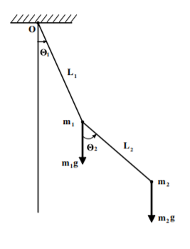
Consider the double pendulum comprising masses
$m_{1}$
and
$m_{2}$
connected by inextensible strings as shown in the figure. Assume that the motion of the pendulum takes place in a vertical plane.
1. Are there any equations of constraint? If so, what are they?
2. Find Lagrange’s equations for this system.
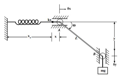
Consider the system shown in the figure which consists of a mass
$m$
suspended via a constrained massless link of length
$L$
where the point
$A$
is acted upon by a spring of spring constant
$k$
. The spring is unstretched when the massless link is horizontal. Assume that the holonomic constraints at
$A$
and
$B$
are frictionless.
1. Derive the equations of motion for the system using the method of Lagrange multipliers.
Consider a pendulum, with mass
$m$
, connected to a (horizontally) moveable support of mass
$M$
.
1. Determine the Lagrangian of the system.
2. Determine the equations of motion for $\theta \ll 1$ .
3. Find an equation of motion in $\theta$ alone. What is the frequency of oscillation?
4. What is the frequency of oscillation for $M\gg m$ ? Does this make sense?
A sphere of radius $\rho$ is constrained to roll without slipping on the lower half of the inner surface of a hollow cylinder of radius $R.$ Determine the Lagrangian function, the equation of constraint, and the Lagrange equations of motion. Find the frequency of small oscillations.
A particle moves in a plane under the influence of a force $f = −Ar^{\alpha - 1}$ directed toward the origin; $A$ and $\alpha (> 0)$ are constants. Choose generalized coordinates with the potential energy zero at the origin.
1. Find the Lagrangian equations of motion.
2. Is the angular momentum about the origin conserved?
3. Is the total energy conserved?
Two blocks, each of mass $M$ , are connected by an extensionless, uniform string of length $l$ . One block is placed on a frictionless horizontal surface, and the other block hangs over the side, the string passing over a frictionless pulley. Describe the motion of the system:
1. when the mass of the string is negligible
2. when the string has mass $m$ .
Two masses $m_{1}$ and $m_{2}$ $(m_{1}\neq m_{2})$ are connected by a rigid rod of length $d$ and of negligible mass. An extensionless string of length $l_{1}$ is attached to $m_{1}$ and connected to a fixed point of the support $P$ . Similarly a string of length $l_{2}$ $(l_{1}\neq l_{2})$ connects $m_{2}$ and $P$ . Obtain the equation of motion describing the motion in the plane of $m_{1},m_{2},$ and $P$ , and find the frequency of small oscillation around the equilibrium position.
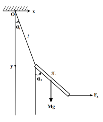
A thin uniform rigid rod of length $2L$ and mass $M$ is suspended by a massless string of length $l$ . Initially the system is hanging vertically downwards in the gravitational field $g$ . Use as generalized coordinates the angles given in the diagram.
1. Derive the Lagrangian for the system.
2. Use the Lagrangian to derive the equations of motion
3. A horizontal impulsive force $F_{x}$ in the $x$ direction strikes the bottom end of the rod for an infinitessimal time $\tau$ . Derive the initial conditions for the system immediately after the impulse has occurred.
4. Draw a diagram showing the geometry of the pendulum shortly after the impulse when the displacement angles are significant.

6.S: Lagrangian Dynamics (Summary)¶

Newtonian plausibility argument for Lagrangian mechanics¶

A justification for introducing the calculus of variations to classical mechanics becomes apparent when the concept of the Lagrangian $L\equiv T-U$ is used in the functional and time $t$ is the independent variable. It was shown that Newton’s equation of motion can be rewritten as

\frac{d}{dt}\frac{\partial L}{\partial \dot{q}_{i}}-\frac{\partial L}{ \partial q_{i}}=F_{q_{i}}^{EX} \tag{6.12}

where $F_{y_{i}}^{EX}$ are the excluded forces of constraint plus any other conservative or non-conservative forces not included in the potential $U.$ This corresponds to the Euler-Lagrange equation for determining the minimum of the time integral of the Lagrangian.

Equation 6.12 can be written as

\frac{d}{dt}\frac{\partial L}{\partial \dot{q}_{i}}-\frac{\partial L}{ \partial q_{i}}=\sum_{k}^{m}\lambda _{k}\left( t\right) \frac{\partial g_{k} }{\partial q_{i}}+F_{q_{i}}^{EXC}\tag{6.15}

where the Lagrange multiplier term accounts for holonomic constraint forces, and $F_{q_{i}}^{EXC}$ includes all additional forces not accounted for by the scalar potential $U$ , or the Lagrange multiplier terms $F_{q_{i}}^{HC}$ . The constraint forces can be included explicitly as generalized forces in the excluded term $F_{q_{i}}^{EXC}$ of Equation \text{(6.15)}.

d’Alembert’s Principle¶

It was shown that d’Alembert’s Principle

\sum_{i}^{N}(\mathbf{F}_{i}^{A}-\mathbf{\dot{p}}_{i})\cdot \delta \mathbf{r} _{i}=0 \tag{6.25}

cleverly transforms the principle of virtual work from the realm of statics to dynamics. Application of virtual work to statics primarily leads to algebraic equations between the forces, whereas d’Alembert’s principle applied to dynamics leads to differential equations.

Lagrange equations from d’Alembert’s Principle¶

After transforming to generalized coordinates, d’Alembert’s Principle leads to

\sum_{j}^{N} \left[ \left\{ \frac{d}{dt}\left( \frac{\partial T}{\partial \dot{q} _{j}}\right) -\frac{\partial T}{\partial q_{j}}\right\} -Q_{j}\right] \delta q_{j}=0\tag{6.38}

If all the $n$ coordinates $q_{j}$ are independent, then Equation \text{(6.38)} implies that the term in the square brackets is zero for each individual value of $j$ . That is, this implies the basic Euler-Lagrange equations of motion.

The handling of both conservative and non-conservative generalized forces $Q_j$ is best achieved by assuming that the generalized force $Q_j = \sum^n_i \mathbf{F}_i^A \cdot \frac{\partial \mathbf{\bar{r}}_i}{\partial q_j}$ can be partitioned into a conservative velocity-independent term, that can be expressed in terms of the gradient of a scalar potential, $-\nabla U_i$ , plus an excluded generalized force $Q^{EX}_j$ which contains the non-conservative, velocity-dependent, and all the constraint forces not explicitly included in the potential $U_j$ . That is,

Q_j = -\nabla U_j + Q_j^{EX} \tag{6.41}

Inserting \text{(6.41)} into \text{(6.38)}, and assuming that the potential $U$ is velocity independent, allows \text{(6.38)} to be rewritten as

\sum_{j} \left[ \left\{ \frac{d}{dt}\left( \frac{\partial (T - U)}{\partial \dot{q} _{j}}\right) -\frac{\partial (T - U)}{\partial q_{j}}\right\} -Q_{j}^{EX} \right] \delta q_{j}=0\tag{6.42}

Expressed in terms of the standard Lagrangian $L = T - U$ this gives

\sum_{j}^{N} \left[ \left\{ \frac{d}{dt}\left( \frac{\partial L}{\partial \dot{q} _{j}}\right) -\frac{\partial L}{\partial q_{j}}\right\} -Q_{j}^{EX} \right] \delta q_{j}=0\tag{6.44}

Note that Equation \text{(6.44)} contains the basic Euler-Lagrange Equation \text{(6.38)} for the special case when $U = 0$ . In addition, note that if all the generalized coordinates are independent, then the square bracket terms are zero for each value of $j$ , which leads to the $n$ general Euler-Lagrange equations of motion

\left\{ \frac{d}{dt}\left( \frac{\partial L}{\partial \dot{q} _{j}}\right) -\frac{\partial L}{\partial q_{j}}\right\} = Q_{j}^{EX} \tag{6.45}

where $n \geq j \geq 1$ . Newtonian mechanics has trouble handling constraint forces because they lead to coupling of the degrees of freedom. Lagrangian mechanics is more powerful since it provides the following three ways to handle such correlated motion.

1) Minimal set of generalized coordinates¶

If the $n$ coordinates $q_j$ are independent, then the square bracket equals zero for each value of $j$ in Equation \text{(6.44)}, which corresponds to Euler’s equation for each of the $n$ independent coordinates. If the $n$ generalized coordinates are coupled by $m$ constraints, then the coordinates can be transformed to a minimal set of $s = n − m$ independent coordinates which then can be solved by applying Equation \text{(6.45)} to the minimal set of $s$ independent coordinates.

2) Lagrange multipliers approach¶

The Lagrangian method concentrates solely on active forces, completely ignoring all other internal forces. In Lagrangian mechanics the generalized forces, corresponding to each generalized coordinate, can be partitioned three ways

Q_{j}=-\nabla U+\sum_{k=1}^{m}\lambda _{k}\frac{\partial g_{k}}{\partial q_{j}}(\mathbf{q},t)+Q_{j}^{EXC} \nonumber

where the velocity-independent conservative forces can be absorbed into a scalar potential $U$ , the holonomic constraint forces can be handled using the Lagrange multiplier term $\sum_{k=1}^{m}\lambda _{k}\frac{\partial g_{k} }{\partial q_{j}}(\mathbf{q},t)$ , and the remaining part of the active forces can be absorbed into the generalized force $Q_{j}^{EXC}$ . The scalar potential energy $U$ is handled by absorbing it into the standard Lagrangian $L=T-U$ . If the constraint forces are holonomic then these forces are easily and elegantly handled by use of Lagrange multipliers. All remaining forces, including dissipative forces, can be handled by including them explicitly in the generalized force $Q_{j}^{EXC}$ .

Combining the above two equations gives

\sum_{j}^{N}\left[ \left\{ \frac{d}{dt}\left( \frac{\partial L}{\partial \dot{q}_{j}}\right) -\frac{\partial L}{\partial q_{j}}\right\} -Q_{j}^{EXC}-\sum_{k=1}^{m}\lambda _{k}\frac{\partial g_{k}}{\partial q_{j}}( \mathbf{q},t)\right] \delta q_{j}=0 \tag{6.56}

Use of the Lagrange multipliers to handle the $m$ constraint forces ensures that all $n$ infinitessimals $\delta q_{j}$ are independent implying that the expression in the square bracket must be zero for each of the $n$ values of $j$ . This leads to $n$ Lagrange equations plus $m$ constraint relations

\left\{ \frac{d}{dt}\left( \frac{\partial L}{\partial \dot{q}_{j}}\right) - \frac{\partial L}{\partial q_{j}}\right\} =Q_{j}^{EXC}+\sum_{k=1}^{m}\lambda _{k}\frac{\partial g_{k}}{\partial q_{j}}(\mathbf{q},t) \tag{6.60}

where $j = 1,2,3, \dots n.$

3) Generalized forces approach¶

The two right-hand terms in \text{(6.60)} can be understood to be those forces acting on the system that are not absorbed into the scalar potential $U$ component of the Lagrangian $L$ . The Lagrange multiplier terms $\sum_{k=1}^{m}\lambda _{k}\frac{\partial g_{k}}{\partial q_{j}}(\mathbf{q},t)$ account for the holonomic forces of constraint that are not included in the conservative potential or in the generalized forces $Q_j^{EXC}$ . The generalized force

Q^{EXC}_j = \sum^{n}_i \mathbf{F}^A_i \cdot \frac{\partial \mathbf{r}_i}{\partial p_j} \tag{6.17}

is the sum of the components in the $q_j$ direction for all external forces that have not been taken into account by the scalar potential or the Lagrange multipliers. Thus the non-conservative generalized force $Q^{EXC}_j$ contains non-holonomic constraint forces, including dissipative forces such as drag or friction, that are not included in $U$ , or used in the Lagrange multiplier terms to account for the holonomic constraint forces.

Applying the Euler-Lagrange equations in mechanics:¶

The optimal way to exploit Lagrangian mechanics is as follows:

Select a set of independent generalized coordinates.
Partition the active forces into three groups:
1. Conservative one-body forces
2. Holonomic constraint forces
3. Generalized forces
Minimize the number of generalized coordinates.
Derive the Lagrangian
Derive the equations of motion

Velocity-dependent Lorentz force:¶

Usually velocity-dependent forces are non-holonomic. However, electromagnetism is a special case where the velocity-dependent Lorentz force $\mathbf{F}=q(\mathbf{E}+\mathbf{v\times B})$ can be obtained from a velocity-dependent potential function $U(q,\overset{.}{q},t)$ . It was shown that the velocity-dependent potential

U=q\Phi -q\mathbf{v}\cdot \mathbf{A} \tag{6.74}

leads to the Lorentz force where $\Phi$ is the scalar electric potential and $\mathbf{A}$ the vector potential.

Time-dependent forces:¶

It was shown that time-dependent forces can lead to complicated motion having both stable regions and unstable regions of motion that can exhibit chaos.

Impulsive forces:¶

A generalized impulse $\tilde{Q}_{j}$ can be derived for an instantaneous impulsive force from the time integral of the impulsive forces $\mathbf{P} _{i}$ given by equation $(3.12.49)$ using the time integral of equation $(7.2.13)$ , that is

\Delta p_{j}=\tilde{Q}_{j}=\lim_{\tau \rightarrow 0}\int_{t}^{t+\tau }Q_{j}^{EXC}d\tau \equiv \lim_{\tau \rightarrow 0}\int_{t}^{t+\tau }\sum_{i} \mathbf{F}_{i}^\cdot \frac{\partial \mathbf{r}_{i}}{\partial q_{j}}d\tau =\sum_{i}\mathbf{\tilde{P}}_{i}^\cdot \frac{\partial \mathbf{r}_{i}}{ \partial q_{j}} \tag{6.79}

Note that the generalized impulse $\tilde{Q}_{j}$ can be a translational impulse $\mathbf{\tilde{P}}_{j}$ with corresponding translational variable $q_{j}$ or an angular impulsive torque $\mathbf{\tilde{T}}_{j}$ with corresponding angular variable $\phi _{j}$ .

Comparison of Newtonian and Lagrangian mechanics:¶

In contrast to Newtonian mechanics, which is based on knowing all the vector forces acting on a system, Lagrangian mechanics can derive the equations of motion using generalized coordinates without requiring knowledge of the constraint forces acting on the system. Lagrangian mechanics provides a remarkably powerful, and incredibly consistent, approach to solving for the equations of motion in classical mechanics which is especially powerful for handling systems that are subject to holonomic constraints.

Footnotes¶

This proof, plus the notation, conform with that used by Goldstein [Go50] and by other texts on classical mechanics.
↩
This problem is solved in detail in example 3.19 of “Classical Mechanics and Relativity”. by Muller-Kirsten $\left[ Mu06\right]$ .
↩