7. Symmetries, Invariance and the Hamiltonian - Variational Principles in Classical Mechanics

7.1: Introduction to Symmetries, Invariance, and the Hamiltonian¶

The chapter 7 discussion of Lagrangian dynamics illustrates the power of Lagrangian mechanics for deriving the equations of motion. In contrast to Newtonian mechanics, which is expressed in terms of force vectors acting on a system, the Lagrangian method, based on d’Alembert’s Principle or Hamilton’s Principle, is expressed in terms of the scalar kinetic and potential energies of the system. The Lagrangian approach is a sophisticated alternative to Newton’s laws of motion, that provides a simpler derivation of the equations of motion that allows constraint forces to be ignored. In addition, the use of Lagrange multipliers or generalized forces allows the Lagrangian approach to determine the constraint forces when these forces are of interest. The equations of motion, derived either from Newton’s Laws or Lagrangian dynamics, can be non-trivial to solve mathematically. It is necessary to integrate second-order differential equations, which for $n$ degrees of freedom, imply $2n$ constants of integration.

Chapter 7 will explore the remarkable connection between symmetry and invariance of a system under transformation, and the related conservation laws that imply the existence of constants of motion. Even when the equations of motion cannot be solved easily, it is possible to derive important physical principles regarding the first-order integrals of motion of the system directly from the Lagrange equation, as well as for elucidating the underlying symmetries plus invariance. This property is contained in Noether’s theorem which states that conservation laws are associated with differentiable symmetries of a physical system.

7.2: Generalized Momentum¶

Consider a holonomic system of $N$ masses under the influence of conservative forces that depend on position $q_{j}$ but not velocity $\dot{q}_{j}$ , that is, the potential is velocity independent. Then for the $x$ coordinate of particle $i$ for $N$ particles

\begin{align} \frac{\partial L}{\partial \dot{x}_{i}} &= \frac{\partial T}{\partial \dot{x} _{i}}-\frac{\partial U}{\partial \dot{x}_{i}}=\frac{\partial T}{\partial \dot{x}_{i}} \tag{7.1} \\[4pt] &= \frac{\partial }{\partial \dot{x}_{i}}\sum_{i=1}^{N}\frac{1}{2} m_{i}\left( \dot{x}_{i}^{2}+\dot{y}_{i}^{2}+\dot{z}_{i}^{2}\right) \notag\\[4pt] &= m_{i}\dot{x}_{i}=p_{i,x} \notag\end{align}

Thus for a holonomic, conservative, velocity-independent potential we have

\frac{\partial L}{\partial \dot{x}_{i}}=p_{i,x} \tag{7.2}

which is the $x$ component of the linear momentum for the $i^{th}$ particle.

This result suggests an obvious extension of the concept of momentum to generalized coordinates. The generalized momentum associated with the coordinate $q_{j}$ is defined to be

\frac{\partial L}{\partial \dot{q}_{j}}\equiv p_{j}\tag{7.3}

Note that $p_{j}$ also is called the conjugate momentum orcanonical momentum to $q_{j}$ where $q_{j},p_{j}$ are conjugate, or canonical, variables. Remember that the linear momentum $p_{j}$ is the first-order time integral given by equation $(2.4.1)$ . If $q_{j}$ is not a spatial coordinate, then $p_{j}$ is the generalized momentum, not the kinematic linear momentum. For example, if $q_{j}$ is an angle, then $p_{j}$ will be angular momentum. That is, the generalized momentum may differ from the usual linear or angular momentum since the definition 7.3 is more general than the usual $p_{x}=m \dot{x}$ definition of linear momentum in classical mechanics. This is illustrated by the case of a moving charged particles $m_{j},e_{j}$ in an electromagnetic field. Chapter 6 showed that electromagnetic forces on a charge $e_{j}$ can be described in terms of a scalar potential $U_{j}$ where

U_{j}=e_{j}(\Phi -\mathbf{A\cdot v}_{j}\mathbf{)}\tag{7.4}

Thus the Lagrangian for the electromagnetic force can be written as

L=\sum_{j=1}^{N}\left[ \frac{1}{2}m_{j}\mathbf{v}_{j}\cdot \mathbf{v} _{j}-e_{j}(\Phi -\mathbf{A\cdot v}_{j}\mathbf{)}\right]\tag{7.5}

The generalized momentum to the coordinate $x_{j}$ for charge $e_{j},$ and mass $m_{j},$ is given by the above Lagrangian

p_{j,x}=\frac{\partial L}{\partial \dot{x}_{j}}=m_{j}\dot{x}_{j}+e_{j}A_{x}\tag{7.6}

Note that this includes both the mechanical linear momentum plus the correct electromagnetic momentum. The fact that the electromagnetic field carries momentum should not be a surprise since electromagnetic waves also carry energy as is illustrated by the transmission of radiant energy from the sun.

Example 7.2.1: Feynman’s angular-momentum paradox

Feynman posed the following paradox [Fey84]. A circular insulating disk $,$ mounted on frictionless bearings, has a circular ring of total charge $q$ uniformly distributed around the perimeter of the circular disk at the radius $R$ . A superconducting long solenoid of radius $s$ , where $s<R$ , is fixed to the disk and is mounted coaxial with the bearings. The moment of inertia of the system about the rotation axis is $I$ . Initially the disk plus superconducting solenoid are stationary with a steady current producing a uniform magnetic field $B_{0}$ inside the solenoid. Assume that a rise in temperature of the solenoid destroys the superconductivity leading to a rapid dissipation of the electric current and resultant magnetic field. Assume that the system is free to rotate, no other forces or torques are acting on the system, and that the charge carriers in the solenoid have zero mass and thus do not contribute to the angular momentum. Does the system rotate when the current in the solenoid stops?

Initially the system is stationary with zero mechanical angular momentum. Faraday’s Law states that, when the magnetic field dissipates from $B_{0}$ to zero, there will be a torque $\mathbf{N}$ acting on the circumferential charge $q$ at radius $R$ due to the change in magnetic flux $\Phi$ .

\mathbf{N}(t)=-qR\frac{d\Phi }{dt} \nonumber

Since $\frac{d\Phi }{dt}<0$ , this torque leads to an angular impulse which will equal the final mechanical angular momentum.

\mathbf{L}_{final}^{MECH}=\mathbf{T=}\int_{t}\mathbf{N}(t)dt=qR\mathbf{\Phi }\nonumber

The initial angular momentum in the electromagnetic field can be derived using Equation 7.6, plus Stoke’s theorem (Appendix 19.8.3) . Equation 2.12.56 gives that the final angular momentum equals the angular impulse

\mathbf{L}_{initial}^{EM}=R\int_{t}\oint r\dot{p}_{\phi }dldt=R\oint rp_{\phi }dl=qR\oint A_{\phi }dl=qR\int \mathbf{B\cdot dS=}qR\mathbf{\Phi }\nonumber

where $\Phi =\oint A_{\phi }dl=\int \mathbf{B\cdot dS}$ is the initial total magnetic flux through the solenoid. Thus the total initial angular momentum is given by

\mathbf{L}_{initial}^{TOTAL}=0+\mathbf{L}_{initial}^{EM}=qR\mathbf{\Phi }\nonumber

Since the final electromagnetic field is zero the final total angular momentum is given by

\mathbf{L}_{final}^{TOTAL}=\mathbf{L}_{final}^{MECH}+0=qR\mathbf{\Phi }\nonumber

Note that the total angular momentum is conserved. That is, initially all the angular momentum is stored in the electromagnetic field, whereas the final angular momentum is all mechanical. This explains the paradox that the mechanical angular momentum is not conserved, only the total angular momentum of the system is conserved, that is, the sum of the mechanical and electromagnetic angular momenta.

7.3: Invariant Transformations and Noether’s Theorem¶

One of the great advantages of Lagrangian mechanics is the freedom it allows in choice of generalized coordinates which can simplify derivation of the equations of motion. For example, for any set of coordinates, $q_{j},$ a reversible point transformation can define another set of coordinates $q_{j}^{\prime }$ such that

q_{j}^{\prime }=q_{j}^{\prime }(q_{1},q_{2},..q_{n};t)

The new set of generalized coordinates satisfies Lagrange’s equations of motion with the new Lagrangian

L(q^{\prime },\dot{q}^{\prime },t)=L(q,\dot{q},t)

The Lagrangian is a scalar, with units of energy, which does not change if the coordinate representation is changed. Thus $L(q^{\prime },\dot{q} ^{\prime },t)$ can be derived from $L(q,\dot{q},t)$ by substituting the inverse relation $q_{i}=q_{i}(q_{1}^{\prime },q_{2}^{\prime },..q_{n}^{\prime };t)$ into $L(q,\dot{q},t).$ That is, the value of the Lagrangian $L$ is independent of which coordinate representation is used. Although the general form of Lagrange’s equations of motion is preserved in any point transformation, the explicit equations of motion for the new variables usually look different from those with the old variables. A typical example is the transformation from cartesian to spherical coordinates. For a given system, there can be particular transformations for which the explicit equations of motion are the same for both the old and new variables. Transformations for which the equations of motion are invariant, are called invariant transformations. It will be shown that if the Lagrangian does not explicitly contain a particular coordinate of displacement $q_{i},$ then the corresponding conjugate momentum, $p_{i},$ is conserved. This relation is called Noether’s theorem which states “For each symmetry of the Lagrangian, there is a conserved quantity".

Noether’s Theorem will be used to consider invariant transformations for two dependent variables, $x(t),$ and $\theta (t),$ plus their conjugate momenta $p_{x}$ and $p_{\theta }$ . For a closed system, these provide up to six possible conservation laws for the three axes. Then we will discuss the independent variable $t,$ and its relation to the Generalized Energy Theorem, which provides another possible conservation law. For simplicity, these discussions will assume that the systems are holonomic and conservative.

The Lagrange equations using generalized coordinates for holonomic systems, was given by equation $(6.5.12)$ to be

\left\{ \frac{d}{dt}\left( \frac{\partial L}{\partial \dot{q}_{j}}\right) -\frac{ \partial L}{\partial q_{j}}\right\} =\sum_{k=1}^{m}\lambda _{k}\frac{ \partial g_{k}}{\partial q_{j}}(\mathbf{q},t)+Q_{j}^{EXC}

This can be written in terms of the generalized momentum as

\left\{ \frac{d}{dt}p_{j}-\frac{\partial L}{\partial q_{j}}\right\} =\sum_{k=1}^{m}\lambda _{k}\frac{\partial g_{k}}{\partial q_{j}}(\mathbf{q} ,t)+Q_{j}^{EXC}

or equivalently as

\dot{p}_{j}=\frac{\partial L}{\partial q_{j}}+\left[ \sum_{k=1}^{m}\lambda _{k}\frac{\partial g_{k}}{\partial q_{j}}(\mathbf{q},t)+Q_{j}^{EXC}\right]

Note that if the Lagrangian $L$ does not contain $q_{i}$ explicitly, that is, the Lagrangian is invariant to a linear translation, or equivalently, is spatially homogeneous, and if the Lagrange multiplier constraint force and generalized force terms are zero, then

\frac{\partial L}{\partial q_{j}}+\left[ \sum_{k=1}^{m}\lambda _{k}\frac{ \partial g_{k}}{\partial q_{j}}(\mathbf{q},t)+Q_{j}^{EXC}\right] =0

In this case the Lagrange equation reduces to

\dot{p}_{j}=\frac{dp_{j}}{dt}=0 \tag{7.13}

Equation 7.13 corresponds to $p_{j}$ being a constant of motion. Stated in words, the generalized momentum $p_{i}$ is a constant of motion if the Lagrangian is invariant to a spatial translation of $q_{i}$ , and the constraint plus generalized force terms are zero. Expressed another way, if the Lagrangian does not contain a given coordinate $q_{i}$ and the corresponding constraint plus generalized forces are zero, then the generalized momentum associated with this coordinate is conserved. Note that this example of Noether’s theorem applies to any component of $\mathbf{q}$ . For example, in the uniform gravitational field at the surface of the earth, the Lagrangian does not depend on the $x$ and $y$ coordinates in the horizontal plane, thus $p_{x}$ and $p_{y}$ are conserved, whereas, due to the gravitational force, the Lagrangian does depend on the vertical $z$ axis and thus $p_{z}$ is not conserved.

Example 7.3.1: Atwoods machine

Assume that the linear momentum is conserved for the Atwood’s machine shown in the figure below.

Figure 7.3.1:Example of an Atwood’s machine

Let the left mass rise a distance $x$ and the right mass rise a distance $y$ . Then the middle mass must drop by $x+y$ to conserve the length of the string. The Lagrangian of the system is

L= \frac{1}{2}(4m)\dot{x}^{2}+\frac{1}{2}(3m)(-\dot{x}-\dot{y})^{2}+\frac{1}{2}m \dot{y}^{2}-\left( 4mgx+3mg(-x-y)+mgy\right) =\frac{7}{2}m\dot{x}^{2}+3m\dot{ x}\dot{y}+2m\dot{y}^{2}-mg(x-2y) \nonumber

Note that the transformation

\begin{align*} x &= x_{0}+2\epsilon \\[4pt] y &=y_{0}+\epsilon\end{align*}

results in the potential energy term $mg(x-2y)=mg(x_{0}-2y_{0})$ which is a constant of motion. As a result the Lagrangian is independent of $\epsilon ,$ which means that it is invariant to the small perturbation $\epsilon ,$ and thus $\frac{dL}{d\epsilon }=0.$ Therefore, according to Noether’s theorem, the corresponding linear momentum $P_{\epsilon }=\frac{dL}{d\dot{\epsilon}}$ is conserved. This conserved linear momentum then is given by

\begin{align*} P_{\epsilon } &=\frac{dL}{d\dot{\epsilon}}=\frac{\partial L}{\partial \dot{x}} \frac{\partial \dot{x}}{\partial \dot{\epsilon}}+\frac{\partial L}{\partial \dot{y}}\frac{\partial \dot{y}}{\partial \dot{\epsilon}} \\[4pt] &=m(7\dot{x}+3\dot{y} )(2)+m(3\dot{x}+4\dot{y})=m(17\dot{x}+10\dot{y}) \end{align*}

Thus, if the system starts at rest with $P_{\epsilon }=0$ , then $\dot{x}$ always equals $-\frac{10}{17}\dot{y}$ since $P_{\epsilon }$ is constant.

Note that this also can be shown using the Euler-Lagrange equations in that $\Lambda _{x}L=0$ and $\Lambda _{y}L=0$ give

\begin{aligned} 7m\ddot{x}+3m\ddot{y} &=&-mg \\ 3m\ddot{x}+4m\ddot{y} &=&2mg\end{aligned}

Adding the second equation to twice the first gives

17m\ddot{x}+10m\ddot{y}=\frac{d}{dt}(17m\dot{x}+10m\dot{y})=0 \nonumber

This is the result obtained directly using Noether’s theorem.

7.4: Rotational invariance and conservation of angular momentum¶

The arguments, used above, apply equally well to conjugate momenta $p_{\theta }$ and $\theta$ for rotation about any axis. The Lagrange equation is

\left\{ \frac{d}{dt}p_{\theta }-\frac{\partial L}{\partial \theta }\right\} =\sum_{k=1}^{m}\lambda _{k}\frac{\partial g_{k}}{\partial \theta }(\mathbf{q} ,t)+Q_{\theta }^{EXC} \tag{7.14}

If no constraint or generalized torques act on the system, then the right-hand side of Equation 7.14 is zero. Moreover if the Lagrangian in not an explicit function of $\theta ,$ then $\frac{\partial L}{\partial \theta }=0,$ and assuming that the constraint plus generalized torques are zero, then $p_{\theta }$ is a constant of motion.

Noether’s Theorem illustrates this general result which can be stated as, if the Lagrangian is rotationally invariant about some axis, then the component of the angular momentum along that axis is conserved. Also this is true for the more general case where the Lagrangian is invariant to rotation about any axis, which leads to conservation of the total angular momentum.

Example 7.4.1: Conservation of angular momentum for rotational invariance

Figure 7.4.1:Infinitessimal rotation

The Noether theorem result for rotational-invariance about an axis also can be derived using cartesian coordinates as shown below. As discussed in appendix 19.4, it is necessary to limit discussion of rotation to infinitessimal rotation angles in order to represent the rotation by a vector. Consider an infinitessimal rotation $\delta \theta$ about some axis, which is a vector. As illustrated in the adjacent figure, this can be expressed as

\delta \mathbf{r}=\delta \mathbf{\theta }\times \mathbf{r} \nonumber

The velocity vectors also change on rotation of the system obeying the transformation equation which is common to all vectors, that is,

\delta \mathbf{\dot{r}}=\delta \mathbf{\theta }\times \mathbf{\dot{r}}\nonumber

If the Lagrangian is unaffected by the orientation of the system, that is, it is rotationally invariant, then it can be shown that the angular momentum is conserved. For example, consider that the Lagrangian is invariant to rotation about some axis $q_{i}$ . Since the Lagrangian is a function

L=L(q_{i},\dot{q}_{i};t)\nonumber

then the expression that the Lagrangian does not change due to an infinitesimal rotation $\delta \theta$ about this axis can be expressed as

\delta L=\sum_{i}\frac{\partial L}{\partial x_{i}}\delta x_{i}+\sum_{i}\frac{ \partial L}{\partial \dot{x}_{i}}\delta \dot{x}_{i}=0 \tag{$A$}

where cartesian coordinates have been used.

Using the generalized momentum

\frac{\partial L}{\partial \dot{x}_{i}}=p_{i}\nonumber

then, Lagrange’s equation gives

\frac{d}{dt}p_{i}-\frac{\partial L}{\partial x_{i}}=0\nonumber

that is

\dot{p}_{i}=\frac{\partial L}{\partial x_{i}}\nonumber

Inserting this into Equation a1 gives

\delta L=\sum_{i}^{3}\dot{p}\delta x_{i}+\sum_{i}^{3}p_{i}\delta \dot{x} _{i}=0\nonumber

This is equivalent to the scalar products

\mathbf{\dot{p}}\cdot \delta \mathbf{r}+\mathbf{p}\cdot \delta \mathbf{\dot{r }}=0\nonumber

For an infinitessimal rotation $\delta \theta ,$ then $\delta r=\delta \theta \times r\,$ and $\delta \dot{r}=\delta \theta \times \dot{r}$ . Therefore

\mathbf{\dot{p}}\cdot \left( \delta \mathbf{\theta }\times \mathbf{r}\right) +\mathbf{p}\cdot \left( \delta \mathbf{\theta }\times \mathbf{\dot{r}} \right) =0\nonumber

The cyclic order can be permuted giving

\begin{aligned} \delta \mathbf{\theta }\cdot \left( \mathbf{r}\times \mathbf{\dot{p}}\right) +\delta \mathbf{\theta }\cdot \left( \mathbf{\dot{r}}\times \mathbf{p} \right) &=&0 \\ \delta \mathbf{\theta }\cdot \left[ \left( \mathbf{r}\times \mathbf{\dot{p}} \right) +\left( \mathbf{\dot{r}}\times \mathbf{p}\right) \right] &=&0 \\ \delta \mathbf{\theta }\cdot \frac{d}{dt}\left( \mathbf{r}\times \mathbf{p} \right) &=&0\end{aligned}

Because the infinitessimal angle $\delta \theta$ is arbitrary, then the time derivative

\frac{d}{dt}\left( \mathbf{r}\times \mathbf{p}\right) =0\nonumber

about the axis of rotation $\delta \theta .$ But the bracket $\left( \mathbf{r}\times \mathbf{p}\right)$ equals the angular momentum. That is;

\text{Angular momentum = }\left( \mathbf{r}\times \mathbf{p}\right) =\text{ constant}\nonumber

This proves the Noether’ theorem that the angular momentum about any axis is conserved if the Lagrangian is rotationally invariant about that axis

Example 7.4.1: Diatomic molecules and axially-symmetric nuclei

An interesting example of Noether’s theorem applies to diatomic molecules such as $H_{2},N_{2},F_{2},O_{2},Cl_{2}$ and $Br_{2}$ . The electric field produced by the two charged nuclei of the diatomic molecule has cylindrical symmetry about the axis through the two nuclei. Electrons are bound to this dumbbell arrangement of the two nuclear charges which may be rotating and vibrating in free space. Assuming that there are no external torques acting on the diatomic molecule in free space, then the angular momentum about any fixed axis in free space must be conserved according to Noether’s theorem. If no external torques are applied, then the component of the angular momentum about any fixed axis is conserved, that is, the total angular momentum is conserved. What is especially interesting is that since the electrostatic potential, and thus the Lagrangian, of the diatomic molecule has cylindrical symmetry, that is $\frac{\partial L}{\partial \phi }=0$ , then the component of the angular momentum with respect to this symmetry axis also is conserved irrespective of how the diatomic molecule rotates or vibrates in free space. That is, an additional symmetry has been identified that leads to an additional conservation law that applies to the angular momentum.

An example of Noether’s theorem is in nuclear physics where some nuclei have a spheroidal shape similar to an american football or a rugby ball. This spheroidal shape has an axis of symmetry along the long axis. The Lagrangian is rotationally invariant about the symmetry axis resulting in the angular momentum about the symmetry axis being conserved in addition to conservation of the total angular momentum.

7.5: Cyclic Coordinates¶

Translational and rotational invariance occurs when a system has a cyclic coordinate $q_{k}.$ A cyclic coordinate is one that does not explicitly appear in the Lagrangian. The term cyclic is a natural name when one has cylindrical or spherical symmetry. In Hamiltonian mechanics a cyclic coordinate often is called an ignorable coordinate . By virtue of Lagrange’s equations

\frac{d}{dt}\frac{\partial L}{\partial \dot{q}_{k}}-\frac{\partial L}{ \partial q_{k}}=0

then a cyclic coordinate $q_{k},$ is one for which $\frac{\partial L}{ \partial q_{k}}=0$ . Thus

\frac{d}{dt}\frac{\partial L}{\partial \dot{q}_{k}}=\dot{p}_{k}=0

that is, $\ p_{k}$ is a constant of motion if the conjugate coordinate $q_{k}$ is cyclic. This is just Noether’s Theorem.

7.6: Kinetic Energy in Generalized Coordinates¶

Application of Noether’s theorem to the conservation of energy requires the kinetic energy to be expressed in generalized coordinates. In terms of fixed rectangular coordinates, the kinetic energy for $N$ bodies, each having three degrees of freedom, is expressed as

T=\frac{1}{2}\sum_{\alpha =1}^{N}\sum_{i=1}^{3}m_{\alpha }\dot{x}_{\alpha ,i}^{2}\tag{7.17}

These can be expressed in terms of generalized coordinates as $x_{\alpha ,i}=x_{\alpha ,i}(q_{j},t)$ and in terms of generalized velocities

\dot{x}_{\alpha ,i}=\sum_{j=1}^{s}\frac{\partial x_{\alpha ,i}}{\partial q_{j}}\dot{q}_{j}+\frac{\partial x_{\alpha ,i}}{\partial t}

Taking the square of $\dot{x}_{\alpha ,i}$ and inserting into the kinetic energy relation gives

T(\mathbf{q},\mathbf{\dot{q}},t)=\sum_{\alpha }\sum_{i,j,k}\frac{1}{2} m_{\alpha }\frac{\partial x_{\alpha ,i}}{\partial q_{j}}\frac{\partial x_{\alpha ,i}}{\partial q_{k}}\dot{q}_{j}\dot{q}_{k}+\sum_{\alpha }\sum_{i,j}m_{\alpha }\frac{\partial x_{\alpha ,i}}{\partial q_{j}}\frac{ \partial x_{\alpha ,i}}{\partial t}\dot{q}_{j}+\sum_{\alpha }\sum_{i}\frac{1 }{2}m_{\alpha }\left( \frac{\partial x_{\alpha ,i}}{\partial t}\right) ^{2}

This can be abbreviated as

T(\mathbf{q},\mathbf{\dot{q}},t)=T_{2}(\mathbf{q},\mathbf{\dot{q}},t)+T_{1}( \mathbf{q},\mathbf{\dot{q}},t)+T_{0}(\mathbf{q},t)

where

\begin{align} \tag{7.21} T_{2}(\mathbf{q},\mathbf{\dot{q}},t) &=&\sum_{\alpha }\sum_{i,j,k}\frac{1}{2} m_{\alpha }\frac{\partial x_{\alpha ,i}}{\partial q_{j}}\frac{\partial x_{\alpha ,i}}{\partial q_{k}}\dot{q}_{j}\dot{q}_{k}=\sum_{j,k}a_{jk}\dot{q} _{j}\dot{q}_{k} \\ T_{1}(\mathbf{q},\mathbf{\dot{q}},t) &=&\sum_{\alpha }\sum_{i,j}m_{\alpha } \frac{\partial x_{\alpha ,i}}{\partial q_{j}}\frac{\partial x_{\alpha ,i}}{ \partial t}\dot{q}_{j}=\sum_{j,k}b_{j}\dot{q}_{j} \\ T_{0}(\mathbf{q},t) &=&\sum_{\alpha }\sum_{i}\frac{1}{2}m_{\alpha }\left( \frac{\partial x_{\alpha ,i}}{\partial t}\right) ^{2}\end{align}

where

a_{jk}\equiv \sum_{\alpha =1}^{n}\sum_{i,=1}^{3}\frac{1}{2}m_{\alpha }\frac{ \partial x_{\alpha ,i}}{\partial q_{j}}\frac{\partial x_{\alpha ,i}}{ \partial q_{k}}

When the transformed system is scleronomic, time does not appear explicitly in the transformation equations to generalized coordinates since** $\frac{\partial x_{\alpha ,i}}{\partial t}=0$ . Then $T_{1}=T_{0}=0$ , and the kinetic energy reduces to a homogeneous quadratic function of the generalized velocities

T(\mathbf{q},\mathbf{ \dot{q}},t)=T_{2}(\mathbf{q},\mathbf{\dot{q}},t) \tag{7.25}

A useful relation can be derived by taking the differential of Equation 7.21 with respect to $\dot{q}_{l}$ . That is

\frac{\partial T_{2}(\mathbf{q},\mathbf{\dot{q}},t)}{\partial \dot{q}_{l}} =\sum_{k}a_{lk}\dot{q}_{k}+\sum_{j}a_{jl}\dot{q}_{j}

Multiply this by $\dot{q}_{l}$ and sum over $l$ gives

\sum_{l}\dot{q}_{l}\frac{\partial T_{2}(\mathbf{q},\mathbf{\dot{q}},t)}{ \partial \dot{q}_{l}}=\sum_{k,l}a_{lk}\dot{q}_{k}\dot{q}_{l}+\sum_{j,l}a_{jl} \dot{q}_{j}\dot{q}_{l}=2\sum_{j,k}a_{lk}\dot{q}_{k}\dot{q}_{l}=2T_{2}

Similarly, the products of the generalized velocities $\dot{q},$ with the corresponding derivatives of $T_{1}$ and $T_{0}$ give $$

\begin{align} \tag{7.27} \sum_{l}\dot{q}_{l}\frac{\partial T_{2}}{\partial \dot{q}_{l}} &=&2T_{2} \\ \sum_{l}\dot{q}_{l}\frac{\partial T_{1}(\mathbf{q},\mathbf{\dot{q}},t)}{ \partial \dot{q}_{l}} &=&T_{1}(\mathbf{q},\mathbf{\dot{q}},t) \\ \sum_{l}\dot{q}_{l}\frac{\partial T_{0}(\mathbf{q},t)}{\partial \dot{q}_{l}} &=&0\end{align}

Equation 7.25 gives that $T=T_{2}$ when the transformed system is scleronomic, i.e. $\frac{\partial x_{\alpha ,i}}{\partial t}=0,$ and then the kinetic energy is a quadratic function of the generalized velocities $\dot{q}_{j}$ . Using the definition of the generalized momentum equation $(7.2.3)$ , assuming $T=T_{2}$ , and that the potential $U$ is velocity independent, gives that

p_{l}\equiv \frac{\partial L}{\partial \dot{q}_{l}}=\frac{\partial T}{\partial \dot{q} _{l}}-\frac{\partial U}{\partial \dot{q}_{l}}=\frac{\partial T_{2}}{\partial \dot{q}_{l}}

Then Equation 7.27 reduces to the useful relation that

T_{2}=\frac{1}{2}\sum_{l}\dot{q}_{l}p_{l}=\frac{1}{2}\mathbf{\dot{q}\cdot p}

where, for compactness, the summation is abbreviated as a scalar product.

7.7: Generalized Energy and the Hamiltonian Function¶

Consider the time derivative of the Lagrangian, plus the fact that time is the independent variable in the Lagrangian. Then the total time derivative is

\frac{dL}{dt}=\sum_{j}\frac{\partial L}{\partial q_{j}}\dot{q}_{j}+\sum_{j} \frac{\partial L}{\partial \dot{q}_{j}}\ddot{q}_{j}+\frac{\partial L}{ \partial t} \tag{7.32}

The Lagrange equations for a conservative force are given by equation $(6.5.12)$ to be

\frac{d}{dt}\frac{\partial L}{\partial \dot{q}_{j}}-\frac{\partial L}{ \partial q_{j}}=Q_{j}^{EXC}+\sum_{k=1}^{m}\lambda _{k}\frac{\partial g_{k}}{ \partial q_{j}}(\mathbf{q},t) \tag{7.33}

The holonomic constraints can be accounted for using the Lagrange multiplier terms while the generalized force $Q_{j}^{EXC}$ includes non-holonomic forces or other forces not included in the potential energy term of the Lagrangian, or holonomic forces not accounted for by the Lagrange multiplier terms.

Substituting Equation 7.33 into Equation 7.32 gives

\begin{align} \frac{dL}{dt} &=&\sum_{j}\dot{q}_{j}\frac{d}{dt}\frac{\partial L}{\partial \dot{q}_{j}}-\sum_{j}\dot{q}_{j}\left[ Q_{j}^{EXC}+\sum_{k=1}^{m}\lambda _{k} \frac{\partial g_{k}}{\partial q_{j}}(\mathbf{q},t)\right] +\sum_{j}\frac{ \partial L}{\partial \dot{q}_{j}}\ddot{q}_{j}+\frac{\partial L}{\partial t} \notag \\ &=&\sum_{j}\frac{d}{dt}\left( \dot{q}_{j}\frac{\partial L}{\partial \dot{q} _{j}}\right) -\sum_{j}\dot{q}_{j}\left[ Q_{j}^{EXC}+\sum_{k=1}^{m}\lambda _{k}\frac{\partial g_{k}}{\partial q_{j}}(\mathbf{q},t)\right] +\frac{ \partial L}{\partial t}\end{align}

This can be written in the form

\frac{d}{dt}\left[ \sum_{j}\left( \dot{q}_{j}\frac{\partial L}{\partial \dot{ q}_{j}}\right) -L\right] =\sum_{j}\dot{q}_{j}\left[ Q_{j}^{EXC}+ \sum_{k=1}^{m}\lambda _{k}\frac{\partial g_{k}}{\partial q_{j}}(\mathbf{q},t) \right] -\frac{\partial L}{\partial t}

Define Jacobi’s Generalized Energy^[1]** $h(\mathbf{q},\mathbf{ \dot{q}},t)$ by

h(\mathbf{q},\mathbf{ \dot{q}},t)\equiv \sum_{j}\left( \dot{q}_{j}\frac{\partial L}{\partial \dot{q }_{j}}\right) -L(\mathbf{q},\mathbf{\dot{q}},t)

Jacobi’s generalized momentum, equation $7.2.3,$ can be used to express the generalized energy $h(q,\dot{q},t)$ in terms of the canonical coordinates $\dot{q}_{i}$ and $p_{i}$ , plus time $t$ . Define the Hamiltonian function to equal the generalized energy expressed in terms of the conjugate variables $(q_{j},p_{j})$ , that is,

H\left( \mathbf{q,p,}t\right) \equiv h(\mathbf{q},\mathbf{\dot{q}},t)\equiv \sum_{j}\left( \dot{q}_{j}\frac{\partial L}{\partial \dot{q}_{j}}\right) -L( \mathbf{q},\mathbf{\dot{q}},t)=\sum_{j}\left( \dot{q}_{j}p_{j}\right) -L( \mathbf{q},\mathbf{\dot{q}},t)

This Hamiltonian $H\left( \mathbf{q,p,}t\right)$ underlies Hamiltonian mechanics which plays a profoundly important role in most branches of physics as illustrated in chapters $8,15$ and 18.

7.8: Generalized energy theorem¶

The Hamilton function, $(7.7.6)$ plus equation $(7.7.4)$ lead to the generalized energy theorem

\frac{dH\left( \mathbf{q,p,}t\right) }{dt}=\frac{dh(\mathbf{q},\mathbf{\dot{q }},t)}{dt}=\sum_{j}\dot{q}_{j}\left[ Q_{j}^{EXC}+\sum_{k=1}^{m}\lambda _{k} \frac{\partial g_{k}}{\partial q_{j}}(\mathbf{q},t)\right] -\frac{\partial L( \mathbf{q},\mathbf{\dot{q}},t)}{\partial t}

Note that for the special case where all the external forces $\left[ Q_{j}^{EXC}+\sum_{k=1}^{m}\lambda _{k}\frac{\partial g_{k}}{\partial q_{j}}( \mathbf{q},t)\right] =0$ , then

\frac{dH}{dt}=-\frac{\partial L}{\partial t}

Thus the Hamiltonian is time independent if both** $\left[ Q_{j}^{EXC}+\sum_{k=1}^{m}\lambda _{k}\frac{\partial g_{k}}{\partial q_{j}}( \mathbf{q},t)\right] =0$ **and the Lagrangian are time-independent. For an isolated closed system having no external forces acting, then the Lagrangian is time independent because the velocities are constant, and there is no external potential energy. That is, the Lagrangian is time-independent, and

\frac{d}{dt}\left[ \sum_{j}\left( \dot{q}_{j}\frac{\partial L}{\partial \dot{ q}_{j}}\right) -L\right] =\frac{dH}{dt}=-\frac{\partial L}{\partial t}=0

As a consequence, the Hamiltonian $H\left( \mathbf{q,p,}t\right) ,$ and generalized energy $h(\mathbf{q},\mathbf{\dot{q}},t)$ , both are constants of motion if the Lagrangian is a constant of motion, and if the external non-potential forces are zero. This is an example of Noether’s theorem, where the symmetry of time independence leads to conservation of the conjugate variable, which is the Hamiltonian or Generalized energy.

7.9: Generalized energy and total energy¶

The generalized kinetic energy, equation $(7.6.4)$ , can be used to write the generalized Lagrangian as

L(\mathbf{q},\mathbf{ \dot{q}},t)=T_{2}(\mathbf{q},\mathbf{\dot{q}},t)+T_{1}(\mathbf{q},\mathbf{ \dot{q}},t)+T_{0}(\mathbf{q},t)-U(\mathbf{q},t)

If the potential energy $U$ does not depend explicitly on velocities $\dot{q }_{i}$ or time, then

\tag{7.42} p_{j}=\frac{\partial L}{\partial \dot{q}_{j}}=\frac{\partial \left( T-U\right) }{\partial \dot{q}_{j}}=\frac{\partial T}{\partial \dot{q}_{j}}

Equation 7.42 can be used to write the Hamiltonian, equation $(7.7.6)$ , as

H\left( \mathbf{q,p,}t\right) =\sum_{i}\left( \dot{q}_{j}\frac{\partial T_{2} }{\partial \dot{q}_{j}}\right) +\sum_{i}\left( \dot{q}_{j}\frac{\partial T_{1}}{\partial \dot{q}_{j}}\right) +\sum_{i}\left( \dot{q}_{j}\frac{ \partial T_{0}}{\partial \dot{q}_{j}}\right) -L(\mathbf{q},\mathbf{\dot{q}} ,t)

Using equations $(7.6.12)$ , $(7.6.13)$ , $(7.6.14)$ gives that the total generalized Hamiltonian $H\left( \mathbf{q,p,}t\right)$ equals

H\left( \mathbf{q,p,}t\right) =2T_{2}+T_{1}-(T_{2}+T_{1}+T_{0}-U)=T_{2}-T_{0}+U \tag{7.44}

But the sum of the kinetic and potential energies equals the total energy. Thus Equation 7.44 can be rewritten in the form

H\left( \mathbf{q,p,}t\right) =(T+U)-(T_{1}+2T_{0})=E-(T_{1}+2T_{0})

Note that Jacobi’s generalized energy and the Hamiltonian do not equal the total energy $E$ . However, in the special case where the transformation is scleronomic, then $T_{1}=T_{0}=0,$ and if the potential energy $U$ does not depend explicitly of $\dot{q}_{i}$ , then the**generalized energy (Hamiltonian) equals the total energy,that is, $H=E.$ Recognition of the relation between the Hamiltonian and the total energy facilitates determining the equations of motion.

7.10: Hamiltonian Invariance¶

Chapters $7.8,7.9$ addressed two important and independent features of the Hamiltonian regarding: $a)$ when $H$ is conserved, and $b$ ) when $H$ equals the total mechanical energy. These important results are summarized below with a discussion of the assumptions made in deriving the Hamiltonian, as well as the implications.

a) Conservation of generalized energy¶

The generalized energy theorem $(7.8.1)$ was given as

\dfrac{dH\left( \mathbf{q,p,}t\right) }{dt}=\dfrac{dh(\mathbf{q},\mathbf{\dot{q }},t)}{dt}=\sum_{j}\dot{q}_{j}\left[ Q_{j}^{EXC}+\sum_{k=1}^{m}\lambda _{k} \dfrac{\partial g_{k}}{\partial q_{j}}(\mathbf{q},t)\right] -\dfrac{\partial L( \mathbf{q},\mathbf{\dot{q}},t)}{\partial t} \tag{7.46}

Note that when

\sum_{j}\dot{q}_{j}\left[ Q_{j}^{EXC}+\sum_{k=1}^{m}\lambda _{k}\dfrac{\partial g_{k}}{\partial q_{j}}(\mathbf{q},t)\right] =0, \nonumber

then Equation 7.46 reduces to

\dfrac{dH}{dt}=-\dfrac{\partial L}{\partial t}\tag{7.47}

Also, when

\sum_{j}\dot{q}_{j}\left[ Q_{j}^{EXC}+\sum_{k=1}^{m}\lambda _{k} \dfrac{\partial g_{k}}{\partial q_{j}}(\mathbf{q},t)\right] =0, \nonumber

and if the Lagrangian is not an explicit function of time, then the Hamiltonian is a constant of motion. That is,** $H$ is conserved if, and only if, the Lagrangian, and consequently the Hamiltonian, are not explicit functions of time, and if the external forces are zero.

b) The generalized energy and total energy¶

If the following two requirements are satisfied

The kinetic energy has a homogeneous quadratic dependence on the generalized velocities, that is, the transformation to generalized coordinates is independent of time,** $\dfrac{\partial x_{\alpha ,i}}{\partial t}=0.$
The**potential energy is not velocity dependent,**thus the terms $\dfrac{\partial U}{\partial \dot{q}_{i}}=0.$

Then equation $(7.9.5)$ implies that the Hamiltonian equals the total mechanical energy, that is,

H=T+U=E\tag{7.48}

Expressed in words, the generalized energy (Hamiltonian) equals the total energy if the constraints are time independent and the potential energy is velocity independent.**This is equivalent to stating that, if the constraints, or generalized coordinates, for the system are time independent, then $H=E$ .

The four combinations of the above two independent conditions, assuming that the external forces term in Equation 7.46 is zero, are summarized in table 7.10.1.

Hamiltonian	Constraints and coordinate transformation	Constraints and coordinate transformation
Time behavior	Time independent	Time dependent
$\dfrac{dH}{dt}=-\dfrac{\partial L}{\partial t}=0$	$H$ conserved, $H=E$	$H$ conserved, $H\neq E$
$\dfrac{dH}{dt}=-\dfrac{\partial L}{\partial t}\neq 0$	$H$ not conserved, $H=E$	$H$ not conserved, $H\neq E$

Note the following general facts regarding the Lagrangian and the Hamiltonian.

the Lagrangian is indefinite with respect to addition of a constant to the scalar potential,
the Lagrangian is indefinite with respect to addition of a constant velocity,
there is no unique choice of generalized coordinates.
the Hamiltonian is a scalar function that is derived from the Lagrangian scalar function.
the generalized momentum is derived from the Lagrangian.

These facts, plus the ability to recognize the conditions under which $H$ is conserved, and when $H=E,$ can greatly facilitate solving problems as shown by the following two examples.

Example 7.10.1: Linear harmonix oscillator on a cart moving at constant velocity

Consider a linear harmonic oscillator located on a cart that is moving with constant velocity $v_{0}$ in the $x$ direction (Figure 7.10.1. Let the laboratory frame be the unprimed frame, and the cart frame be designated the primed frame. Assume that $x=x^{\prime }$ at $t=0.$ Then

Figure 7.10.1:Harmonic oscillator on cart moving at uniform velocity $v_0$ .

x^{\prime }=x-v_{0}t \hspace{0.85in}\dot{x}^{\prime }=\dot{x}-v_{0}\hspace{0.85in}\ddot{x} ^{\prime }=\ddot{x}\nonumber

The harmonic oscillator will have a potential energy of

U=\dfrac{1}{2}kx^{\prime 2}=\dfrac{1}{2}k\left( x-v_{0}t\right) ^{2}\nonumber

Laboratory frame:¶

The Lagrangian is

L(x,\dot{x},t)=\dfrac{m\dot{x}^{2}}{2}-\dfrac{1}{2}k\left( x-v_{0}t\right) ^{2}\nonumber

Lagrange equation $\Lambda _{x}L=0$ gives the equation of motion to be

m\ddot{x}=-k(x-v_{0}t) \nonumber

The definition of generalized momentum gives

p=\dfrac{\partial L}{\partial \dot{x}}=m\dot{x}\nonumber

The Hamiltonian is

\begin{align*} H(x,p,t) &=\sum_{i}\dot{q}_{i}\dfrac{\partial L}{\partial \dot{q}_{i}}-L \\[4pt] &=\dfrac{ p^{2}}{2m}+\dfrac{1}{2}k\left( x-v_{0}t\right) ^{2}\end{align*}

The Hamiltonian is the sum of the kinetic and potential energies and equals the total energy of the system, but it is not conserved since $L$ and $H$ are both explicit functions of time, that is $\dfrac{dH}{dt}=\dfrac{\partial H}{\partial t}=-\dfrac{\partial L}{ \partial t}\neq 0$ . Physically this is understood in that energy must flow into and out of the external constraint keeping the cart moving uniformly at a constant velocity $v_{0}$ against the reaction to the oscillating mass. That is, assuming a uniform velocity for the moving cart constitutes a time-dependent constraint on the mass, and the force of constraint does work in actual displacement of the complete system. If the constraint did not exist, then the cart momentum would oscillate such that the total momentum of cart plus spring system is conserved.

Cart frame:¶

Transform the Lagrangian to the primed coordinates in the moving frame of reference, which also is an inertial frame. Then the Lagrangian $L,$ in terms of the moving cart frame coordinates, is

L(x^{\prime },\dot{x}^{\prime },t)=\dfrac{m}{2}\left( \dot{x}^{\prime 2}+2 \dot{x}^{\prime }v_{0}+v_{0}^{2}\right) -\dfrac{1}{2}kx^{\prime 2}\nonumber

The Lagrange equation of motion $\Lambda _{x^{\prime }}L=0$ gives the equation of motion to be

m\ddot{x}^{\prime }=-kx^{\prime }\nonumber

where $x^{\prime }$ is the displacement of the mass with respect to the cart. This implies that an observer on the cart will observe simple harmonic motion as is to be expected from the principle of equivalence in Galilean relativity.

The definition of the generalized momentum gives the linear momentum in the primed frame coordinates to be

p^{\prime }=\dfrac{\partial L}{\partial \dot{x}^{\prime }}=m\dot{x}^{\prime }+mv_{0}\nonumber

The cart-frame Hamiltonian also can be expressed in terms of the coordinates in the moving frame to be

H(x^{\prime },p^{\prime },t)=\dot{x}^{\prime }\dfrac{\partial L}{\partial \dot{x}^{\prime }}-L=\dfrac{\left( p^{\prime }-mv_{0}\right) ^{2}}{2m}+\dfrac{1 }{2}kx^{\prime 2}-\dfrac{m}{2}v_{0}^{2}\nonumber

Note that the Lagrangian and Hamiltonian expressed in terms of the coordinates in the cart frame of reference are not explicitly time dependent, therefore $H$ is conserved. However, the cart-frame Hamiltonian does not equal the total energy since the coordinate transformation is time dependent. Actually the first two terms in the above Hamiltonian are the energy of the harmonic oscillator in the cart frame. This example shows that the Hamiltonians differ when expressed in terms of either the laboratory or cart frames of reference

Example 7.10.2: Isotropic central force in a rotating frame

Consider a mass subject to a central isotropic radial force $U(r)$ as shown in Figure 7.10.2. Compare the Hamiltonian $H$ in the fixed frame of reference $S$ , with the Hamiltonian $H^{\prime }$ in a frame of reference $S^{\prime }$ that is rotating about the center of the force with constant angular velocity $\omega$ .

Figure 7.10.2:Mass subject to radial force

Restrict this case to rotation about one axis so that only two polar coordinates $r$ and $\phi$ need to be considered. The transformations are

\begin{aligned} r^{\prime } &=&r \\ \phi ^{\prime } &=&\phi -\omega t\end{aligned}

Also

U(r)=U(r^{\prime })\nonumber

Fixed frame of reference $S$ :¶

L=T-U= \dfrac{m}{2}\left( \dot{r}^{2}+r^{2}\dot{\phi}^{2}\right) -U(r)\nonumber

Since the Lagrangian is not explicitly time dependent, then the Hamiltonian is conserved. For this fixed-frame Hamiltonian the generalized momenta are

\begin{aligned} p_{\phi } &=&\dfrac{\partial L}{\partial \dot{\phi}}=m\dot{r}^{2}\dot{\phi} \\ p_{r} &=&\dfrac{\partial L}{\partial \dot{r}}=m\dot{r}\end{aligned}

The Hamiltonian equals

H(p_{r},p_{\phi },r,\phi )=\sum_{i}\dot{q}_{i}\dfrac{\partial L}{\partial \dot{q}_{i}}-L=\dfrac{1}{2m}\left( p_{r}^{2}+\dfrac{p_{\phi }}{r^{2}} ^{2}\right) +U(r)=E \nonumber

The Hamiltonian in the fixed frame is conserved and equals the total energy, that is $H=T+U$ .

Rotating frame of reference $S^{\prime }$ ¶

The above inertial fixed-frame Lagrangian can be written in terms of the primed (non-inertial rotating frame) coordinates as

L=T-U=\dfrac{m}{2}\left( \dot{r}^{2}+r^{2}\dot{\phi}^{2}\right) -U(r)=\dfrac{m }{2}\left( \dot{r}^{\prime 2}+r^{\prime 2}\left( \dot{\phi}^{\prime }+\omega \right) ^{2}\right) -U(r^{\prime })\nonumber

The generalized momenta derived from this Lagrangian are

\begin{aligned} p_{\phi }^{\prime } &=&\dfrac{\partial L}{\partial \dot{\phi}^{\prime }}=m \dot{r}^{\prime 2}\left( \dot{\phi}^{\prime }+\omega \right) =p_{\phi ^{\prime }}^{\prime }+mr^{\prime 2}\omega \\ p_{r}^{\prime } &=&\dfrac{\partial L}{\partial \dot{r}^{\prime }}=m\dot{r} ^{\prime 2}=p_{r}\end{aligned}

The Hamiltonian expressed in terms of the non-inertial rotating frame coordinates is

H^{\prime }(p_{r}^{\prime },p_{\phi }^{\prime },r^{\prime },\phi ^{\prime })= \dfrac{\partial L}{\partial \dot{r}^{\prime }}\dot{r}^{\prime }+\dfrac{ \partial L}{\partial \dot{\phi}^{\prime }}\dot{\phi}^{\prime }-L=\dfrac{1}{2m} \left( p_{r}^{\prime 2}+\dfrac{\left( p_{\phi ^{\prime }}^{\prime }+mr^{2}\omega \right) }{r^{2}}\right) +U(r^{\prime })\nonumber

Note that $H^{\prime }(p_{r}^{\prime },p_{\phi }^{\prime },r^{\prime },\phi ^{\prime })$ is time independent and therefore is conserved, but $H(p_{r}^{\prime },p_{\phi }^{\prime },r^{\prime },\phi ^{\prime })\neq E$ because the generalized coordinates are time dependent. In addition, $p_{\phi ^{\prime }}^{\prime }$ is conserved since

\dot{p}_{\phi }^{\prime }=\dfrac{\partial H}{\partial \phi ^{\prime }}=-\dfrac{ \partial L}{\partial \phi ^{\prime }}=0\nonumber

Example 7.10.3: The plane pendulum

The simple plane pendulum in a uniform gravitational field $g$ is an example that illustrates Hamiltonian invariance.

Figure 7.10.3:The plane pendulum constrained to oscillate in a vertical plane in a uniform gravitational field.

There is only one generalized coordinate, $\theta$ and the Lagrangian for this system is

L= \dfrac{1}{2}ml^{2}\dot{\theta}^{2}+mgl\cos \theta \nonumber

The momentum conjugate to $\theta$ is

p_{\theta }=\dfrac{\partial L}{\partial \dot{\theta}}=ml^{2}\dot{\theta} \nonumber

which is the angular momentum about the pivot point.

Using the Lagrange-Euler equation this gives that

\dfrac{d}{dt}p_{\theta }=\dot{p}_{\theta }=\dfrac{\partial L}{\partial \theta } =-mgl\sin \theta \nonumber

Note that the angular momentum $p_{\theta }$ is not a constant of motion since it explicitly depends on $\theta$ .

The Hamiltonian is

H=\sum_{i}p_{i}\dot{q}_{i}-L=p_{\theta }\dot{\theta}-L=\dfrac{1}{2}ml^{2}\dot{ \theta}^{2}-mgl\cos \theta =\dfrac{p_{\theta }^{2}}{2ml^{2}}-mgl\cos \theta \nonumber

Note that the Lagrangian and Hamiltonian are not explicit functions of time, therefore they are conserved. Also the potential is velocity independent and there is no coordinate transformation, thus the Hamiltonian equals the total energy $E,$ which is a constant of motion.

H=\dfrac{p_{\theta }^{2}}{2ml^{2}}-mgl\cos \theta =E \nonumber

Example 7.10.4: Oscillating cylinder in a cylindrical bowl

It is important to correctly account for constraint forces when using Noether’s theorem for constrained systems. Noether’s theorem assumes the variables are independent. This is illustrated by considering the example of a solid cylinder rolling in a fixed cylindrical bowl. Assume that a uniform cylinder of radius $\rho$ and mass $m$ is constrained to roll without slipping on the inner surface of the lower half of a hollow cylinder of radius $R$ . The motion is constrained to ensure that the axes of both cylinders remain parallel and $\rho <R$ .

The generalized coordinates are taken to be the angles $\theta$ and $\phi$ which are measured with respect to a fixed vertical axis. Then the kinetic energy and potential energy are

T=\dfrac{1}{2}m\left[ \left( R-\rho \right) \dot{\theta}\right] ^{2}+\dfrac{1}{ 2}I\dot{\phi}^{2}\hspace{1in}U=\left[ R-\left( R-\rho \right) \cos \theta \right] mg \nonumber

where $m$ is the mass of the small cylinder and where $U=0$ at the lowest position of the sphere. The moment of inertia of a uniform cylinder is $I=\dfrac{1}{2}m\rho ^{2}$ .

The Lagrangian is

L-T-U=\dfrac{1}{2}m\left[ \left( R-\rho \right) \dot{\theta}\right] ^{2}+ \dfrac{1}{4}m\rho ^{2}\dot{\phi}^{2}-\left[ R-\left( R-\rho \right) \cos \theta \right] mg \nonumber

Since the solid cylinder rotates without slipping inside the cylindrical shell, then the equation of constraint is

g(\theta \phi )=R\theta -\rho \left( \phi +\theta \right) =0 \nonumber

Using the Lagrangian, plus the one equation of constraint, requires one Lagrange multiplier. Then the Lagrange equations of motion for $\theta$ and $\phi$ are

\begin{aligned} \dfrac{\partial L}{\partial \theta }-\dfrac{d}{dt}\left[ \dfrac{\partial L}{ \partial \dot{\theta}}\right] +\lambda \dfrac{\partial g}{\partial \theta } &=&0 \\ \dfrac{\partial L}{\partial \phi }-\dfrac{d}{dt}\left[ \dfrac{\partial L}{ \partial \dot{\phi}}\right] +\lambda \dfrac{\partial g}{\partial \phi } &=&0\end{aligned}

Substitute the Lagrangian and the equation of constraint gives two equations of motion

\begin{aligned} -\left( R-\rho \right) mg\sin \theta -m\left( R-\rho \right) ^{2}\ddot{\theta }+\lambda \left( R-\rho \right) &=&0 \\ -\dfrac{1}{2}m\rho ^{2}\ddot{\phi}-\lambda \rho &=&0\end{aligned}

The lower equation of motion gives that

\lambda =-\dfrac{1}{2}m\rho \ddot{\phi} \nonumber

Substitute this into the equation of constraint gives

\lambda =-\dfrac{1}{2}m\left( R-\rho \right) \ddot{\theta} \nonumber

Substitute this into the first equation of motion gives the equation of motion for $\theta$ to be

\ddot{\theta}=\dfrac{2g}{3\left( R-\rho \right) }\sin \theta\nonumber

that is

\lambda =-\dfrac{mg}{3}\sin \theta\nonumber

The torque acting on the small cylinder due to the frictional force is

F\rho =\dfrac{1}{2}m\rho ^{2}\ddot{\phi}=-\lambda \rho\nonumber

Thus the frictional force is

F=-\lambda =\dfrac{mg}{3}\sin \theta\nonumber

Noether’s theorem can be used to ascertain if the angular momentum $p_{\theta }$ is a constant of motion. The derivative of the Lagrangian

\dfrac{\partial L}{\partial \theta }=\left( R-\rho \right) mg\sin \theta\nonumber

and thus the Lagrange equations tells us that $\dot{p}_{\theta }=\left( R-\rho \right) mg\sin \theta$ . Therefore $p_{\theta }$ is not a constant of motion.

The Lagrangian is not an explicit function of $\phi ,$ which would suggest that $p_{\phi }$ is a constant of motion. But this is incorrect because the constraint equation $\phi =\dfrac{\left( R-\rho \right) }{\rho }\theta$ couples $\theta$ and $\phi$ , that is, they are not independent variables, and thus $p_{\theta }$ and $p_{\phi }$ are coupled by the constraint equation. As a result $p_{\phi }$ is not a constant of motion because it is directly coupled to $p_{\theta }=\left( R-\rho \right) mg\sin \theta$ which is not a constant of motion. Thus neither $p_{\theta }$ nor $p_{\phi }$ are constants of motion. This illustrates that one must account carefully for equations of constraint, and the concomitant constraint forces, when applying Noether’s theorem which tacitly assumes independent variables.

The Hamiltonian can be derived using the generalized momenta

\begin{aligned} p_{\theta } &=&\dfrac{\partial L}{\partial \dot{\theta}}=m\left( R-\rho \right) ^{2}\dot{\theta} \\ p_{\phi } &=&\dfrac{\partial L}{\partial \dot{\phi}}=\dfrac{1}{2}m\rho ^{2} \dot{\phi}\end{aligned}

Then the Hamiltonian is given by

H=p_{\theta }\dot{\theta}+p_{\phi }\dot{\phi}-L=\dfrac{p_{\theta }^{2}}{ 2m\left( R-\rho \right) ^{2}}+\dfrac{p_{\phi }^{2}}{m\rho ^{2}}+\left[ R-\left( R-\rho \right) \cos \theta \right] mg\nonumber

Note that the transformation to generalized coordinates is time independent and the potential is not velocity dependent, thus the Hamiltonian also equals the total energy. Also the Hamiltonian is conserved since $\dfrac{dH}{dt}=0$ .

7.11: Hamiltonian for Cyclic Coordinates¶

It is interesting to discuss the properties of the Hamiltonian for cyclic coordinates $q_{k}$ for which $\frac{\partial L}{\partial q_{k}}=0$ . Ignoring the external and Lagrange multiplier terms,

\dot{p}_{k}=\frac{\partial L}{\partial q_{k}}=-\frac{\partial H}{\partial q_{k}}=0

That is, a cyclic coordinate has a constant corresponding momentum $p_{k}$ for the Hamiltonian as well as for the Lagrangian. Conversely, if a generalized coordinate does not occur in the Hamiltonian, then the corresponding generalized momentum is conserved. Cyclic coordinates were discussed earlier when discussing symmetries and conservation-law aspects of the Lagrangian. For example, if the Lagrangian, or Hamiltonian do not depend on a linear coordinate $x,$ then $p_{x}$ is conserved. Similarly for $\theta$ and $p_{\theta }.$ An extension of this principle has been derived for the relationship between time independence and total energy of a system, that is, the Hamiltonian equals the total energy if the transformation to generalized coordinates is time independent and the potential is velocity independent.

A valuable feature of the Hamiltonian formulation is that it allows elimination of cyclic variables which reduces the number of degrees of freedom to be handled. As a consequence, cyclic variables are called ignorable variables in Hamiltonian mechanics. For example, consider that the Lagrangian has one cyclic variable $q_{n}$ . As a consequence, the Lagrangian does not depend on $q_{n}$ , and thus it can be written as

L=L(q_{1},...,q_{n-1};\dot{q}_{1},...,\dot{q}_{n};t). \nonumber

The Lagrangian still contains $n$ generalized velocities, thus one still has to treat $n$ degrees of freedom even though one degree of freedom $q_{n}$ is cyclic. However, in the Hamiltonian formulation, only $n-1$ degrees of freedom are required since the momentum for the cyclic degree of freedom is a constant $p_{n}=\alpha .$ Thus the Hamiltonian can be written as

H=H(q_{1},...,q_{n-1};p_{1},....,p_{n-1};\alpha ;t). \nonumber

that is, the Hamiltonian includes only $n-1$ degrees of freedom. Thus the dimension of the problem has been reduced by one since the conjugate cyclic (ignorable) variables $(q_{n},p_{n})$ are eliminated. Hamiltonian mechanics can significantly reduce the dimension of the problem when the system involves several cyclic variables. This is in contrast to the situation for the Lagrangian approach as discussed in chapters 8 and 15.

7.12: Symmetries and Invariance¶

This chapter has shown that the symmetries of a system lead to invariance of physical quantities as was proposed by Noether. The symmetry properties of the Lagrangian can lead to the conservation laws summarized in Table 7.12.1.

Symmetry	Lagrange property	Conserved quantity
Spatial invariance	Translational invariance	Linear momentum
Spatial homogeneous	Rotational invariance	Angular momentum
Time invariance	Time independence	Total energy

The importance of the relations between invariance and symmetry cannot be overemphasized. It extends beyond classical mechanics to quantum physics and field theory. For a three-dimensional closed system, there are three possible constants for linear momentum, three for angular momentum, and one for energy. It is especially interesting in that these, and only these, seven integrals have the property that they are additive for the particles comprising a system, and this occurs independent of whether there is an interaction among the particles. That is, this behavior is obeyed by the whole assemble of particles for finite systems. Because of its profound importance to physics, these relations between symmetry and invariance are used extensively.

7.13: Hamiltonian in Classical Mechanics¶

The Hamiltonian was defined by equation $(7.7.6)$ during the discussion of time invariance and energy conservation. The Hamiltonian is of much more profound importance to physics than implied by the ad hoc definition given by equation $(7.7.6)$ . This relates to the fact that the Hamiltonian is written in terms of the fundamental coordinate $q_{i}$ and its generalized momentum $p_{i}$ defined by equation $(7.2.3)$ .

It is more convenient to write the $n$ generalized coordinates $q_{i},$ plus their generalized momentum $p_{i},$ as vectors, e.g. $\mathbf{q}\equiv (q_{1},q_{2},..q_{n})$ , $\mathbf{p}\equiv (p_{1},p_{2},..p_{n})$ . The generalized momenta conjugate to the coordinate $q_{i}$ , defined by $(7.2.3)$ , then can be written in the form

p_{i}= \frac{\partial L(\mathbf{q,\dot{q},t)}}{\partial \dot{q}_{i}}

Substituting this definition of the generalized momentum into the Hamiltonian defined in $(7.7.6)$ , and expressing it in terms of the coordinate $\mathbf{q}$ and its conjugate generalized momenta $\mathbf{p}$ , leads to

\begin{aligned} H\left( \mathbf{q},\mathbf{p},t\right) &= \sum_{i}p_{i}\dot{q}_{i}-L(\mathbf{ q},\mathbf{\dot{q}},t) \\ &= \mathbf{p\cdot \dot{q}-}L(\mathbf{q},\mathbf{\dot{q}},t)\end{aligned}

Note that the scalar product $\mathbf{p\cdot \dot{q}=}\sum_{i}p_{i}\dot{q} _{i}$ equals $2T$ for systems that are scleronomic and when the potential is velocity independent.

The crucial feature of the Hamiltonian is that it is expressed as $H\left( \mathbf{q},\mathbf{p},t\right) ,$ that is, it is a function of the $n$ generalized coordinates $\mathbf{q}$ and their conjugate momenta $\mathbf{p}$ , which are taken to be independent, in addition to the independent variable, $t$ . This is in contrast to the Lagrangian $L(\mathbf{q},\mathbf{ \dot{q}},t)$ which is a function of the $n$ generalized coordinates $q_{j}$ , the corresponding velocities $\dot{q}_{j}$ , and time $t.$ The velocities $\mathbf{\dot{q}}$ are the time derivatives of the coordinates $\mathbf{q}$ and thus these are related. In physics, the fundamental conjugate coordinates are $(\mathbf{q,p}),$ which are the coordinates underlying the Hamiltonian. This is in contrast to $(\mathbf{q,\dot{q}})$ which are the coordinates that underlie the Lagrangian. Thus the Hamiltonian is more fundamental than the Lagrangian and is a reason why the Hamiltonian mechanics, rather than the Lagrangian mechanics, was used as the foundation for development of quantum and statistical mechanics.

Hamiltonian mechanics will be derived two other ways. Chapter 8 uses the Legendre transformation between the conjugate variables $\left( \mathbf{q}, \mathbf{\dot{q}},t\right)$ and $\left( \mathbf{q},\mathbf{p},t\right)$ where the generalized coordinate $\mathbf{q}$ and its conjugate generalized momentum, $\mathbf{p}$ are independent. This shows that Hamiltonian mechanics is based on the same variational principles as those used to derive Lagrangian mechanics. Chapter 9 derives Hamiltonian mechanics directly from Hamilton’s Principle of Least action. Chapter 8 will introduce the algebraic Hamiltonian mechanics, that is based on the Hamiltonian. The powerful capabilities provided by Hamiltonian mechanics will be described in chapter 15.

7.E: Symmetries, Invariance and the Hamiltonian (Exercises)¶

Consider a particle of mass
$m$
moving in a plane and subject to an inverse square attractive force.
1. Obtain the equations of motion.
2. Is the angular momentum about the origin conserved?
3. Obtain expressions for the generalized forces.
Consider a Lagrangian function of the form
$L(q_{i},\dot{q_{i} },\ddot{q_{i}},t)$
. Here the Lagrangian contains a time derivative of the generalized coordinates that is higher than the first. When working with such Lagrangians, the term “generalized mechanics” is used.
1. Consider a system with one degree of freedom. By applying the methods of the calculus of variations, and assuming that Hamilton’s principle holds with respect to variations which keep both $q$ and $\dot{q}$ fixed at the end points, show that the corresponding Lagrange equation is

\frac{d^{2}}{dt^{2}}\left( \frac{\partial L}{\partial \ddot{q}}\right) - \frac{d}{dt}\left( \frac{\partial L}{\partial \dot{q}}\right) +\frac{ \partial L}{\partial q}=0.

  Such equations of motion have interesting applications in chaos theory.

Apply this result to the Lagrangian

L=-\frac{m}{2}q\ddot{q}-\frac{k}{2}q^{2}.

  Do you recognize the equations of motion?

A uniform solid cylinder of radius
$R$
and mass
$M$
rests on a horizontal plane and an identical cylinder rests on it touching along the top of the first cylinder with the axes of both cylinders parallel. The upper cylinder is given an infinitessimal displacement so that both cylinders roll without slipping in the directions shown by the arrows.
1. Find Lagrangian for this system
2. What are the constants of motion?
3. Show that as long as the cylinders remain in contact then

\dot{\theta}^{2}=\frac{12g\left( 1-\cos \theta \right) }{R\left( 17+4\cos \theta -4\cos ^{2}\theta \right) }

  :::{figure} ../images/lt-21164-7.w.1.png
  :label: fig-7-E-1
  :enumerator: 7.E.1
  :alt: Figure
  :::

Consider a diatomic molecule which has a symmetry axis along the line through the center of the two atoms comprising the molecule. Consider that this molecule is rotating about an axis perpendicular to the symmetry axis and that there are no external forces acting on the molecule. Use Noether’s Theorem to answer the following questions:
1. Is the total angular momentum conserved?
2. Is the projection of the total angular momentum along a space-fixed $z$ axis conserved?
3. Is the projection of the angular momentum along the symmetry axis of the rotating molecule conserved?
4. Is the projection of the angular momentum perpendicular to the rotating symmetry axis conserved?
A bead of mass
$m$
slides under gravity along a smooth wire bent in the shape of a parabola
$x^{2}=az$
in the vertical
$(x,z)$
plane.
1. What kind (holonomic, nonholonomic, scleronomic, rheonomic) of constraint acts on $m$ ?
2. Set up Lagrange’s equation of motion for $x$ with the constraint embedded.
3. Set up Lagrange’s equations of motion for both $x$ and $z$ with the constraint adjoined and a Lagrangian multiplier $\lambda$ introduced.
4. Show that the same equation of motion for $x$ results from either of the methods used in part (b) or part (c).
5. Express $\lambda$ in terms of $x$ and $\dot{x}$
6. What are the $x$ and $z$ components of the force of constraint in terms of $x$ and $\dot{x}$ ?
Let the horizontal plane be the $x-y$ plane. A bead of mass $m$ is constrained to slide with speed $v$ along a curve described by the function $y=f(x)$ . What force does the curve apply to the bead? (Ignore gravity)
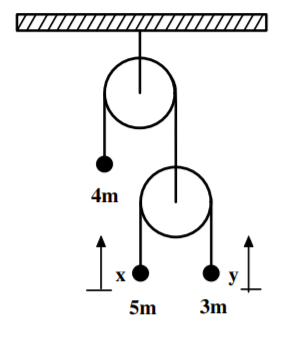
Consider the Atwoods machine shown. The masses are $4m$ , $5m$ , and $3m$ . Let $x$ and $y$ be the heights of the right two masses relative to their initial positions.
1. Solve this problem using the Euler-Lagrange equations b) Use Noether’s theorem to find the conserved momentum.
2. Use Noether’s theorem to find the conserved momentum.
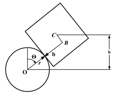
A cube of side
$2b$
and center of mass
$C$
, is placed on a fixed horizontal cylinder of radius
$r$
and center
$O$
as shown in the figure. Originally the cube is placed such that
$C$
is centered above
$O$
but it can roll from side to side without slipping. (a) Assuming that
$b<r$
use the Lagrangian approach to find the frequency for small oscillations about the top of the cylinder. For simplicity make the small angle approximation for
$L$
before using the Lagrange-Euler equations. (b) What will be the motion if
$b>r$
? Note that the moment of inertia of the cube about the center of mass is
$\frac{2}{3}mb^{2}$
.
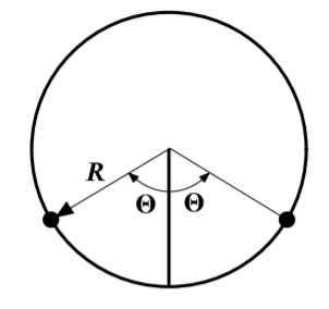
Two equal masses of mass
$m$
are glued to a massless hoop of radius
$R$
is free to rotate about its center in a vertical plane. The angle between the masses is
$2\theta$
, as shown. Find the frequency of oscillations.
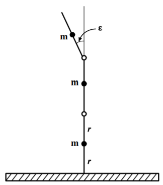
Three massless sticks each of length
$2r$
, and mass
$m$
with the center of mass at the center of each stick, are hinged at their ends as shown. The bottom end of the lower stick is hinged at the ground. They are held so that the lower two sticks are vertical, and the upper one is tilted at a small angle
$\varepsilon$
with respect to the vertical. They are then released. At the instant of release what are the three equations of motion derived from the Lagrangian derived assuming that
$\varepsilon$
is small
$?$
Use these to determine the initial angular accelerations of the three sticks.

7.S: Symmetries, Invariance and the Hamiltonian (Summary)¶

This chapter has explored the importance of symmetries and invariance in Lagrangian mechanics and has introduced the Hamiltonian. The following summarizes the important conclusions derived in this chapter.

Noether’s theorem:¶

Noether’s theorem explores the remarkable connection between symmetry, plus the invariance of a system under transformation, and related conservation laws which imply the existence of important physical principles, and constants of motion. Transformations where the equations of motion are invariant are called invariant transformations. Variables that are invariant to a transformation are called cyclic variables. It was shown that if the Lagrangian does not explicitly contain a particular coordinate of displacement, $q_{i}$ then the corresponding conjugate momentum, $\dot{p}_{i}$ is conserved. This is Noether’s theorem which states “ For each symmetry of the Lagrangian, there is a conserved quantity" . In particular it was shown that translational invariance in a given direction leads to the conservation of linear momentum in that direction, and rotational invariance about an axis leads to conservation of angular momentum about that axis. These are the first-order spatial and angular integrals of the equations of motion. Noether’s theorem also relates the properties of the Hamiltonian to time invariance of the Lagrangian, namely;

(1) $H$ is conserved if, and only if, the Lagrangian, and consequently the Hamiltonian, are not explicit functions of time.

(2) The Hamiltonian gives the total energy if the constraints and coordinate transformations are time independent and the potential energy is velocity independent. This is equivalent to stating that $H=E$ if the constraints, or generalized coordinates, for the system are time independent.

Noether’s theorem is of importance since it underlies the relation between symmetries, and invariance in all of physics; that is, its applicability extends beyond classical mechanics.

Generalized momentum:¶

The generalized momentum associated with the coordinate $q_{j}$ is defined to be

\frac{\partial L}{\partial \dot{q}_{j}}\equiv p_{j} \tag{7.3}

where $p_{j}$ is also called the conjugate momentum (orcanonical momentum) to $q_{j}$ where $q_{j},p_{j}$ are conjugate, or canonical, variables. Remember that the linear momentum $p_{j}$ is the first-order time integral given by equation $(3.4.1)$ . Note that if $q_{j}$ is not a spatial coordinate, then $p_{j}$ is not linear momentum, but is the conjugate momentum. For example, if $q_{j}$ is an angle, then $p_{j}$ will be angular momentum.

Kinetic energy in generalized coordinates:¶

It was shown that the kinetic energy can be expressed in terms of generalized coordinates by $$

\begin{align} T(\mathbf{q},\mathbf{ \dot{q}},t) &=&\sum_{\alpha }\sum_{i,j,k}\frac{1}{2}m_{\alpha }\frac{ \partial x_{\alpha ,i}}{\partial q_{j}}\frac{\partial x_{\alpha ,i}}{ \partial q_{k}}\dot{q}_{j}\dot{q}_{k}+\sum_{\alpha }\sum_{i,j}m_{\alpha } \frac{\partial x_{\alpha ,i}}{\partial q_{j}}\frac{\partial x_{\alpha ,i}}{ \partial t}\dot{q}_{j}+\sum_{\alpha }\sum_{i}\frac{1}{2}m_{\alpha }\left( \frac{\partial x_{\alpha ,i}}{\partial t}\right) ^{2} \tag{7.19} \\ &=&T_{2}(\mathbf{q},\mathbf{\dot{q}},t)+T_{1}(\mathbf{q},\mathbf{\dot{q}} ,t)+T_{0}(\mathbf{q},t)\end{align}

For scleronomic systems with a potential that is velocity independent, then the kinetic energy can be expressed as

T=T_{2}=\frac{1}{2}\sum_{l}\dot{q}_{l}p_{l}=\frac{1}{2}\mathbf{\dot{q}\cdot p } \tag{7.31}

Generalized energy¶

Jacobi’s Generalized Energy $h(\mathbf{q},\dot{q},t)$ was defined as

h(\mathbf{q},\mathbf{ \dot{q}},t)\equiv \sum_{j}\left( \dot{q}_{j}\frac{\partial L}{\partial \dot{q }_{j}}\right) -L(\mathbf{q},\mathbf{\dot{q}},t) \tag{7.36}

Hamiltonian function¶

The Hamiltonian $H\left( \mathbf{q,p,}t\right)$ was defined in terms of the generalized energy $h(\mathbf{q},\mathbf{\dot{q}},t)$ and by introducing the generalized momentum. That is

H\left( \mathbf{q,p,}t\right) \equiv h(\mathbf{q},\mathbf{\dot{q}} ,t)=\sum_{j}p_{j}\dot{q}_{j}-L(\mathbf{q},\mathbf{\dot{q}},t)=\mathbf{p\cdot \dot{q}-}L(\mathbf{q},\mathbf{\dot{q}},t) \tag{7.37}

Generalized energy theorem¶

The equations of motion lead to the generalized energy theorem which states that the time dependence of the Hamiltonian is related to the time dependence of the Lagrangian.

\frac{dH\left( \mathbf{q,p,}t\right) }{dt}=\sum_{j}\dot{q}_{j}\left[ Q_{j}^{EXC}+\sum_{k=1}^{m}\lambda _{k}\frac{\partial g_{k}}{\partial q_{j}}( \mathbf{q},t)\right] -\frac{\partial L(\mathbf{q},\mathbf{\dot{q}},t)}{ \partial t} \tag{7.38}

Note that if all the generalized non-potential forces are zero, then the bracket in Equation 7.38 is zero, and if the Lagrangian is not an explicit function of time, then the Hamiltonian is a constant of motion.

Generalized energy and total energy:¶

The generalized energy, and corresponding Hamiltonian, equal the total energy if:

The kinetic energy has a homogeneous quadratic dependence on the generalized velocities and the transformation to generalized coordinates is independent of time,** $\frac{\partial x_{\alpha ,i}}{\partial t}=0.$
The**potential energy is not velocity dependent,**thus the terms $\frac{\partial U}{\partial \dot{q}_{i}}=0.$

Chapter 8 will introduce Hamiltonian mechanics that is built on the Hamiltonian, and chapter 15 will explore applications of Hamiltonian mechanics.

Footnotes¶

Most textbooks call the function $h(\mathbf{q},\mathbf{\dot{q}},t)$ Jacobi’s energy integral. This book adopts the more descriptive name Generalized energy in analogy with use of generalized coordinates $\mathbf{q}$ and generalized momentum $\mathbf{p}$ .
↩