2. Review of Newtonian Mechanics

2.1: Introduction to Newtonian Mechanics¶

It is assumed that the reader has been introduced to Newtonian mechanics applied to one or two point objects. This chapter reviews Newtonian mechanics for motion of many-body systems as well as for macroscopic sized bodies. Newton’s Law of Gravitation also is reviewed. The purpose of this review is to ensure that the reader has a solid foundation of elementary Newtonian mechanics upon which to build the powerful analytic Lagrangian and Hamiltonian approaches to classical dynamics.

Newtonian mechanics is based on application of Newton’s Laws of motion which assume that the concepts of distance, time, and mass, are absolute, that is, motion is in an inertial frame. The Newtonian idea of the complete separation of space and time, and the concept of the absoluteness of time, are violated by the Theory of Relativity as discussed in chapter 17. However, for most practical applications, relativistic effects are negligible and Newtonian mechanics is an adequate description at low velocities. Therefore chapters $2-16$ will assume velocities for which Newton’s laws of motion are applicable.

2.2: Newton’s Laws of motion¶

Newton defined a vector quantity called linear momentum $\mathbf{p}$ which is the product of mass and velocity.

\tag{2.1} \mathbf{p} = m\dot{\mathbf{r}}

Since the mass $m$ is a scalar quantity, then the velocity vector $\dot{r}$ and the linear momentum vector $\mathbf{p}$ are colinear.

Newton’s laws, expressed in terms of linear momentum, are:

Law of inertia: A body remains at rest or in uniform motion unless acted upon by a force.
Equation of motion: A body acted upon by a force moves in such a manner that the time rate of change of momentum equals the force.
$\tag{2.2} \mathbf{F} = \frac{d\mathbf{p}}{dt}$
Action and reaction: If two bodies exert forces on each other these forces are equal in magnitude and opposite in direction.

Newton’s second law contains the essential physics relating the force $\mathbf{F}$ and the rate of change of linear momentum**** $\mathbf{p}$ .

Newton’s first law, the law of inertia, is a special case of Newton’s second law in that if

\tag{2.3} \mathbf{F}=\frac{d\mathbf{p}}{dt}=0

then $\mathbf{p}$ ****is a constant of motion.

Newton’s third law also can be interpreted as a statement of the conservation of momentum, that is, for a two particle system with no external forces acting,

\tag{2.4} \mathbf{F}_{12} = -\mathbf{F}_{21}

If the forces acting on two bodies are their mutual action and reaction, then Equation 2.4 simplifies to

\tag{2.5} \mathbf{F}_{12}=-\mathbf{F}_{21}= \frac{d\mathbf{p_1}}{dt}+ \frac{d\mathbf{p_2}}{dt} = \frac{d}{dt}(\mathbf{p_1+p_2}) = 0

This implies that the total linear momentum $\mathbf{P = p_1 + p_2}$ is a constant of motion. Combining Equations 2.1 and 2.2 leads to a second-order differential equation

\tag{2.6} \mathbf{F}=\frac{d\mathbf{p}}{dt}=m\frac{d^2\mathbf{r}}{dt^2}=m\mathbf{\ddot{r}}

Note that the force on a body $\mathbf{F}$ , and the resultant acceleration ${\bf a = \ddot{r}}$ are colinear. Appendix 19.3.2 gives explicit expressions for the acceleration ${\bf a}$ in cartesian and curvilinear coordinate systems. The definition of force depends on the definition of the mass $m$ . Newton’s laws of motion are obeyed to a high precision for velocities much less than the velocity of light. For example, recent experiments have shown they are obeyed with an error in the acceleration of $\Delta a \leq 5 \times 10^{-14}\mathit{m/s^2}$ .

2.3: Inertial Frames of reference¶

Aninertial frame of referenceis one in which Newton’s Laws of motion are valid. It is a non-accelerated frame of reference. An inertial frame must be homogeneous and isotropic. Physical experiments can be carried out in different inertial reference frames. The Galilean transformation provides a means of converting between two inertial frames of reference moving at a constant relative velocity. Consider two reference frames $O$ and $O'$ with $O'$ moving with constant relative velocity ${\bf V}$ at time $t$ . Figure 2.3.1 shows a Galilean transformation which can be expressed in vector form.

\begin{split} \mathbf{r'} & =\mathbf{r}-\mathbf{V}t \\ t' & = t \end{split}\tag{2.7}

Equation 2.7 gives the boost, assuming Newton’s hypothesis that the time is invariant to change of inertial frames of reference. Differentiation of this transformation gives

$$ \begin{split}

\mathbf{\dot{r}'} & =\mathbf{\dot{r}}-\mathbf{V}\

\mathbf{\ddot{r}'} & = \mathbf{\ddot{r}}

\end{split}\tag{2.8} \label{eq-2-8} $$

Note that the forces in the primed and unprimed inertial frames are related by

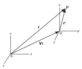
\tag{2.9} \mathbf{F}=\frac{d\mathbf{p}}{dt}=m\mathbf{\ddot{r}}=m\mathbf{\ddot{r}'}=\mathbf{F}'

Frame O' moving with a constant velocity V with respect to frame O at the time t. — Figure 2.3.1:Frame $O'$ moving with a constant velocity $V$ with respect to frame $O$ at the time $t$ .

Thus Newton’s Laws of motion are invariant under a Galilean transformation, that is, the inertial mass is unchanged under Galilean transformations. If Newton’s laws are valid in one inertial frame of reference, then they are valid in any frame of reference in uniform motion with respect to the first frame of reference. This invariance is called Galilean invariance. There are an infinite number of possible inertial frames all connected by Galilean transformations.

Galilean invariance violates Einstein’s Theory of Relativity. In order to satisfy Einstein’s postulate that the laws of physics are the same in all inertial frames, as well as satisfy Maxwell’s equations for electromagnetism, it is necessary to replace the Galilean transformation by the Lorentz transformation. As will be discussed in chapter 17, the Lorentz transformation leads to Lorentz contraction and time dilation both of which are related to the parameter $\gamma \equiv \frac{1}{\sqrt{1 - (\frac{v}{c})^2}}$ where c is the velocity of light in vacuum. Fortunately, most situations in life involve velocities where $v < < c$ ; for example, for a body moving at 25 000 mph (11 111 m/s) which is the escape velocity for a body at the surface of the earth, the $\gamma$ factor differs from unity by about $6.8 \times 10^{-10}$ which is negligible. Relativistic effects are significant only in nuclear and particle physics and some exotic conditions in astrophysics. Thus, for the purpose of classical mechanics usually it is reasonable to assume that the Galilean transformation is valid and is well obeyed under most practical conditions.

2.4: First-order Integrals in Newtonian mechanics¶

A fundamental goal of mechanics is to determine the equations of motion for an $n$ −body system, where the force ${\bf F}_i$ acts on the individual mass $m_i$ where $1 \leq i \leq n$ . Newton’s second-order equation of motion, equation $(2.2.6)$ must be solved to calculate the instantaneous spatial locations, velocities, and accelerations for each mass $m_i$ of an $n$ -body system. Both ${\bf F}_i$ and ${\bf \ddot{r}}_i$ are vectors each having three orthogonal components. The solution of equation $(2.2.6)$ involves integrating second-order equations of motion subject to a set of initial conditions. Although this task appears simple in principle, it can be exceedingly complicated for many-body systems. Fortunately, solution of the motion often can be simplified by exploiting three first-order integrals of Newton’s equations of motion, that relate directly to conservation of either the linear momentum, angular momentum, or energy of the system. In addition, for the special case of these three first-order integrals, the internal motion of any many-body system can be factored out by a simple transformations into the center of mass of the system. As a consequence, the following three first-order integrals are exploited extensively in classical mechanics.

Linear Momentum¶

Newton’s Laws can be written as the differential and integral forms of the first-order time integral which equals the change in linear momentum.

\tag{2.10} \mathbf{F}_i =\frac{d\mathbf{p}_i}{dt} \hspace{5cm} \int_1^2\mathbf{F}_idt = \int_1^2\frac{d\mathbf{p}_i}{dt}dt = ( \mathbf{p}_2 -\mathbf{p}_1)_i

This allows Newton’s law of motion to be expressed directly in terms of the linear momentum $\mathbf{p}_i = m_i\mathbf{\dot{r}}_i$ of each of the $1 < i < n$ bodies in the system. This first-order time integral features prominently in classical mechanics since it connects to the important concept of linear momentum ${\bf p}$ . This first-order time integral gives that the total linear momentum is a constant of motion when the sum of the external forces is zero.

Angular Momentum¶

The angular momentum ${\bf L}_i$ of a particle $i$ with linear momentum ${\bf p}_i$ with respect to an origin from which the position vector ${\bf r}_i$ is measured, is defined by

\tag{2.11} \mathbf{L}_i\equiv\mathbf{r}_i\times \mathbf{p}_i

The torque, or moment of the force $\mathbf{N}_i$ with respect to the same origin is defined to be

\tag{2.12} \mathbf{N}_i\equiv\mathbf{r}_i\times \mathbf{F}_i

where $\mathbf{r}_i$ is the position vector from the origin to the point where the force ${\bf F}_i$ is applied. Note that the torque ${\bf N}_i$ can be written as

\tag{2.13} \mathbf{N}_i\equiv\mathbf{r}_i\times\frac{d\mathbf{p}_i}{dt}

Consider the time differential of the angular momentum, $\frac{d\mathbf{L}_i}{dt}$

\tag{2.14} \frac{d\mathbf{L}_i}{dt}=\frac{d}{dt}( \mathbf{r}_i\times\mathbf{p}_i)=\frac{d\mathbf{r}_i}{dt}\times\mathbf{p}_i+\mathbf{r}_i\times\frac{d\mathbf{p}_i}{dt}

However,

\tag{2.15} \frac{d\mathbf{r}_i}{dt}\times\mathbf{p}_i=m\frac{d\mathbf{r}_i}{dt}\times\frac{d\mathbf{r}_i}{dt} = 0

Equations 2.13 − 2.15 can be used to write the first-order time integral for angular momentum in either differential or integral form as

$$ \tag{2.16} \label{eq-2-16}

\frac{d\mathbf{L}_i}{dt}=\mathbf{r}_i\times\frac{d\mathbf{p}_i}{dt}=\mathbf{N}_i \hspace{3cm} \int_1^2\mathbf{N}_idt = \int_1^2\frac{d\mathbf{L}_i}{dt}dt = ( \mathbf{L}_2 -\mathbf{L}_1)_i $$

Newton’s Law relates torque and angular momentum about the same axis. When the torque about any axis is zero then angular momentum about that axis is a constant of motion. If the total torque is zero then the total angular momentum, as well as the components about three orthogonal axes, all are constants.

Kinetic Energy¶

The third first-order integral, that can be used for solving the equations of motion, is the first-order spatial integral $\int_1^2\mathbf{F}_i \cdot d\mathbf{r}_i$ . Note that this spatial integral is a scalar in contrast to the first-order time integrals for linear and angular momenta which are vectors. The work done on a mass $m_i$ by a force $\mathbf{F}_i$ in transforming from condition 1 to 2 is defined to be

\tag{2.17} [W_{12} ] _i \equiv\int_1^2\mathbf{F}_i \cdot d\mathbf{r}_i

If ${\bf F}_i$ is the net resultant force acting on a particle $i$ then the integrand can be written as

\tag{2.18} F_i\cdot d\mathbf{r}_i = \frac{d\mathbf{p}_i}{dt}\cdot d\mathbf{r}_i = m_i\frac{d\mathbf{v}_i}{dt}\cdot\frac{d\mathbf{r}_i}{dt}dt=m_i\frac{d\mathbf{v}_i}{dt}\cdot\mathbf{v}_idt=\frac{m_i}{2}\frac{d}{dt}(\mathbf{v}_i\cdot\mathbf{v}_i ) dt = d\bigg(\frac{1}{2}m_iv_i^2\bigg) = d [ T ] _i

where the kinetic energy of a particle $i$ is defined as

\tag{2.19} [ T] _i \equiv \frac{1}{2}m_iv_i^2

Thus the work done on the particle $i$ , that is, $[W_{12}]_{i}$ equals the change in kinetic energy of the particle if there is no change in other contributions to the total energy such as potential energy, heat dissipation, etc. That is

\tag{2.20} [W_{12}]_{i}= \bigg[ \frac{1}{2}mv_2^2-\frac{1}{2}mv_1^2 \bigg]_i = [T_2 - T_1 ]_i

Thus the differential, and corresponding first integral, forms of the kinetic energy can be written as

$$ \tag{2.21} \label{eq-2-21}

\mathbf{F}_i = \frac{d\mathbf{T}_i}{dt} \hspace{5cm} \int_1^2\mathbf{F}_i \cdot d\mathbf{r}_i = ( \mathbf{T}_2 -\mathbf{T}_1)_i $$

If the work done on the particle is positive, then the final kinetic energy $T_2 > T_1$ Especially noteworthy is that the kinetic energy $[T]_i$ is a scalar quantity which makes it simple to use. This first-order spatial integral is the foundation of the analytic formulation of mechanics that underlies Lagrangian and Hamiltonian mechanics.

2.5: Conservation Laws in Classical Mechanics¶

Elucidating the dynamics in classical mechanics is greatly simplified when conservation laws are applicable. In nature, isolated many-body systems frequently conserve one or more of the first-order integrals for linear momentum, angular momentum, and mass/energy. Note that mass and energy are coupled in the Theory of Relativity, but for non-relativistic mechanics the conservation of mass and energy are decoupled. Other observables such as lepton and baryon numbers are conserved, but these conservation laws usually can be subsumed under conservation of mass for most problems in non-relativistic classical mechanics.

The power of conservation laws in calculating classical dynamics makes it useful to combine the conservation laws with the first integrals for linear momentum, angular momentum, and work-energy, when solving problems involving Newtonian mechanics. These three conservation laws will be derived assuming Newton’s laws of motion, however, these conservation laws are fundamental laws of nature that apply well beyond the domain of applicability of Newtonian mechanics.

2.6: Motion of finite-sized and many-body systems¶

Elementary presentations in classical mechanics discuss motion and forces involving single point particles. However, in real life, single bodies have a finite size introducing new degrees of freedom such as rotation and vibration, and frequently many finite-sized bodies are involved.

A finite-sized body can be thought of as a system of interacting particles such as the individual atoms of the body. The interactions between the parts of the body can be strong which leads to rigid body motion where the positions of the particles are held fixed with respect to each other, and the body can translate and rotate. When the interaction between the bodies is weaker, such as for a diatomic molecule, additional vibrational degrees of relative motion between the individual atoms are important. Newton’s third law of motion becomes especially important for such many-body systems.

2.7: Center of Mass of a Many-Body System¶

A finite sized body needs a reference point with respect to which the motion can be described. For example, there are 8 corners of a cube that could server as reference points, but the motion of each corner is complicated if the cube is both translating and rotating. The treatment of the behavior of finite-sized bodies, or many-body systems, is greatly simplified using the concept of center of mass. The center of mass is a particular fixed point in the body that has an especially valuable property; that is, the translational motion of a finite sized body can be treated like that of a point mass located at the center of mass. In addition the translational motion is separable from the rotational-vibrational motion of a many-body system when the motion is described with respect to the center of mass. Thus it is convenient at this juncture to introduce the concept of center of mass of a many-body system.

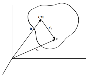
Figure 2.7.1:Position vector with respect to the center of mass.

For a many-body system, the position vector $\mathbf{r}_i$ , defined relative to the laboratory system, is related to the position vector $\mathbf{r}_i^\prime$ with respect to the center of mass, and the center-of-mass location $\mathbf{R}$ relative to the laboratory system. That is, as shown in Figure 2.7.1

\tag{2.22} \mathbf{r}_i = \mathbf{R} +\mathbf{r}^\prime_i

This vector relation defines the transformation between the laboratory and center of mass systems. For discrete and continuous systems respectively, the location of the center of mass is uniquely defined as being where

\tag{Center of mass definition}\sum^n_i m_i \mathbf{r}^\prime_i = \int \mathbf{r}^\prime \rho dV = 0

Define the total mass

\tag{Total mass}M=\sum_i^n m_i = \int_{body}\rho dV

The average location of the system corresponds to the location of the center of mass since $\frac{1}{M}\sum_im_i\mathbf{r}^\prime_i = 0$ that is

\tag{2.23} \frac{1}{M}\sum_im_i\mathbf{r}_i =\mathbf{R} + \frac{1}{M}\sum_im_i\mathbf{r}^\prime_i = \mathbf{R}

The vector $\mathbf{R}$ which describes the location of the center of mass, depends on the origin and coordinate system chosen. For a continuous mass distribution the location vector of the center of mass is given by

\tag{2.24} \mathbf{R}=\frac{1}{M}\sum_im_i\mathbf{r}_i=\frac{1}{M}\int\mathbf{r}\rho dV

The center of mass can be evaluated by calculating the individual components along three orthogonal axes.

The center-of-mass frame of referenceis defined as the frame for which the center of mass is stationary. This frame of reference is especially valuable for elucidating the underlying physics which involves only the relative motion of the many bodies. That is, the trivial translational motion of the center of mass frame, which has no influence on the relative motion of the bodies, is factored out and can be ignored. For example, a tennis ball $(0.06 \ kg )$ approaching the earth $( 6 \times 10^{24} \ kg )$ with velocity $v$ could be treated in three frames, (a) assume the earth is stationary, (b) assume the tennis ball is stationary, or (c) the center-of-mass frame. The latter frame ignores the center of mass motion which has no influence on the relative motion of the tennis ball and the earth. The center of linear momentum and center of mass coordinate frames are identical in Newtonian mechanics but not in relativistic mechanics as described in chapter 17.4.3.

2.8: Total Linear Momentum of a Many-body System¶

Center-of-mass decomposition¶

The total linear momentum $\mathbf{P}$ for a system of $n$ particles is given by

\tag{2.25} \mathbf{P}=\sum_i^n\mathbf{p}_i = \frac{d}{dt}\sum_i^nm_i\mathbf{r}_i

It is convenient to describe a many-body system by a position vector $\mathbf{r}^\prime_i$ with respect to the center of mass.

\tag{2.26} \mathbf{r}_i =\mathbf{R} + \mathbf{r}^\prime_i

That is,

\tag{2.27} \mathbf{P} = \sum_i^n\mathbf{p}_i = \frac{d}{dt}\sum_i^nm_i\mathbf{r}_i=\frac{d}{dt}M\mathbf{R}+ \frac{d}{dt}\sum_i^nm_i\mathbf{r}^\prime_i = \frac{d}{dt}M\mathbf{R}+0= M\mathbf{\dot R}

since $\sum_i^nm_i\mathbf{r}^\prime_i=0$ as given by th definition of the center of mass. That is,

\tag{2.28} \mathbf{P}=M\mathbf{\dot R}

Thus the total linear momentum for a system is the same as the momentum of a single particle of mass $M = \sum_i^n m_i$ located at the center of mass of the system.

Equations of motion¶

The force acting on particle $i$ in an $n$ -particle many-body system, can be separated into an external force $\mathbf{F}_i^{Ext}$ plus internal forces $\mathbf{f}_{ij}$ between the $n$ particles of the system

\tag{2.29} \mathbf{F}_i=\mathbf{F}_i^E + \sum_{\substack{j \\ i \neq j}}^n \mathbf{f}_{ij}

The origin of the external force is from outside of the system while the internal force is due to the mutual interaction between the $n$ particles in the system. Newton’s Law tells us that

\tag{2.30} \mathbf{\dot p}_i=\mathbf{F}_i = \mathbf{F}_i^E + \sum_{\substack{j \\ i \neq j}}^n \mathbf{f}_{ij}

Thus the rate of change of total momentum is

\tag{2.31} \mathbf{\dot{P}}=\sum_i^n\mathbf{\dot{p}}_i=\sum_i^n\mathbf{F}_i^E + \sum_i^n\sum_{\substack{j \\ i \neq j }}^n\mathbf{f}_{ij}

Note that since the indices are dummy then

\tag{2.32} \sum_i\sum_{\substack{j \\ i\neq j}}^n\mathbf{f}_{ij}=\sum_j\sum_{\substack{i \\ i \neq j}}^n\mathbf{f}_{ji}

Substituting Newton’s third law $\mathbf{f}_{ij} = -\mathbf{f}_{ji}$ into Equation 2.32 implies that

\tag{2.33} \sum_i\sum_{\substack{j \\ i \neq j }}^n\mathbf{f}_{ij}=\sum_{j}\sum_{\substack{i \\ i \neq j}}^n\mathbf{f}_{ji} = -\sum_i^n\sum_{\substack{j \\ i \neq j}}^n\mathbf{f}_{ij}=0

which is satisfied only for the case where the summations equal zero. That is, for every internal force, there is an equal and opposite reaction force that cancels that internal force.

Therefore the first-order integral for linear momentum can be written in differential and integral forms as

\tag{2.34} \mathbf{\dot{P}}=\sum_i^n\mathbf{F}_I^E \hspace{5cm}\int_1^2\sum_i^n\mathbf{F}_i^Edt = \mathbf{P}_2 - \mathbf{P}_1

The reaction of a body to an external force is equivalent to a single particle of mass M located at the center of mass assuming that the internal forces cancel due to Newton’s third law.

Note that the total linear momentum ${\bf P}$ is conserved if the net external force ${\bf F}^E$ is zero, that is

\tag{2.35} \mathbf{F}^E = \frac{d\mathbf{P}}{dt}= 0

Therefore the total linear momentum ${\bf P}$ of the center of mass is a constant. Moreover, if the component of the force along any direction ${\bf \hat{e}}$ is zero, that is,

\tag{2.36} \mathbf{F}^E\cdot {\bf \hat{e}} = \frac{d\mathbf{P}\cdot {\bf \hat{e}}}{dt}=0

then ${\bf P \cdot \hat{e}}$ is a constant. This fact is used frequently to solve problems involving motion in a constant force field. For example, in the earth’s gravitational field, the momentum of an object moving in vacuum in the vertical direction is time dependent because of the gravitational force, whereas the horizontal component of momentum is constant if no forces act in the horizontal direction.

Example 2.8.1: Exploding cannon shell

Consider a cannon shell of mass $M$ moves along a parabolic trajectory in the earths gravitational field. An internal explosion, generating an amount $E$ of mechanical energy, blows the shell into two parts. One part of mass $kM$ , where $k < 1$ , continues moving along the same trajectory with velocity $v^\prime$ while the other part is reduced to rest. Find the velocity of the mass $kM$ immediately after the explosion.

It is important to remember that the energy release $E$ is given in the center of mass. If the velocity of the shell immediately before the explosion is $v$ and $v^\prime$ is the velocity of the $kM$ part immediately after the explosion, then energy conservation gives that $\frac{1}{2}Mv^2 + E = \frac{1}{2}kMv^{\prime 2} T$ . The conservation of linear momentum gives $Mv = kMv^\prime$ . Eliminating $v$ from these equations gives

\nonumber v^\prime = \sqrt{\frac{2E}{ [ k (1-k) M ] }}

Figure 2.8.1:Exploding cannon shell

Example 2.8.2: Billiard-ball collisions

A billiard ball with mass $m$ and incident velocity $v$ collides with an identical stationary ball. Assume that the balls bounce off each other elastically in such a way that the incident ball is deflected at a scattering angle $\theta$ to the incident direction. Calculate the final velocities $v_f$ and $V_f$ of the two balls and the scattering angle $\phi$ of the target ball. The conservation of linear momentum in the incident direction $x$ , and the perpendicular direction give

mv = mv_f \cos \theta + mV_f \cos \phi \\ 0 = mv_f \sin \theta - mV_f \sin \phi \nonumber

Energy conservation gives.

\nonumber \frac{m}{2}v^2 = \frac{m}{2}v_f^2 + \frac{m}{2}V_f^2

Solving these three equations gives $\phi = 90^\circ - \theta$ , that is, the balls bounce off perpendicular to each other in the laboratory frame. The final velocities are

\nonumber v_f = v \cos \theta \\ V_f = v \sin \theta

2.9: Angular Momentum of a Many-Body System¶

Center-of-mass Decomposition¶

As was the case for linear momentum, for a many-body system it is possible to separate the angular momentum into two components. One component is the angular momentum about the center of mass and the other component is the angular motion of the center of mass about the origin of the coordinate system. This separation is done by describing the angular momentum of a many-body system using a position vector $\mathbf{r}_i^\prime$ with respect to the center of mass plus the vector location $\mathbf{R}$ of the center of mass.

\tag{2.37} \mathbf{r}_i = \mathbf{R} + \mathbf{r}_i^\prime

The total angular momentum

\mathbf{L} = \sum_{i}^n \mathbf{L}_i = \sum_{i}^n \mathbf{r}_i \times \mathbf{p}_i \\ = \sum_i^n ( \mathbf{R} + \mathbf{r}_i^\prime ) \times m_i ( \mathbf{\dot R} + \mathbf{\dot r}^\prime_i ) \\ = \sum_i^n m_i \big[\mathbf{r}_i^\prime \times \mathbf{\dot r}_i^\prime + \mathbf{r}_i^\prime \times \mathbf{\dot R} + \mathbf{R} \times \mathbf{\dot r}_i^\prime + \mathbf{R} \times \mathbf{\dot R} ]

Note that if the position vectors are with respect to the center of mass, then $\sum_i^n m_i \mathbf{r}_i^\prime = 0$ resulting in the middle two terms in the bracket being zero, that is;

\tag{2.39} \mathbf{L} = \sum_{i}^{n} \mathbf{r}^\prime_i \times \mathbf{p}^\prime_i + \mathbf{R} + \mathbf{P}

*The total angular momentum separates into two terms, the angular momentum about the center of mass, plus the angular momentum of the center of mass about the origin of the axis system.*This factoring of the angular momentum only applies for the center of mass. This is called Samuel König’s first theorem.

Equations of motion¶

The time derivative of the angular momentum

\tag{2.40} \mathbf{\dot L}_i = \frac{d}{dt}\mathbf{r}_i \times \mathbf{p}_i = \mathbf{\dot r}_i \times \mathbf{p}_i + \mathbf{r}_i \times \mathbf{\dot p}_i

\tag{2.41} \mathbf{\dot r}_i \times \mathbf{p}_i = m_i\mathbf{\dot r}_i\times \mathbf{\dot r}_i = 0

\tag{2.42} \mathbf{\dot L}_i = \mathbf{r}_i \times \mathbf{\dot p}_i = \mathbf{r}_i \times \mathbf{F}_i = \mathbf{N}_i

Consider that the resultant force acting on particle $i$ in this $n$ -particle system can be separated into an external force $\mathbf{F}_i^{Ext}$ plus internal forces between the $n$ particles of the system

\tag{2.43} \mathbf{F}_i = \mathbf{F}_i^E + \sum_{ \substack {j \\ i \neq j}}^{n} \mathbf{f} _{ij}

The origin of the external force is from outside of the system while the internal force is due to the interaction with the other $n -1$ particles in the system. Newton’s Law tells us that

\tag{2.44} \mathbf{\dot p}_i = \mathbf{F}_i = \mathbf{F}_i^E + \sum_{\substack {j \\ i \neq j}}^{n}\mathbf{f}_{ij}

The rate of change of total angular momentum is

\tag{2.45} \mathbf{\dot L} = \sum_i \mathbf{\dot L}_i = \sum_i \mathbf{r}_i \times \mathbf{\dot p}_i = \sum_i\mathbf{r}_i \times \mathbf{F}_i^E\ + \sum_i\sum_{\substack{j \\ i \neq j }}\mathbf{r}_i \times \mathbf{f}_{ij}

Since $\mathbf{f}_{ij} = -\mathbf{f}_{ji}$ the last expression can be written as

\tag{2.46} \sum_i \sum _{\substack{j \\ i \neq j}} \mathbf{r} _i \times \mathbf{f} _{ij} = \sum_i \sum _{\substack{j \\ i < j}} ( \mathbf{r}_i - \mathbf{r}_j ) \times \mathbf{f} _{ij}

Note that $( \mathbf{r}_i - \mathbf{r}_j )$ is the vector $\mathbf{r} _{ij}$ connecting $j$ to $i$ . For central forces the force vector $\mathbf{f}_{ij} = f_{ij} \widehat{\mathbf{r}_{ij}}$ thus

\tag{2.47} \sum_i\sum_{\substack{j \\ i < j}} ( \mathbf{r}_i - \mathbf{r}_j ) \times \mathbf{f}_{ij}= \sum_i\sum_{\substack{j \\ i < j }}\mathbf{r}_i \times \mathbf{f}_{ij } \hat{\mathbf{r}_{ij}}

That is, for central internal forces the total internal torque on a system of particles is zero, and the rate of change of total angular momentum for central internal forces becomes

\tag{2.48} \mathbf{\dot L} = \sum_i \mathbf{r}_i \times \mathbf{F}_i^E = \sum_i \mathbf{N}_i^E = \mathbf{N}^E

where $\mathbf{N}^E$ is the net external torque acting on the system. Equation 2.48 leads to the differential and integral forms of the first integral relating the total angular momentum to total external torque.

\tag{2.49} \mathbf{\dot L} = \mathbf{N}^E \hspace{5cm} \int_1^2 \mathbf{N}^E dt = \mathbf{L}_2 - \mathbf{L}_1

Angular momentum conservation occurs in many problems involving zero external torques $\mathbf{N}^E = 0$ plus two-body central forces $\mathbf{F} = f(r) \hat{\mathbf{r}}$ since the torque on the particle about the center of the force is zero

\tag{2.50} \mathbf{N}= \mathbf{r} \times \mathbf{F} = f(r) [ \mathbf{r} \times \mathbf{ \hat{r}} ] = 0

Examples are, the central gravitational force for stellar or planetary systems in astrophysics, and the central electrostatic force manifest for motion of electrons in the atom. In addition, the component of angular momentum about any axis $\mathbf{L} . \mathbf{\hat{e}}$ is conserved if the net external torque about that axis $\mathbf{N} . \mathbf{\hat{e}} = 0$ .

Example 2.9.1: Bolas thrown by gaucho

Consider the bolas thrown by a gaucho to catch cattle. This is a system with conserved linear and angular momentum about certain axes. When the bolas leaves the gaucho’s hand the center of mass has a linear velocity $\mathbf{V}$ and an angular momentum about the center of mass of $\mathbf{L}$ . If no external torques act, then the center of mass of the bolas will follow a typical ballistic trajectory in the earth’s gravitational field while the angular momentum vector $\mathbf{L}$ is conserved, that is, both in magnitude and direction. The tension in the ropes connecting the three balls does not impact the motion of the system as long as the ropes do not snap due to centrifugal forces.

Figure 2.9.1:Bolas thrown by a guacho.

Figure 2.9.2:A hunter using bolas while mounted on a horse. (Public Domain; Pearson Scott Foresman)

2.10: Work and Kinetic Energy for a Many-Body System¶

Center-of-mass kinetic energy¶

For a many-body system the position vector $\mathbf{r}^\prime_i$ with respect to the center of mass is given by.

\tag{2.51} \mathbf{r}_i = \mathbf{R} + \mathbf{r}^\prime_i

The location of the center of mass is uniquely defined as being at the location where $\int \rho \mathbf{r}^\prime_i dV = 0$ . The velocity of the $i^{th}$ particle can be expressed in terms of the velocity of the center of mass $\mathbf{\dot R}$ plus the velocity of the particle with respect to the center of mass $\mathbf{\dot r}^\prime_i$ . That is,

\tag{2.52} \mathbf{\dot{r}}_i = \mathbf{\dot{R}} + \mathbf{\dot{r}}^\prime_i

The total kinetic energy $T$ is

\tag{2.53} T = \sum_i^n \frac{1}{2}m_iv_i^2 = \sum_i^n\frac{1}{2}m_i\mathbf{\dot{r}}_i\cdot \mathbf{\dot{r}}_i = \sum_i^n\frac{1}{2}m_i\mathbf{\dot{r}}^\prime_i\cdot \mathbf{\dot{r}}^\prime_i + \bigg ( \frac{d}{dt} \sum_i m_I \mathbf{\dot{r}}^\prime_i \bigg ) \cdot \mathbf{\dot{R}} + \sum_i \frac{1}{2} m_i \mathbf{\dot{R}} \cdot \mathbf{\dot{R}}

For the special case of the center of mass, the middle term is zero since, by definition of the center of mass, $\sum_i m_i \mathbf{\dot{r}}^\prime_i$ .Therefore

\tag{2.54} T = \sum_i^n \frac{1}{2} m_i {v^\prime_i}^2 + \frac{1}{2}MV^2

Thus the total kinetic energy of the system is equal to the sum of the kinetic energy of a mass $M$ moving with the center of mass velocity plus the kinetic energy of motion of the individual particles relative to the center of mass. This is called Samuel König’s second theorem.

Note that for a fixed center-of-mass energy, the total kinetic energy $T$ has a minimum value of $\sum_i^n \frac{1}{2} m_i {v^\prime_i}^2$ when the velocity of the center of mass $V$ = 0. For a given internal excitation energy, the minimum energy required to accelerate colliding bodies occurs when the colliding bodies have identical, but opposite, linear momenta. That is, when the center-of-mass velocity $V$ = 0.

Conservative forces and Potential Energy¶

In general, the line integral of a force field $\mathbf{F}$ , that is, $\int_1^2 \mathbf{F} \cdot d\mathbf{r}$ is both path and time dependent. However, an important class of forces, called conservative forces, exist for which the following two facts are obeyed.

Time independence: The force depends only on the particle position $\mathbf{r}$ , that is, it does not depend on velocity or time.
**Path independence:**For any two points 1 and 2 , the work done by $\mathbf{F}$ is independent of the path taken between 1 and 2.

If forces are path independent, then it is possible to define a scalar field, called potential energy and denoted by $U( \mathbf{r} )$ that is only a function of position. The path independence can be expressed by noting that the integral around a closed loop is zero. That is

\tag{2.55} \oint \mathbf{F} \cdot d \mathbf{r} = 0

Applying Stokes theorem for a path-independent force leads to the alternate statement that the curl is zero.

See appendix $19.7.3C$ .

\tag{2.56} \nabla \times \mathbf{ F} = 0

Note that the vector product of two del operators $\nabla$ acting on a scalar field U equals

\tag{2.57} \nabla \times \nabla U = 0

Thus it is possible to express a path-independent force field as the gradient of a scalar field, $U$ , that is

\tag{2.58} \mathbf{F} = - \nabla U

Then the spatial integral

\tag{2.59} \int_1^2 \mathbf{F} \cdot d \mathbf{r} = - \int_1^2 ( \nabla U) \cdot d \mathbf{r} = U_1 - U_2

Thus for a path-independent force, the work done on the particle is given by the change in potential energy if there is no change in kinetic energy. For example, if an object is lifted against the gravitational field, then work is done on the particle and the final potential energy $U_2$ exceeds the initial potential energy, $U_1$ .

Total Mechanical Energy¶

Thetotal mechanical energy $E$ of a particle is defined as the sum of the kinetic and potential energies.

\tag{2.60} E = T + U

Note that the potential energy is defined only to within an additive constant since the force $\mathbf{F} = - \nabla U$ depends only on difference in potential energy. Similarly, the kinetic energy is not absolute since any inertial frame of reference can be used to describe the motion and the velocity of a particle depends on the relative velocities of inertial frames. Thus the total mechanical energy $E =T + U$ is not absolute.

If a single particle is subject to several path-independent forces, such as gravity, linear restoring forces, etc., then a potential energy $U_i$ can be ascribed to each of the $m$ forces where for each force $\mathbf{F}_i = - \nabla U_i$ . In contrast to the forces, which add vectorially, these scalar potential energies are additive, $U = \sum_i^m U_i$ . Thus the total mechanical energy for $m$ potential energies equals

\tag{2.61} E = T + U ( \mathbf{r} ) = T + \sum_i^m U_i ( \mathbf{r} )

The time derivative of the total mechanical energy $E =T + U$ equals

\tag{2.62} \frac{dE}{dt} = \frac{dT}{dt} + \frac{dU}{dt}

Equation (2.4.9) gave that $dT = \mathbf{F} \cdot d\mathbf{r}$ . Thus, the first term in Equation 2.62 equals

\tag{2.63} \frac{dT}{dt} = \mathbf{F} \cdot \frac{d\mathbf{r}}{dt}

The potential energy can be a function of both position and time. Thus the time difference in potential energy due to change in both time and position is given as

\tag{2.64} \frac{dU}{dt} = \sum_i \frac{\partial U}{\partial x_i} \frac{d x_i}{ dt} + \frac{\partial U}{\partial t} = ( \nabla U ) \cdot \frac{d \mathbf{r}}{dt} + \frac{\partial U}{\partial t}

The time derivative of the total mechanical energy is given using Equations 2.63 and 2.64 in Equation 2.62

\tag{2.65} \frac{dE}{dt} = \frac{dT}{dt} + \frac{dU}{dt} = \mathbf{F} \cdot \frac{d\mathbf{r}}{dt} + ( \nabla U ) \cdot \frac{d \mathbf{r}}{dt} + \frac{\partial U}{\partial t} = [\mathbf{F} + ( \nabla U ) ] \cdot \frac{d\mathbf{r}}{dt} + \frac{\partial U}{\partial t}

Note that if the field is path independent, that is $\nabla \times \mathbf{F} = 0$ then the force and potential are related by

\tag{2.66} \mathbf{F} = - \nabla U

Therefore, for path independent forces, the first term in the time derivative of the total energy in Equation 2.65 is zero. That is,

\tag{2.67} \frac{dE}{dt} = \frac{\partial U}{\partial t}

In addition, when the potential energy $U$ is not an explicit function of time, then $\frac{\partial U}{\partial t} = 0$ and thus the total energy is conserved. That is, for the combination of (a) path independence plus (b) time independence, then the total energy of a conservative field is conserved.

Note that there are cases where the concept of potential still is useful even when it is time dependent. That is, if path independence applies, i.e. $\mathbf{F} = - \nabla U$ at any instant. For example, a Coulomb field problem where charges are slowly changing due to leakage etc., or during a peripheral collision between two charged bodies such as nuclei.

Example 2.10.1: Central force

A particle of mass m moves along a trajectory given by $x =x_o \cos \omega_1 t \ and \ y_0 \sin \omega_2 t$ .

a) Find the x and y components of the force and determine the condition for which the force is a central force.

Differentiating with respect to time gives

\begin{align*} \dot{x} = - x_0 \omega_1 \sin ( \omega _1 t ) & & \ddot{x} = - x_0 \omega_1 ^2\cos ( \omega _1 t ) \\ \dot{y} = - y_0 \omega_1 \cos ( \omega _2 t ) & & \ddot{y} = - y_0 \omega_2 ^2\sin ( \omega _1 t ) \end{align*}

Newton’s second law gives

\nonumber \mathbf{F} = m ( \ddot{x} \hat{i} + \ddot{y} \hat{j} ) = - m \Big [ x_0 \omega_1 ^2 \cos ( \omega _1 t ) \hat{i} + y_0 \omega_2 ^2 \sin ( \omega _1 t ) \hat{j} \Big ] = - m \Big [ \omega_1 ^2 x \hat{i} + \omega_2 ^2 y \hat{j} \Big ]

Note that if $\omega_1 = \omega_2 = \omega$ then

\nonumber \mathbf{F} = -m \omega^2 [ x \hat{i} + y \hat{j} ] = - m\omega^2 \mathbf{r}

That is, it is a central force if $\omega_1 = \omega_2 = \omega$ .

b) Find the potential energy as a function of x and y.

Since

\nonumber \mathbf{F} = - \nabla U = - \bigg [ \frac{\partial U}{\partial x} \hat{i} + \frac{\partial U}{\partial y} \hat{j} \bigg ]

then

\nonumber U = \frac{1}{2} m ( \omega_1^2 x^2 + \omega _2 ^2 y^2 )

assuming that $U = 0$ at the origin.

c) Determine the kinetic energy of the particle and show that it is conserved.

The total energy

\nonumber E = T + U = \frac{1}{2} m ( \dot{x}^2 + \dot{y}_2 ) + \frac{1}{2} m ( \omega_1^2 x^2 + \omega_2^2 y^2 ) = \frac{1}{2} m (x_0^2 \omega_1 ^2 + y_0^2 \omega_2 ^2 )

since $\cos^2 \theta + \sin^2 \theta = 1$ . Thus the total energy $E$ is a constant and is conserved.

Total mechanical energy for conservative systems¶

Equation (2.4.11) showed that, using Newton’s second law, $\mathbf{F} = \frac{d\mathbf{p}}{dt}$ , the first-order spatial integral gives that the work done $W_{12}$ is related to the change in the kinetic energy. That is,

\tag{2.68} W_{12} \equiv \int_1^2 \mathbf{F} \cdot d \mathbf{r} = \frac{1}{2} m v_2^2 - \frac{1}{2}v_1^2 = T_2 - T_1

The work done $W_{12}$ also can be evaluated in terms of the known forces $\mathbf{F}_i$ in the spatial integral. Consider that the resultant force acting on particle $i$ in this $n$ -particle system can be separated into an external force $\mathbf{F}_i^{Ext}$ plus internal forces between the $n$ particles of the system

\tag{2.69} \mathbf{F}_i = \mathbf{F}_i^E + \sum_{\substack{j \\ i \neq j}}^n \mathbf{f}_{ij}

The origin of the external force is from outside of the system while the internal force is due to the interaction with the other $n − 1$ particles in the system. Newton’s Law tells us that

\tag{2.70} \mathbf{\dot{p}}_i = \mathbf{F}_i = \mathbf{F}_i^E + \sum_{\substack{j \\ i \neq j}}^n \mathbf{f}_{ij}

The work done on the system by a force moving from configuration $1 \rightarrow 2$ is given by

\tag{2.71} W_{1 \rightarrow 2} = \sum_i^n \int_1^2 \mathbf{F}_i^E \cdot d \mathbf{r}_i + \sum_i^n\sum_{\substack{ j \\ i \neq j}}^n \int_1^2 \mathbf{f}_{ij} \cdot d \mathbf{r}_i

Since $\mathbf{f}_{ij} = - \mathbf{f}_{ji}$ then

\tag{2.72} W_{1 \rightarrow 2} = \sum_i^n \int_1^2 \mathbf{F}_i^E \cdot d \mathbf{r}_i + \sum_i^n\sum_{\substack{ j \\ i < j}}^n \int_1^2 \mathbf{f}_{ij} \cdot ( d \mathbf{r}_i - d\mathbf{r}_j )

Where $d \mathbf{r}_i - d\mathbf{r}_j = d\mathbf{r}_{ij}$ is the vector from $j$ to $i$ .

Assume that both the external and internal forces are conservative, and thus can be derived from time independent potentials, that is

\tag{2.73} \mathbf{F}_i^E = - \nabla _i U_i^{Ext}

\tag{2.74} \mathbf{f}_{ij} = - \nabla_i U_{ij}^{Int}

Then

\begin{align} W_{1 \rightarrow 2} = - \sum_i^n \int_1^2 - \nabla _i U_i^{Ext} \cdot d \mathbf{r}_i + \sum_i^n\sum_{\substack{ j \\ i < j}}^n \int_1^2 - \nabla_i U_{ij}^{Int} \cdot d \mathbf{r}_i \nonumber\\ = \sum_i^n U_i^{Ext} (1) - \sum_i^n U_i ^{Ext} (2) + \sum_i^n U_i ^{Int} (1) - \sum_i^n U_i ^{Int} (2) \nonumber\\ = U^{Ext} (1) - U^{Ext} (2) + U^{Int} ( 1 ) - U^{Int} (2) \tag{2.75} \end{align}

Define the total external potential energy,

\tag{2.76} U^{Ext} = \sum_i^n U_i^{Ext}

and the total internal energy

\tag{2.77} U^{Int} = \sum_i^n U_i ^{Int}

Equating the two equivalent equations for $W_{1\rightarrow 2}$ , that is, Equations 2.68 and 2.75 gives that

\tag{2.78} W_{1\rightarrow 2} = T_2 - T_1 = U^{Ext} (1) - U^{Ext} (2) + U^{Int} ( 1 ) - U^{Int} ( 2 )

Regroup these terms in Equation 2.78 gives

\nonumber T_1 + U^{Ext} (1) + U^{Int}(1) = T_2 + U^{Ext} (2) + U^{Int} (2)

This shows that, for conservative forces, the total energy is conserved and is given by

\tag{2.79} E = T + U^{Ext} + U^{Int}

The three first-order integrals for linear momentum, angular momentum, and energy provide powerful approaches for solving the motion of Newtonian systems due to the applicability of conservation laws for the corresponding linear and angular momentum, plus energy conservation for conservative forces. In addition, the important concept of center-of-mass motion naturally separates out for these three first-order integrals. Although these conservation laws were derived assuming Newton’s Laws of motion, these conservation laws are more generally applicable, and these conservation laws surpass the range of validity of Newton’s Laws of motion. For example, in 1930 Pauli and Fermi postulated the existence of the neutrino in order to account for non-conservation of energy and momentum in $\beta$ -decay because they did not wish to relinquish the concepts of energy and momentum conservation. The neutrino was first detected in 1956 confirming the correctness of this hypothesis.

2.11: Virial Theorem¶

The virial theorem is an important theorem for a system of moving particles both in classical physics and quantum physics. The Virial Theorem is useful when considering a collection of many particles and has a special importance to central-force motion. For a general system of mass points with position vectors $\mathbf{r}_i$ and applied forces $\mathbf{F}_i$ , consider the scalar product $G$

\tag{2.80} G \equiv \sum_i \mathbf{p}_i \cdot \mathbf{r}_i

where $i$ sums over all particles. The time derivative of $G$ is

\tag{2.81} \frac{dG}{dt} = \sum_i \mathbf{p}_i \cdot \mathbf{ \dot{r}}_i + \sum_i \mathbf{\dot{p}}_i \cdot \mathbf{r}_i

However,

\tag{2.82} \sum_i \mathbf{p}_i \cdot \mathbf{ \dot{r}}_i = \sum_i m \mathbf{\dot{r}}_i \cdot \mathbf{ \dot{r}}_i = \sum_i mv^2 = 2T

Also, since $\mathbf{\dot{p}}_i = \mathbf{F}_i$

\tag{2.83} \sum_i \mathbf{\dot{p}}_i \cdot \mathbf{r}_i = \sum_i \mathbf{F}_i \cdot \mathbf{r}_i

Thus

\tag{2.84} \frac{dG}{dt} = 2T + \sum_i \mathbf{F}_i \cdot \mathbf{r}_i

The time average over a period $\tau$ is

\tag{2.85} \frac{1}{T} \int_0^\tau \frac{dG}{dt} dt = \frac{G ( \tau ) - G ( 0 ) }{ \tau } = \langle 2T \rangle + \Bigg \langle \sum_i \mathbf{F}_i \cdot \mathbf{r}_i \Bigg \rangle

where the $\langle \rangle$ brackets refer to the time average. Note that if the motion is periodic and the chosen time $\tau$ equals a multiple of the period, then $\frac{G ( \tau ) - G ( 0 ) }{ \tau } = 0$ . Even if the motion is not periodic, if the constraints and velocities of all the particles remain finite, then there is an upper bound to $G$ .This implies that choosing $\tau \rightarrow \infty$ means that $\frac{G ( \tau ) - G ( 0 ) }{ \tau } \rightarrow 0$ . In both cases the left-hand side of the equation tends to zero giving the virial theorem

\tag{2.86} \langle T \rangle = - \frac{1}{2} \Bigg \langle \sum_i \mathbf{F}_i \cdot \mathbf{r}_i \Bigg \rangle

The right-hand side of this equation is called the virial of the system. For a single particle subject to a conservative central force $\mathbf{F} = - \nabla U$ the Virial theorem equals

\tag{2.87} \langle T \rangle = \frac{1}{2} \langle \nabla U \cdot \mathbf{r} \rangle = \frac{1}{2} \bigg \langle r \frac{\partial U}{\partial r} \bigg \rangle

If the potential is of the form $U = kr^{n+1}$ that is, $F = -k(n+1)r^{n}$ , then $r\frac{\partial U}{\partial r} = (n+1) U$ . Thus for a single particle in a central potential $U = kr^{n+1}$ the Virial theorem reduces to

\tag{2.88} \langle T \rangle = \frac{n+1}{2} \langle U \rangle

The following two special cases are of considerable importance in physics.

**Hooke’s Law:**Note that for a linear restoring force $n = 1$ then

\nonumber \tag{n=1} \langle T \rangle = + \langle U \rangle

You may be familiar with this fact for simple harmonic motion where the average kinetic and potential energies are the same and both equal half of the total energy.

Inverse-square law: The other interesting case is for the inverse square law $n = −2$ where

\nonumber \tag{n = -2} \langle T \rangle = - \frac{1}{2} \langle U \rangle

The Virial theorem is useful for solving problems in that knowing the exponent $n$ of the field makes it possible to write down directly the average total energy in the field. For example, for

\begin{align} \langle E \rangle &= \langle T \rangle + \langle U \rangle \\[4pt] &= -\frac{1}{2} \langle U \rangle + \langle U \rangle = \frac{1}{2} \langle U \rangle \tag{2.89} \end{align}

This occurs for the Bohr model of the hydrogen atom where the kinetic energy of the bound electron is half of the potential energy. The same result occurs for planetary motion in the solar system.

Example 2.11.1: The ideal gas law

The Virial theorem deals with average properties and has applications to statistical mechanics. Consider an ideal gas. According to the equipartition theorem the average kinetic energy per atom in an ideal gas is $\frac{3}{2} k T$ where $T$ is the absolute temperature and $k$ is the Boltzmann constant. Thus the average total kinetic energy for $N$ atoms is $\langle KE \rangle = \frac{3}{2}NkT$ . The right-hand side of the Virial theorem contains the force $\mathbf{F}_i$ . For an ideal gas it is assumed that there are no interaction forces between atoms, that is the only force is the force of constraint of the walls of the pressure vessel. The pressure $P$ is force per unit area and thus the instantaneous force on an area of wall $dA$ is $d\mathbf{F}_i = - \mathbf{\hat{n}}PdA$ where $\hat{n}$ designates the unit vector normal to the surface. Thus the right-hand side of the Virial theorem is

\nonumber -\frac{1}{2} \Bigg \langle \sum_i \mathbf{F}_i \cdot \mathbf{r}_i \Bigg \rangle = \frac{P}{2} \int \mathbf{\hat{n}} \cdot \mathbf{r}_i dA

Use of the divergence theorem thus gives that $\int \mathbf{\hat{n}} \cdot \mathbf{r}_i dA = \int \nabla \cdot \mathbf{r} dV = 3 \int dV =3V$ . Thus the Virial theorem leads to the ideal gas law, that is

\nonumber NkT = PV

Example 2.11.2: The mass of galaxies

The Virial theorem can be used to make a crude estimate of the mass of a cluster of galaxies. Assuming a spherically-symmetric cluster of $N$ galaxies, each of mass $m$ then the total mass of the cluster is $M = Nm$ . A crude estimate of the cluster potential energy is

\nonumber \tag{$\alpha$} \langle U \rangle \approx \frac{GM^2}{R}

where $R$ is the radius of a cluster. The average kinetic energy per galaxy is $\frac{1}{2} m \langle v \rangle ^2$ where $\langle v \rangle ^2$ is the average square of the galaxy velocities with respect to the center of mass of the cluster. Thus the total kinetic energy of the cluster is

\nonumber \tag{$\beta$} \langle KE \rangle \approx \frac{N m \langle v \rangle ^2 }{2} = \frac{M \langle v \rangle ^2 }{2}

The Virial theorem tells us that a central force having a radial dependence of the form $F \propto r^n$ gives $\langle KE \rangle = \frac{n+1}{2} \langle U \rangle$ . For the inverse-square gravitational force then

\nonumber \tag{$\gamma$} \langle KE \rangle = - \frac{1}{2} \langle U \rangle.

Thus equations $\alpha, \ \beta$ , and $\gamma$ give an estimate of the total mass of the cluster to be

\nonumber M \approx \frac{R \langle v \rangle ^2}{G}

This estimate is larger than the value estimated from the luminosity of the cluster implying a large amount of “dark matter” must exist in galaxies which remains an open question in physics.

2.12: Applications of Newton’s Equations of Motion¶

Newton’s equation of motion can be written in the form

\tag{2.90} \mathbf{F} = \frac{d\mathbf{p}}{dt} = m\frac{d\mathbf{v}}{dt} = m\frac{d^2\mathbf{r}}{dt^2}

A description of the motion of a particle requires a solution of this second-order differential equation of motion. This equation of motion may be integrated to find $\mathbf{r}(t)$ and $\mathbf{v}(t)$ if the initial conditions and the force field $\mathbf{F}(t)$ are known. Solution of the equation of motion can be complicated for many practical examples, but there are various approaches to simplify the solution. It is of value to learn efficient approaches to solving problems.

The following sequence is recommended

Make a vector diagram of the problem indicating forces, velocities, etc.
Write down the known quantities.
Before trying to solve the equation of motion directly, look to see if a basic conservation law applies. That is, check if any of the three first-order integrals, can be used to simplify the solution. The use of conservation of energy or conservation of momentum can greatly simplify solving problems.

The following examples show the solution of typical types of problem encountered using Newtonian mechanics

Constant Force Problems¶

Problems having a constant force imply constant acceleration. The classic example is a block sliding on an inclined plane, where the block of mass $m$ is acted upon by both gravity and friction. The net force $\mathbf{F}$ is given by the vector sum of the gravitational force $\mathbf{F}_g$ , normal force $\mathbf{N}$ and frictional force $\mathbf{f}_f$

\tag{2.91} \mathbf{F} = \mathbf{F}_g + \mathbf{N + f}_f = m\mathbf{a}

Taking components perpendicular to the inclined plane in the $y$ direction

\tag{2.92} -F_g \cos \theta + N = 0

That is, since $F_g = mg$

\tag{2.93} N = mg \cos \theta

Similarly, taking components along the inclined plane in the $x$ direction

\tag{2.94} F_g \sin \theta - f_f = m \frac{d^2 x}{dt^2}

Using the concept of coefficient of friction $\mu$

\tag{2.95} f_f = \mu N

Thus the equation of motion can be written as

\tag{2.96} mg( \sin \theta - \mu \cos \theta ) = m \frac{d^2 x}{dt^2}

The block accelerates if $\sin \theta > \mu \cos \theta$ , that is, $\tan \theta > \mu$ . The acceleration is constant if $\mu$ and $\theta$ are constant, that is

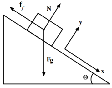
\tag{2.97} \frac{d^2x}{dt^2} = g ( \sin \theta - \mu \cos \theta )

Figure 2.12.1:Block on an inclined plane

Remember that if the block is stationary, the friction coefficient balances such that $( \sin \theta - \mu \cos \theta ) = 0$ that is, $\tan \theta = \mu$ . However, there is a maximum static friction coefficient $\mu _S$ beyond which the block starts sliding. The kinetic coefficient of friction $\mu_K$ is applicable for sliding friction and usually $\mu_K < \mu_S$

Another example of constant force and acceleration is motion of objects free falling in a uniform gravitational field when air drag is neglected. Then one obtains the simple relations such $v = u + at$ , etc.

Linear Restoring Force¶

An important class of problems involve a linear restoring force, that is, they obey Hooke’s law. The equation of motion for this case is

\tag{2.98} F ( x ) = -kx = m \ddot{x}

It is usual to define

\tag{2.99} \omega_0 ^2 \equiv \frac{k}{m}

Then the equation of motion then can be written as

\tag{2.100} \ddot{x} + \omega_0^2 x = 0

which is the equation of the harmonic oscillator. Examples are small oscillations of a mass on a spring, vibrations of a stretched piano string, etc.

The solution of this second order equation is

\tag{2.101} x(t) = A \sin ( \omega _0 t - \delta )

This is the well known sinusoidal behavior of the displacement for the simple harmonic oscillator. The angular frequency $\omega_0$

\tag{2.102} \omega_0 = \sqrt{\frac{k}{m}}

Note that for this linear system with no dissipative forces, the total energy is a constant of motion as discussed previously. That is, it is a conservative system with a total energy $E$ given by

\tag{2.103} \frac{1}{2} m \dot{x} ^2 + \frac{1}{2} kx ^2 = E

The first term is the kinetic energy and the second term is the potential energy. The Virial theorem gives that for the linear restoring force the average kinetic energy equals the average potential energy.

Position-dependent conservative forces¶

The linear restoring force is an example of a conservative field. The total energy $E$ is conserved, and if the field is time independent, then the conservative forces are a function only of position. The easiest way to solve such problems is to use the concept of potential energy $U$ illustrated in Figure 2.12.2.

\tag{2.104} U_2 - U_1 = - \int_1^2 \mathbf{F} \cdot d \mathbf{x}

Consider a conservative force in one dimension. Since it was shown that the total energy $E = T + U$ is conserved for a conservative field, then

\tag{2.105} E = T + U = \frac{1}{2} mv^2 + U (x)

Therefore:

\tag{2.106} v = \frac{dx}{dt} = \pm \sqrt{\frac{2}{m} [ E - U (x) ] }

Integration of this gives

\tag{2.107} t - t_0 = \int_{x_0}^x \frac{\pm dx}{\sqrt{\frac{2}{m} [ E - U (x) ]}}

where $x = x_0$ when $t = t_0$ Knowing $U(x)$ it is possible to solve this equation as a function of time.

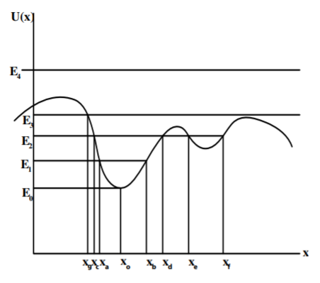
One-dimensional potential U(x). — Figure 2.12.2:One-dimensional potential $U(x)$ .

It is possible to understand the general features of the solution just from inspection of the function $U(x)$ . For example, as shown in Figure 2.12.2 the motion for energy $E_1$ is periodic between the turning points $x_a$ and $x_b$ . Since the potential energy curve is approximately parabolic between these limits the motion will exhibit simple harmonic motion. For $E_0$ the turning point coalesce to $x_0$ that is there is no motion. For total energy $E_2$ the motion is periodic in two independent regimes, $x_c \leq x \leq x_d$ and $x_e \leq x \leq x_f$ . Classically the particle cannot jump from one pocket to the other. The motion for the particle with total energy $E_3$ is that it moves freely from infinity, stops and rebounds at $x = x_g$ and then returns to infinity. That is the particle bounces off the potential at $x_g$ . For energy $E _4$ the particle moves freely and is unbounded. For all these cases, the actual velocity is given by the above relation for $v (x)$ . Thus the kinetic energy is largest where the potential is deepest. An example would be motion of a roller coaster car.

Position-dependent forces are encountered extensively in classical mechanics. Examples are the many manifestations of motion in gravitational fields, such as interplanetary probes, a roller coaster, and automobile suspension systems. The linear restoring force is an especially simple example of a position-dependent force while the most frequently encountered conservative potentials are in electrostatics and gravitation for which the potentials are;

\nonumber \tag{Electrostatic Potential energy} U(r) = \frac{1}{4 \pi \epsilon _0} \frac{q_1 q_2}{r_{12}^2}

\nonumber \tag{Gravitational Potential energy} U(r) = -G \frac{m_1 m_2}{r_{12}^2}

Knowing $U (r)$ it is possible to solve the equation of motion as a function of time.

Example 2.12.1: Diatomic molecule

An example of a conservative field is a vibrating diatomic molecule which has a potential energy dependence with separation distance $x$ that is described approximately by the Morse function

\nonumber U(x) = U_0 \Big [ 1 - e^{ - \frac{ ( x - x_0 )}{ \delta }} \Big ] ^2 - U_0

where $U_0, x_0 \ and \ \delta$ are parameters chosen to best describe the particular pair of atoms. The restoring force is given by

\nonumber F(x) = - \frac{dU(x)}{dx} = 2 \frac{U_0}{ \delta } \Big [ 1 - e^{- \frac{ ( x - x_0 )}{ \delta }} \Big ] \Big [ e^{- \frac{ ( x - x_0 )}{ \delta }} \Big ]

This has a minimum value of $U (x_0) = U_0$ at $x = x_0$ .

$Potential energy function U(x)/U_0 versus x/\delta for the diatomic molecule.$

Figure 2.12.3:Potential energy function $U(x)/U_0$ versus $x/\delta$ for the diatomic molecule.

Note that for small amplitude oscillations, where

\nonumber ( x - x_0 ) < < \delta

the exponential term in the potential function can be expanded to give

\nonumber U(x) \approx U_0 \Bigg [ 1 - (1 - -\frac{ (x - x_0 )}{ \delta}) \Bigg ] ^2 - U_0 \approx \frac{U_0}{\delta ^2} ( x - x_0 ) ^2 - U_0

This gives a restoring force

\nonumber F(x) = - \frac{dU(x)}{dx} = - 2 \frac{U_0}{ \delta} ( x - x_0 )

That is, for small amplitudes the restoring force is linear.

Constrained Motion¶

A frequently encountered problem with position dependent forces is when the motion is constrained to follow a certain trajectory. Forces of constraint must exist to constrain the motion to a specific trajectory. Examples are, the roller coaster, a rolling ball on an undulating surface, or a downhill skier, where the motion is constrained to follow the surface or track contours. The potential energy can be evaluated at all positions along the constrained trajectory for conservative forces such as gravity. However, the additional forces of constraint that must exist to constrain the motion, can be complicated and depend on the motion. For example, the roller coaster must always balance the gravitational and centripetal forces. Fortunately forces of constraint $\mathbf{F}_C$ often are normal to the direction of motion and thus do not contribute to the total mechanical energy since then the work done $\mathbf{F} _C \cdot d \mathbf{l}$ is zero. Magnetic forces $\mathbf{F} =q\mathbf{v} \times \mathbf{B}$ exhibit this feature of having the force normal to the motion.

Solution of constrained problems is greatly simplified if the other forces are conservative and the forces of constraint are normal to the motion, since then energy conservation can be used.

Example 2.12.2: Roller coaster

Consider motion of a roller coaster shown in the adjacent figure.

Figure 2.12.4:Roller coaster (CCO Public Domain)

This system is conservative if the friction and air drag are neglected and then the forces of constraint are normal to the direction of motion. The kinetic energy at any position is just given by energy conservation and the fact that

\nonumber E = T + U

where $U$ depends on the height of the track at any the given location. The kinetic energy is greatest when the potential energy is lowest. The forces of constraint can be deduced if the velocity of motion on the track is known. Assuming that the motion is confined to a vertical plane, then one has a centripetal force of constraint $\frac{mv^2}{ \rho }$ normal to the track inwards towards the center of the radius of curvature $\rho$ , plus the gravitation force downwards of $mg$ .

The constraint force is $\frac{mv^2_T}{ \rho } - mg$ upwards at the top of the loop, while it is $\frac{mv^2_B}{ \rho } + mg$ downwards at the bottom of the loop. To ensure that the car and occupants do not leave the required trajectory, the force upwards at the top of the loop has to be positive, that is, $v^2_T \geq \rho g$ . The velocity at the bottom of the loop is given by $\frac{1}{2} m v^2_B = \frac{1}{2}mv_T^2 + 2mg \rho$ assuming that the track has a constant radius of curvature $\rho$ . That is; at a minimum $v^2 _B = \rho g + 4 \rho g = 5 \rho g$ Therefore the occupants now will feel an acceleration downwards of at least $\frac{v^2_B}{\rho} + g = 6g$ at the bottom of the loop. The first roller coaster was built with such a constant radius of curvature but an acceleration of $6g$ was too much for the average passenger. Therefore roller coasters are designed such that the radius of curvature is much larger at the bottom of the loop, as illustrated, in order to maintain sufficiently low $g$ loads and also ensure that the required constraint forces exist.

Note that the minimum velocity at the top of the loop, $v_T$ , implies that if the cart starts from rest it must start at a height $h \geqslant \frac{\rho}{2}$ above the top of the loop if friction is negligible. Note that the solution for the rolling ball on such a roller coaster differs from that for a sliding object since one must include the rotational energy of the ball as well as the linear velocity.

Looping the loop in a glider involves the same physics making it necessary to vary the elevator control to vary the radius of curvature throughout the loop to minimize the maximum $g$ load.

Velocity Dependent Forces¶

Velocity dependent forces are encountered frequently in practical problems. For example, motion of an object in a fluid, such as air, where viscous forces retard the motion. In general the retarding force has a complicated dependence on velocity. The drag force usually is expressed in terms of a drag coefficient $c_D$ ,

\tag{2.108} \mathbf{F}_D(v) = -\frac{1}{2} c_D \rho A v^2 \mathbf{\hat{v}}

where $c_D$ is a dimensionless drag coefficient, $\rho$ is the density of air, $A$ is the cross sectional area perpendicular to the direction of motion, and $v$ is the velocity. Modern automobiles have drag coefficients as low as 0.3. As described in chapter 16, the drag coefficient $c_D$ depends on the Reynold’s number which relates the inertial to viscous drag forces. Small sized objects at low velocity, such as light raindrops, have low Reynold’s numbers for which $c_D$ is roughly proportional to $v^{-1}$ leading to a linear dependence of the drag force on velocity, i.e. $F_D (v) \propto v$ . Larger objects moving at higher velocities, such as a car or sky-diver, have higher Reynold’s numbers for which $c_D$ is roughly independent of velocity leading to a drag force $F_D (v) \propto v^2$ . This drag force always points in the opposite direction to the unit velocity vector. Approximately for air

\tag{2.109} \mathbf{F}_D(v) = -(c_1v + c_2 v^2 ) \hat{v}

where for spherical objects of diameter $D, c_1 \approx 1.55 \times 10^{-4} D$ and $c_2 \approx 0.22D^2$ and in MKS units. Fortunately, the equation of motion usually can be integrated when the retarding force has a simple power law dependence. As an example, consider free fall in the Earth’s gravitational field.

Example 2.12.3: Vertical fall in the earth’s gravitational field.

Linear regime $c_1 > > c_2 v$

For small objects at low-velocity, i.e. low Reynold’s number, the drag has approximately a linear dependence on velocity. The equation of motion is

\nonumber -mg -c_1 v =m \frac{dv}{dt}

Separate the variables and integrate

\nonumber t = \int_{v_0}^v \frac{m dv}{-mg - c_1 v } = -\frac{m}{c_1} \ln \bigg ( \frac{mg + c_1 v}{mg + c_1v_0} \bigg )

That is

\nonumber v = -\frac{mg}{c_1} + \bigg ( \frac{mg}{c_1} + v_0 \bigg ) e^{-\frac{c_1}{m} t}

Note that for $t \gg \frac{m}{c_1}$ the velocity approaches a terminal velocity of $v_\infty = -\frac{mg}{c_1}$ . The characteristic time constant is $\tau = \frac{m}{c_1} = \frac{v_\infty}{g}$ . Note that if $v_0 = 0$ , then

\nonumber v = v_\infty \Big ( 1 - e^{-\frac{t}{\tau}} \Big )

For the case of small raindrops with $D = 0.5 mm$ then $v_\infty = 8 \ m/s \ (18 \ mph)$ and time constant $\tau = 0.8 s$ . Note that in the absence of air drag, these rain drops falling from 2000 m would attain a velocity of over 400 mph. It is fortunate that the drag reduces the speed of rain drops to non-damaging values. Note that the above relation would predict high velocities for hail. Fortunately, the drag increases quadratically at the higher velocities attained by large rain drops or hail, and this limits the terminal velocity to moderate values. As known in the mid-west, these velocities still are sufficient to do considerable crop damage.

Quadratic regime $\hspace{4 cm} c_2v > > c_1$

For larger objects at higher velocities, i.e. high Reynold’s number, the drag depends on the square of the velocity making it necessary to differentiate between objects rising and falling. The equation of motion is

\nonumber -mg \pm c_2v^2 = m\frac{dv}{dt}

where the positive sign is for falling objects and negative sign for rising objects. Integrating the equation of motion for falling gives

\nonumber t = \int_{v_0}^v \frac{mdv}{-mg + c_2v^2} = \tau \bigg ( \tanh^{-1} \frac{v_0}{v_\infty} - \tanh^{-1} \frac{v}{v_\infty} \bigg )

where $\tau = \sqrt{\frac{m}{c_2g}}$ and $v_\infty = \sqrt{\frac{mg}{c_2}}$ That is, $\tau = \frac{v_\infty}{g}$ For the case of a falling object with $v_0 = 0$ solving for velocity gives

v = v_\infty \tanh \frac{t}{ \tau} \nonumber

As an example, a 0.6 kg basket ball with $D$ = 0.25 m will have $v_\infty = 20 m/s$ ( 43 mph) and $\tau = 2.1 \ s$ .

Consider President George H.W. Bush skydiving. Assume his mass is 70 kg and assume an equivalent spherical shape of the former President to have a diameter of $D = 1 \ m$ This gives that $v_\infty = 56 \ m/s$ ( 120 mph) and $\tau = 5.6 \ s$ . When Bush senior opens his 8 m diameter parachute his terminal velocity is estimated to decrease to 7m/s ( 15 mph) which is close to the value for a typical ( 8m) diameter emergency parachute which has a measured terminal velocity of 11 mph in spite of air leakage through the central vent needed to provide stability.

Example 2.12.4: Projectile motion in air

Consider a projectile initially at $x = y = 0$ , at $t = 0$ , that is fired at an initial velocity v $v_0$ at an angle $\theta$ to the horizontal. In order to understand the general features of the solution, assume that the drag is proportional to velocity. This is incorrect for typical projectile velocities, but simplifies the mathematics. The equations of motion can be expressed as

\nonumber m \ddot{x} = - km \ddot{x}

\nonumber m \ddot{y} = - km \dot{y} - mg

where k is the coefficient for air drag. Take the initial conditions at $t = 0$ to be $x = y = 0$ , $\dot{x} = v_o \cos \theta, \dot{y} = v_o \sin \theta$ .

Solving in the $x$ coordinate,

\nonumber \frac{ d\mathbf{x} }{dt} = -k \dot{x}

Therefore

\nonumber \dot{x} = v_o \cos \theta e ^{-kt}

That is, the velocity decays to zero with a time constant $\tau = \frac{1}{k}$

Integration of the velocity equation gives

\nonumber x = \frac{v_o}{k} ( 1 - e ^{-kt} )

Note that this implies that the body approaches a value of $x =\frac{v_o}{k}$ as $t \rightarrow \infty$

The trajectory of an object is distorted from the parabolic shape, that occurs for $k = 0$ , due to the rapid drop in range as the drag coefficient increases. For realistic cases it is necessary to use a computer to solve this numerically.

Systems with Variable Mass¶

Classic examples of systems with variable mass are the rocket, nuclear fission and other modes of nuclear decay.

Consider the problem of rocket motion in a gravitational field. When there is a vertical gravitational external field the vertical momentum is not conserved due to both gravity and the ejection of rocket propellant. In a time $dt$ the rocket ejects propellant $dm_p$ with exhaust velocity relative to the rocket of $u$ . Thus the momentum imparted to this propellant is

\tag{2.110} dp_p = -udm_p

Therefore the rocket is given an equal and opposite increase in momentum

\tag{2.111} dp_R = +udm_p

In the time interval $dt$ the net change in the linear momentum of the rocket plus fuel system is given by

\tag{2.112} dp = (m - dm_p ) ( v + dv) + dm_p (v - u ) - mv = mdv - udm_p

The rate of change of the linear momentum thus equals

\nonumber F_{ex} = \frac{dp}{dt} = m\frac{dv}{dt} - u \frac{dm_p}{dt}

Consider the problem for the special case of vertical ascent of the rocket against the external gravitational force $F_{ex} = -mg$ . Then

\tag{2.113} -mg + u\frac{dm_p}{dt} = m\frac{dv}{dt}

This can be rewritten as

\tag{2.114} -mg + u\dot{m}_p = m\dot{v}

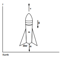
Figure 2.12.5:Vertical motion of a rocket in a gravitational field

The second term comes from the variable mass. But the loss of mass of the rocket equals the mass of the ejected propellant. Assuming a constant fuel burn $\dot{m}_p = \alpha$ then

\tag{2.115} \dot{m} = -\dot{m}_p = -\alpha

where $\alpha > 0$ Then the equation becomes

\tag{2.116} dv = \big ( -g + \frac{ \alpha}{m} u \big ) dt

Since

\tag{2.117} \frac{dm}{dt} = -\alpha

then

\tag{2.118} - \frac{dm}{\alpha} = dt

Inserting this in the above equation gives

\tag{2.119} dv = \big ( \frac{g}{\alpha} - \frac{u}{m} \big ) dm

Integration gives

\tag{2.120} v = - \frac{g}{\alpha} ( m_0 - m ) + u \ln \big ( \frac{m_0}{m} \big )

But the change in mass is given by

\tag{2.121} \int_{m_0}^m dm = - \alpha \int_0^t dt

That is

\tag{2.122} m_0 - m = \alpha t

Thus

\tag{2.123} v = -gt + u \ln \big ( \frac{m_0}{m} \big )

Note that once the propellant is exhausted the rocket will continue to fly upwards as it decelerates in the gravitational field. You can easily calculate the maximum height. Note that this formula assumes that the acceleration due to gravity is constant whereas for large heights above the Earth it is necessary to use the true gravitational force $- G \frac{Mm}{r^2}$ where $r$ is the distance from the center of the earth. In real situations it is necessary to include air drag which requires a computer to numerically solve the equations of motion. The highest rocket velocity is attained by maximizing the exhaust velocity and the ratio of initial to final mass. Because the terminal velocity is limited by the mass ratio, engineers construct multistage rockets that jettison the spent fuel containers and rockets. The variational-principle approach applied to variable mass problems is discussed in chapter 8.7

Rigid-body rotation about a body-fixed rotation axis¶

The most general case of rigid-body rotation involves rotation about some body-fixed point with the orientation of the rotation axis undefined. For example, an object spinning in space will rotate about the center of mass with the rotation axis having any orientation. Another example is a child’s spinning top which spins with arbitrary orientation of the axis of rotation about the pointed end which touches the ground about a static location. Such rotation about a body-fixed point is complicated and will be discussed in chapter 13. Rigid-body rotation is easier to handle if the orientation of the axis of rotation is fixed with respect to the rigid body. An example of such motion is a hinged door.

For a rigid body rotating with angular velocity $\omega$ the total angular momentum $\mathbf{L}$ is given by

\tag{2.124} \mathbf{L} = \sum_i^n \mathbf{L}_i = \sum_i^n \mathbf{r}_i \times \mathbf{p}_i

For rotation equation appendix 19.4.29 gives

\tag{2.94b} \mathbf{v}_i = \mathbf{ \omega} \times \mathbf{r}_i

thus the angular momentum can be written as

\tag{2.125} = \sum_i^n \mathbf{r}_i \times \mathbf{p}_i = \sum_i^n m_i \mathbf{r}_i \times \mathbf{\omega} \times \mathbf{r}_i

This can be simplified using the vector identity equation 19.2.24 giving

\tag{2.126} \mathbf{L} = \sum_i^n [ \big ( m_i r_i ^2 \big ) \mathbf{ \omega} - ( \mathbf{r}_i \cdot \mathbf{\omega} ) m_i \mathbf{r}_i ]

Rigid-body rotation about a body-fixed symmetry axis¶

The simplest case for rigid-body rotation is when the body has a symmetry axis with the angular velocity $\mathbf{\omega}$ parallel to this body-fixed symmetry axis. For this case then $\mathbf{r}_i$ can be taken perpendicular to $\mathbf{\omega}$ for which the second term in Equation 2.126, i.e. $\mathbf{r}_i \cdot \omega = 0$ , thus

\nonumber \tag{$\mathbf{r}_i \ perpendicular \ to \ \mathbf{\omega}$} \mathbf{L}_{sym } = \sum_i^n \big ( m_ir_i^2 \big ) \omega

The moment of inertiaabout the symmetry axis is defined as

\tag{2.127} I_{sym} = \sum_i^n m_ir_u^2

where $r_i$ is the perpendicular distance from the axis of rotation to the body, $m_i$ For a continuous body the moment of inertia can be generalized to an integral over the mass density $\rho$ of the body

\tag{2.128} I_{sym} = \int \rho r^2 dV

where $r$ is perpendicular to the rotation axis. The definition of the moment of inertia allows rewriting the angular momentum about a symmetry axis $\mathbf{L}_{sym}$ in the form

\tag{2.129} \mathbf{L}_{sym} = I_{sym}\mathbf{\omega}

where the moment of inertia $I_{sym}$ is taken about the symmetry axis and assuming that the angular velocity of rotation vector is parallel to the symmetry axis.

Rigid-body rotation about a non-symmetric body-fixed axis¶

In general the fixed axis of rotation is not aligned with a symmetry axis of the body, or the body does not have a symmetry axis, both of which complicate the problem. For illustration consider that the rigid body comprises a system of $n$ masses $m_i$ located at positions $\mathbf{r}_i$ with the rigid body rotating about the $z$ axis with angular velocity $\mathbf{\omega}$ That is,

\tag{2.130} \mathbf{\omega} = \omega_z \hat{\mathbf{z}}

In cartesian coordinates the fixed-frame vector for particle i is

\tag{2.131} \mathbf{r}_i = ( x_i, y_i, z_i )

using these in the cross product 2.94b gives

\tag{2.132} \mathbf{v}_i = \mathbf{\omega} \times \mathbf{r}_i = \begin{pmatrix} -\omega_z y_i \\ \omega_z x_i \\ 0 \end{pmatrix}

which is written as a column vector for clarity. Inserting $\mathbf{v}_i$ in the cross-product $\mathbf{r}_i \times \mathbf{v}_i$ gives the components of the angular momentum to be

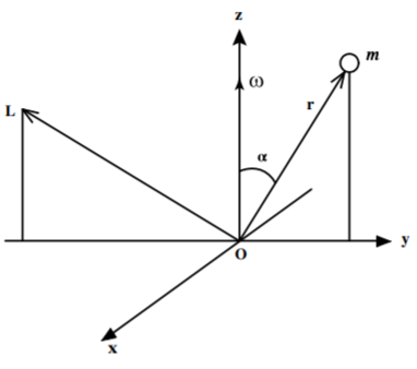
\nonumber \mathbf{L} = \sum_i^n m_i \mathbf{r}_i \times \mathbf{v}_i \sum_i^n m_i \omega_z \begin{pmatrix} -z_ix_i \\ -z_iy_i \\ x_i^2 + y_i^2 \end{pmatrix}

A rigid rotating body comprising a single mass m attached by a massless rod at a fixed angle \alpha shown at the instant when m happens to lie in the yz plane. As the body rotates about the z− axis the mass m has a velocity and momentum into the page (the negative x direction). Therefore the angu… — Figure 2.12.6:A rigid rotating body comprising a single mass $m$ attached by a massless rod at a fixed angle $\alpha$ shown at the instant when $m$ happens to lie in the $yz$ plane. As the body rotates about the $z$ − axis the mass $m$ has a velocity and momentum into the page (the negative $x$ direction). Therefore the angular momentum ${\bf L = r \times p}$ is in the direction shown which is not parallel to the angular velocity $\omega$ .

That is, the components of the angular momentum are

\tag{2.133} \begin{align} L_x & = & - \bigg ( \sum_i^n m_i z_i x_i \bigg ) \omega_z \equiv I_{xz} \omega_z \\ L_y & = & - \bigg ( \sum_i^n m_i z_i y_i \bigg ) \omega_z \equiv I_{yz} \omega_z \notag \\ L_z & = & - \bigg ( \sum_i^n m_i [ x_i^2 + y_i^2 ] \bigg ) \omega_z \equiv I_{xz} \omega_z \notag \end{align}

Note that the perpendicular distance from the $z$ axis in cylindrical coordinates is $\rho = \sqrt{x_i^2 y_i^2}$ thus the angular momentum $L_z$ about the $z$ axis can be written as

\tag{2.134} L_z = \bigg ( \sum_i^n m_i \rho^2 \bigg ) \omega _z = I _{zz} \omega_z

where 2.134 gives the elementary formula for the moment of inertia $I_{zz} = I_{sym}$ about the $z$ axis given earlier in 2.129. The surprising result is that $L_x$ and $L_y$ are non-zero implying that the total angular momentum vector $\mathbf{L}$ is in general not parallel with $\mathbf{\omega}$ This can be understood by considering the single body $m$ shown in Figure 2.12.6. When the body is in the $y, z$ plane then $x = 0$ and $L_x = 0$ . Thus the angular momentum vector $\mathbf{L}$ has a component along the $−y$ direction as shown which is not parallel with $\omega$ and, since the vectors $\mathbf{ \omega, L, r}_i$ are coplanar, then $\mathbf{L}$ must sweep around the rotation axis $\omega$ to remain coplanar with the body as it rotates about the $\omega$ axis. Instantaneously the velocity of the body $v_i$ is into the plane of the paper and, since $\mathbf{L}_i = m_i\mathbf{r}_i \times \mathbf{v}_i$ , then $\mathbf{L}_i$ is at an angle $(90^\circ − \alpha)$ to the $z$ axis. This implies that a torque must be applied to rotate the angular momentum vector. This explains why your automobile shakes if the rotation axis and symmetry axis are not parallel for one wheel.

The first two moments in 2.133 are called products of inertia of the body designated by the pair of axes involved. Therefore, to avoid confusion, it is necessary to define the diagonal moment, which is called the moment of inertia, by two subscripts as $I_{zz}$ Thus in general, a body can have three moments of inertia about the three axes plus three products of inertia. This group of moments comprise the inertia tensor which will be discussed further in chapter 13. If a body has an axis of symmetry along the $z$ axis then the summations will give $I_{xz} = I_{yz} = 0$ while $I_{zz}$ will be unchanged. That is, for rotation about a symmetry axis the angular momentum and rotation axes are parallel. For any axis along which the angular momentum and angular velocity coincide is called a principal axis of the body.

Example 2.12.6: Merry-go-round

A child of mass m jumps onto the outside edge of a circular merry-go-round of moment of inertia $I$ , and radius $R$ and initial angular velocity $\omega_0$ What is the final angular velocity $\omega _f$ ? If the initial angular momentum is $L_0$ and, assuming the child jumps with zero angular velocity, then the conservation of angular momentum implies that

\begin{align*} L_0 & = & L_f \\ I\omega_0 & = & I_\omega + mv_fR \\ I \frac{v_0}{R} & =& \frac{v_f}{R} ( I + mR^2 ) \end{align*}

That is

\frac{v_f}{v_0} = \frac{\omega_f}{\omega_0} = \frac{I}{I + mR^2}

Note that this is true independent of the details of the acceleration of the initially stationary child.

Example 2.12.7: Cue pushes a billiard ball

Consider a billiard ball of mass $M$ and radius $R$ is pushed by a cue in a direction that passes through the center of gravity such that the ball attains a velocity $v_0$ . The friction coefficient between the table and the ball is $\mu$ . How far does the ball move before the initial slipping motion changes to pure rolling motion?

Figure 2.12.7:Cue pushing a billiard ball horizontally at the height of the centre of rotation of the ball.

Since the direction of the cue force passes through the center of mass of the ball, it contributes zero torque to the ball. Thus the initial angular momentum is zero at $t = 0$ . The friction force $f$ points opposite to the direction of motion and causes a torque $N_s$ about the center of mass in the direction $\hat{s}$

\nonumber \mathbf{N}_s = \mathbf{f} \cdot \mathbf{R} = \mu M g R

Since the moment of inertia about the center of a uniform sphere is $I =\frac{2}{5}MR^2$ then the angular acceleration of the ball is

\nonumber \tag{$\alpha$} \dot{\omega} = \frac{\mu M g R}{I} = \frac{ \mu M g R}{\frac{2}{5} MR ^2} = \frac{5}{2} \frac{\mu g}{R}

Moreover the frictional force causes a deceleration $a_s$ of the linear velocity of the center of mass of

\nonumber \tag{$\alpha$} a_s = - \frac{f}{M} = - \mu g

Integrating $\alpha$ from time zero to t gives

\nonumber \omega = \int_0^t \dot{\omega} dt = \frac{5}{2} \frac{ \mu g}{R} t

The linear velocity of the center of mass at time $t$ is given by integration of equation $\beta$

\nonumber v_s = \int_0^t a_s dt = v_0 - \mu gt

The billiard ball stops sliding and only rolls when $v_s = \omega R$ , that is, when

\nonumber \frac{5}{2} \frac{\mu g }{R} tR = v_0 - \mu gt

That is, when

\nonumber t_{roll} = \frac{2}{7} \frac{v_0}{\mu g}

Thus the ball slips for a distance

\nonumber s = \int_0^{t_{roll}} v_s dt = v_0 t_{roll} - \frac{\mu gt_{roll}^2}{2} = \frac{12}{49} \frac{v_0^2}{\mu g }

Note that if the ball is pushed at a distance h above the center of mass, besides the linear velocity there is an initial angular momentum of

\omega = \frac{M v_0 h }{ \frac{2}{5} MR^2} = \frac{5}{2} \frac{v_o h}{R^2}

For the case $h = \frac{2}{5} R$ then the ball immediately assumes a pure non-slipping roll. For $h < \frac{2}{5} R$ one has $\omega < \frac{v_0}{R}$ while $h > \frac{2}{5} R$ corresponds to $\omega > \frac{v_0}{R}$ . In the latter case the frictional force points forward.

Time dependent forces¶

Many problems involve action in the presence of a time dependent force. There are two extreme cases that are often encountered. One is an impulsive force that acts for a very short time, for example, striking a ball with a bat, or the collision of two cars while the second force is an oscillatory time dependent force. The response to impulsive forces is discussed below whereas the response to oscillatory time dependent forces is discussed in chapter 3.

Translational impulsive forces¶

An impulsive force acts for a very short time relative to the response time of the mechanical system being discussed. In principle the equation of motion can be solved if the complicated time dependence of the force, $F(t)$ is known. However, often it is possible to use the much simpler approach employing the concept of an impulse and the principle of the conservation of linear momentum.

Define the linear impulse to be the first-order time integral of the time-dependent force.

\tag{2.135} \mathbf{P} = \int \mathbf{F} (t) dt

Since $\mathbf{F} (t) = \frac{d\mathbf{p}}{dt}$ then Equation 2.135 gives that

\tag{2.136} \mathbf{P} = \int_0^t \frac{d\mathbf{p}}{dt^\prime}dt^\prime = \int_0^t d\mathbf{p} =\mathbf{p}(t) - \mathbf{p}_0 = \Delta \mathbf{p}

Thus the impulse $\mathbf{P}$ is an unambiguous quantity that equals the change in linear momentum of the object that has been struck which is independent of the details of the time dependence of the impulsive force. Computation of the spatial motion still requires knowledge of $F(t)$ since the 2.136 can be written as

\tag{2.137} \mathbf{v}(t) = \frac{1}{m} \int_0^t \mathbf{F}(t^\prime) dt^\prime + \mathbf{v}_0

Integration gives

\tag{2.138} \mathbf{r}(t) - \mathbf{r}_0 = \mathbf{v}_0 t + \int_0^t \Bigg [ \frac{1}{m} \int_0^{t^{\prime \prime}} \mathbf{F} (t^\prime ) dt^\prime \Bigg ] dt^{\prime \prime }

In general this is complicated. However, for the case of a constant force $\mathbf{F}(t) = \mathbf{F}_0$ , this simplifies to the constant acceleration equation

\tag{2.139} \mathbf{r}(t) - \mathbf{r}_0 = \mathbf{v}_0 t + \frac{1}{2} \frac{\mathbf{F}_0}{m}t^2

where the constant acceleration $\mathbf{a} = \frac{\mathbf{F}_0}{m}$ .

Angular impulsive torques¶

Note that the principle of impulse also applies to angular motion. Define an impulsive torque as the first-order time integral of the time-dependent torque.

\tag{2.140} \mathbf{T} \equiv \int \mathbf{N} (t) dt

Since torque is related to the rate of change of angular momentum

\tag{2.141} \mathbf{N} (t) = \frac{d\mathbf{L}}{dt}

then

\tag{2.142} \mathbf{T} = \int_0^t \frac{d\mathbf{L}}{dt^\prime} dt^\prime = \int_0^t d\mathbf{L} = \mathbf{L}(t) - \mathbf{L}_0 = \Delta \mathbf{L}

Thus the impulsive torque $\mathbf{T}$ equals the change in angular momentum $\Delta \mathbf{L}$ of the struck body.

Example 2.12.8: Center of percussion of a baseball bat

When an impulsive force $P$ strikes a bat of mass $M$ at a distance $\mathbf{s}$ from the center of mass, then both the linear momentum of the center of mass, and angular momenta about the center of mass, of the bat are changed. Assume that the ball strikes the bat with an impulsive force $P = \Delta p ^{ball}$ perpendicular to the symmetry axis of the bat at the strike point $S$ which is a distance $s$ from the center of mass of the bat. The translational impulse given to the bat equals the change in linear momentum of the ball as given by Equation 2.136 coupled with the conservation of linear momentum

\nonumber \mathbf{P} = \Delta\mathbf{p}_{cm}^{bat} = M \Delta\mathbf{v}_{cm}^{bat}

Similarly Equation 2.142 gives that the angular impulse $T$ equals the change in angular momentum about the center of mass to be

\mathbf{T} = s \times \mathbf{P} = \Delta \mathbf{L} = I_{cm} \Delta \omega_{cm}

The above equations give that

\nonumber \begin{align*} \Delta \mathbf{v}_{cm}^{bat} & = & \frac{\mathbf{P}}{M} \\ \Delta \mathbf{\omega} & = & \frac{\mathbf{s} \times \mathbf{P}}{\mathbf{I}_{cm}} \end{align*}

Assume that the bat was stationary prior to the strike, then after the strike the net translational velocity of a point $O$ along the body-fixed symmetry axis of the bat at a distance $y$ from the center of mass, is given by

\nonumber \mathbf{v} (y) = \Delta \mathbf{v}_{cm} + \Delta \omega_{cm} \times \mathbf{y} = \frac{\mathbf{P}}{M} + \frac{1}{I_cm}( ( \mathbf{s} \times \mathbf{P} ) \times y ) = \frac{\mathbf{P}}{M} + \frac{1}{I_{cm}} [ ( \mathbf{s \cdot y ) P - (s \cdot P ) y }]

It is assumed that $P$ and $s$ are perpendicular and thus $\mathbf{s \times P } = 0$ which simplifies the above equation to

\nonumber \mathbf{v} (y) = \Delta \mathbf{v}_{cm} + \Delta \mathbf{\omega}_{cm} \times \mathbf{y} = \frac{\mathbf{P}}{M} \bigg ( 1 + \frac{M ( \mathbf{s \cdot y} )}{I_{cm}} \bigg )

Note that the translational velocity of the location $O$ , along the bat symmetry axis at a distance $y$ from the center of mass, is zero if the bracket equals zero, that is, if

\nonumber \mathbf{s \cdot y} = - \frac{I_{cm}}{M} = - k^2_{cm}

where $k_{cm}$ is called the radius of gyration of the body about the center of mass. Note that when the scalar product $s \cdot y = - \frac{I_{cm}}{M} = -k^2_{cm}$ then there will be no translational motion at the point $O$ . This point on the $y$ axis lies on the opposite side of the center of mass from the strike point $S$ , and is called the center of percussion corresponding to the impulse at the point $S$ . The center of percussion often is referred to as the “sweet spot” for an object corresponding to the impulse at the point $S$ . For a baseball bat the batter holds the bat at the center of percussion so that they do not feel an impulse in their hands when the ball is struck at the point $S$ . This principle is used extensively to design bats for all sports involving striking a ball with a bat, such as, cricket, squash, tennis, etc. as well as weapons such of swords and axes used to decapitate opponents.

Example 2.12.9: Energy transfer in charged-particle scattering

Consider a particle of charge $+ e_1$ moving with very high velocity $v_0$ along a straight line that passes a distance $b$ from another charge $+ e_2$ and mass $m$ . Find the energy $Q$ transferred to the mass $m$ during the encounter assuming the force is given by Coulomb’s law. Since the charged particle $e_1$ moves at very high speed it is assumed that charge 2 does not change position during the encounter. Assume that charge 1 moves along the $−y$ axis through the origin while charge 2 is located on the $x$ axis at $x = b$ . Let us consider the impulse given to charge 2 during the encounter. By symmetry the $y$ component must cancel while the $x$ component is given by

\nonumber dp_x = F_xdt = -\frac{e_1e_2}{4 \pi \epsilon_0r^2} \cos \theta dt = -\frac{e_1e_2}{4 \pi \epsilon_0r^2} \cos \theta \frac{dt}{d \theta}d\theta

But

\nonumber r\dot{\theta} = - v_0 \cos \theta

where

\nonumber \frac{b}{r} = \cos ( \pi - \theta ) = -\cos \theta

Thus

\nonumber dp_x = -\frac{e_1e_2}{4 \pi \epsilon_0 b v_0} \cos \theta d\theta

Integrate from $\frac{\pi}{2} < \theta < \frac{3 \pi}{2}$ gives that the total momentum imparted to $e_2$ is

\nonumber p_x = -\frac{e_1 e_2}{4 \pi \epsilon_0 b v_0} \int_{\frac{\pi}{2}}^{\frac{3 \pi}{2}} \cos \theta d \theta = \frac{e_1 e_2}{2 \pi e_0 b v_0}

Thus the recoil energy of charge 2 is given by

\nonumber E_2 = \frac{p_x ^2}{2m} = \frac{1}{2m} \bigg ( \frac{e_1e_2}{2 \pi e_0 b v_0} \bigg ) ^2

Figure 2.12.9:Charged-particle scattering

2.13: Solution of many-body equations of motion¶

The following are general methods used to solve Newton’s many-body equations of motion for practical problems.

Analytic solution¶

In practical problems one has to solve a set of equations of motion since the forces depend on the location of every body involved. For example one may be dealing with a set of coupled oscillators such as the many components that comprise the suspension system of an automobile. Often the coupled equations of motion comprise a set of coupled second-order differential equations.

The first approach to solve such a system is to try an analytic solution comprising a general solution of the inhomogeneous equation plus one particular solution of the inhomogeneous equation. Another approach is to employ numeric integration using a computer.

Successive approximation¶

When the system of coupled differential equations of motion is too complicated to solve analytically one can use the method of successive approximation. The differential equations are transformed to integral equations. Then one starts with some initial conditions to make a first order estimate of the functions. The functions determined by this first order estimate then are used in a second iteration and this is repeated until the solution converges.

An example of this approach is when making Hartree-Foch calculations of the electron distributions in an atom. The first order calculation uses the electron distributions predicted by the one-electron model of the atom. This result then is used to compute the influence of the electron charge distribution around the nucleus on the charge distribution of the atom for a second iteration etc.

Perturbation method¶

The perturbation technique can be applied if the force separates into two parts $F = F_1 + F_2$ where $F_1 > > F_2$ and the solution is known for the dominant $F_1$ part of the force. Then the correction to this solution due to addition of the perturbation $F_2$ usually is easier to evaluate. As an example, consider that one of the Space Shuttle thrusters fires. In principle one has all the gravitational forces acting plus the thrust force of the thruster. The perturbation approach is to assume that the trajectory of the Space Shuttle in the earth’s gravitational field is known. Then the perturbation to this motion due to the very small thrust, produced by the thruster, is evaluated as a small correction to the motion in the Earth’s gravitational field. This perturbation technique is used extensively in physics, especially in quantum physics. An example from my own research is scattering of a $1 GeV \ ^{208}$ Pb ion in the Coulomb field of a $^{197}$ Au nucleus. The trajectory for elastic scattering is simple to calculate since neither nucleus is excited and thus the total energy and momenta are conserved. However, usually one of these nuclei will be internally excited by the electromagnetic interaction. This is called Coulomb excitation. The effect of the Coulomb excitation usually can be treated as a perturbation by assuming that the trajectory is given by the elastic scattering solution and then calculate the excitation probability assuming the Coulomb excitation of the nucleus is a small perturbation to the trajectory.

2.14: Newton’s Law of Gravitation¶

Gravitation plays a fundamental role in classical mechanics as well as being an important example of a conservative central $\big ( \frac{1}{r} \big ) ^2$ force. Although you may not be familiar with the following presentation addressing the gravitational field $\mathbf{g}$ , it is assumed that you have met the identical discussion when addressing the electric field $\mathbf{E}$ in electrostatics. The only difference is that mass $m$ replaces charge $e$ and gravitational field $\mathbf{g}$ replaces the electric field $\mathbf{E}$ . Thus this chapter is designed to be a review of the concepts that can be used for study of any conservative inverse-square law central fields.

In 1666 Newton formulated the Theory of Gravitation which he eventually published in the Principia in 1687. Newton’s Law of Gravitation states that each mass particle attracts every other particle in the universe with a force that varies directly as the product of the mass and inversely as the square of the distance between them. That is, the force on a gravitational point mass $m_G$ produced by a mass $M_G$

\tag{2.143} \mathbf{F}_m = -G \frac{m_G M_G}{r^2} \hat{\mathbf{r}}

where $\hat{\mathbf{r}}$ is the unit vector pointing from the gravitational mass $M_G$ to the gravitational mass $m_g$ as shown in Figure 2.14.1. Note that the force is attractive, that is, it points toward the other mass. This is in contrast to the repulsive electrostatic force between two similar charges. Newton’s law was verified by Cavendish using a torsion balance. The experimental value of $G = (6.6726 \pm 0.0008 \times 10^{-11} \ N \times m^2 / kg^2$

The gravitational force between point particles can be extended to finite-sized bodies using the fact that the gravitational force field satisfies the superposition principle, that is, the net force is the vector sum of the individual forces between the component point particles. Thus the force summed over the mass distribution is

\tag{2.144} \mathbf{F} ( \mathbf{r} )_m = - G m_G \sum_{i=1}^n \frac{m_{G_i}}{r_i^2} \hat{\mathbf{r}}_i

where $\mathbf{r}_i$ is the vector from the gravitational mass $m_{G_i}$ to the gravitational mass $m_G$ at the position $\mathbf{r}$ .

For a continuous gravitational mass distribution $\rho_G ( \mathbf{r^\prime} )$ , the net force on the gravitational mass $m_G$ at the location $\mathbf{r}$ can be written as

\tag{2.145} \mathbf{F}_m ( \mathbf{R} ) = -G m_G \int_v \frac{ \rho_G ( \mathbf{r^\prime} )\big ( \mathbf{\hat{r} - \hat{r^\prime} } \big ) }{ ( \mathbf{ \bar{r} - \bar{r^\prime} } ) ^2 } dv^\prime

where $dv^\prime$ is the volume element at the point $\mathbf{r^\prime }$ as illustrated in Figure 2.14.1.

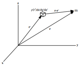
Figure 2.14.1:Gravitational force on mass m due to an infinitessimal volume element of the mass density distribution.

Gravitational and inertial mass¶

Newton’s Laws use the concept of inertial mass $m_I \equiv m$ in relating the force $\mathbf{F}$ to acceleration $\mathbf{a}$

\tag{2.146} \mathbf{F} = m_I \mathbf{a}

and momentum $\mathbf{p}$ to velocity $\mathbf{v}$

\tag{2.147} \mathbf{p} = m_I \mathbf{v}

That is, inertial mass is the constant of proportionality relating the acceleration to the applied force.

The concept of gravitational mass $m_G$ is the constant of proportionality between the gravitational force and the amount of matter. That is, on the surface of the earth, the gravitational force is assumed to be

\tag{2.148} \mathbf{F}_G = m_G \bigg [ -G \sum_{i=1}^n \frac{m_{G_i}}{r_i^2} \hat{\mathbf{r}}_i \bigg ] = m_G \mathbf{g}

where $\mathbf{g}$ is thegravitational field which is a position-dependent force per unit gravitational mass pointing towards the center of the Earth. The gravitational mass is measured when an object is weighed.

Newton’s Law of Gravitation leads to the relation for the gravitational field $\mathbf{g ( r ) }$ at the location $\mathbf{r}$ due to a gravitational mass distribution at the location $\mathbf{r}^\prime$ as given by the integral over the gravitational mass density $\rho_G$

\tag{2.149} \mathbf{g ( r )} = -G \int_V \frac{ \rho_G ( \mathbf{r}^{\prime} ) \big ( \mathbf{\hat{r} - \hat{r}{^\prime} } \big ) }{ ( \mathbf{ \bar{r} - \bar{r}^{\prime} } ) ^2 } d v^\prime

The acceleration of matter in a gravitational field relates the gravitational and inertial masses

\tag{2.150} \mathbf{F} _G = m_G \mathbf{g} = m_I \mathbf{a}

Thus

\tag{2.151} \mathbf{a} = \frac{m_G}{m_I} \mathbf{g}

That is, the acceleration of a body depends on the gravitational strength $g$ and the ratio of the gravitational and inertial masses. It has been shown experimentally that all matter is subject to the same acceleration in vacuum at a given location in a gravitational field. That is, $\frac{m_G }{m_I}$ is a constant common to all materials. Galileo first showed this when he dropped objects from the Tower of Pisa. Modern experiments have shown that this is true to 5 parts in 10¹³.

The exact equivalence of gravitational mass and inertial mass is called the weak principle of equivalence which underlies the General Theory of Relativity as discussed in chapter 17. It is convenient to use the same unit for the gravitational and inertial masses and thus they both can be written in terms of the common mass symbol $m$ .

\tag{2.152} m_I = m_G = m

Therefore the subscripts $G$ and $I$ can be omitted in equations 2.150 and 2.152. Also the local acceleration due to gravity $\mathbf{a}$ can be written as

\tag{2.153} \mathbf{a = g}

The gravitational field $\mathbf{g} \equiv \frac{\mathbf{F}}{m}$ has units of N/kg in the MKS system while the acceleration $\mathbf{a}$ has units $m/s^2$ .

Gravitational potential energy $U$ ¶

Chapter 2.10.2 showed that a conservative field can be expressed in terms of the concept of a potential energy $U( \mathbf{r})$ which depends on position. The potential energy difference $\Delta U_{a \rightarrow b}$ between two points $\mathbf{r}_a$ and $\mathbf{r}_b$ , is the work done moving from $a$ to $b$ against a force $\mathbf{F}$ . That is:

\tag{2.154} \Delta U_{a \rightarrow b} = U( \mathbf{r}_b ) - U( \mathbf{r}_a ) = - \int_{r_a}^{r_b} \mathbf{F} \cdot d\mathbf{l}

In general, this line integral depends on the path taken.

Consider the gravitational field produced by the single point mass $m_1$ . The work done moving a mass $m_0$ from $r_a$ to $r_b$ in this gravitational field can be calculate along an arbitrary path shown in Figure 2.14.2 by assuming Newton’s law of gravitation. Then the force on $m_0$ due to point mass $m_1$ is:

\tag{2.155} \mathbf{F} = - G \frac{m_1 m_0}{r^2} \hat{\mathbf{r}}

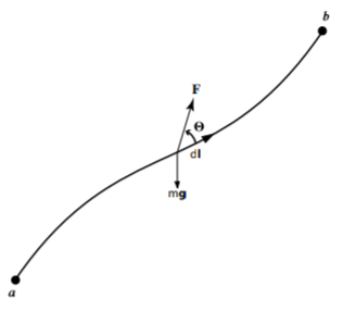
Figure 2.14.2:Work done against a force field moving from a to b.

Expressing $d\mathbf{l}$ in spherical coordinates $d\mathbf{l} = dr \mathbf{\hat{r}} + rd\theta \mathbf{\hat{\theta}} + r \sin \theta d \phi \mathbf{\hat{\phi}}$ gives that the path integral 2.154 from $( r_a \theta_a \phi_a )$ to $( r_b \theta_b \phi_b )$ is

\tag{2.156} \begin{split} \Delta U_{a \rightarrow b} &= - \int_a^b \mathbf{F} \cdot d\mathbf{l} = \int_a^b \big [ G \frac{m_1m_2}{r^2} ( \mathbf{\hat{r} \cdot \widehat{r}} dr + \mathbf{\hat{r}} \cdot \mathbf{\hat{\theta}} d \theta + r \sin \theta \mathbf{\hat{r}} \cdot \hat{\mathbf{\phi}} d \phi ) \big ] = G \int_a^b \frac{m_1m_0}{r^2} \widehat{\mathbf{r}} \cdot \widehat{\mathbf{r}} dr \\ &= -Gm_1m_0 \Big [ \frac{1}{r_b} - \frac{1}{r_a} \Big ] \end{split}

since the scalar product of the unit vectors $\mathbf{ \widehat{r} \cdot \widehat{r}} = 1$ . Note that the second two terms also cancel since $\mathbf{ \widehat{r} \cdot \hat{\theta}} = \mathbf{\hat{r} \cdot \hat{\phi}} = 0$ since the unit vectors are mutually orthogonal. Thus the line integral just depends only on the starting and ending radii and is independent of the angular coordinates or the detailed path taken between $( r_a \theta_a \phi_a )$ and $( r_b \theta_b \phi_b )$ .

Consider the Principle of Superposition for a gravitational field produced by a set of n point masses. The line integral then can be written as

\tag{2.157} \Delta U_{a \rightarrow b }^{net} = -\int_{r_a}^{r_b} \mathbf{F}_{net} \cdot d \mathbf{l} = - \sum_{i=1}^n \int_{r_a}^{r_b} \mathbf{F}_i \cdot d \mathbf{l} = \sum_{i=1}^n \Delta U _{a \rightarrow b}^i

Thus the net potential energy difference is the sum of the contributions from each point mass producing the gravitational force field. Since each component is conservative, then the total potential energy difference also must be conservative. For a conservative force, this line integral is independent of the path taken, it depends only on the starting and ending positions, $\mathbf{r}_a$ and $\mathbf{r}_b$ . That is, the potential energy is a local function dependent only on position. The usefulness of gravitational potential energy is that, since the gravitational force is a conservative force, it is possible to solve many problems in classical mechanics using the fact that the sum of the kinetic energy and potential energy is a constant. Note that the gravitational field is conservative, since the potential energy difference $\Delta_{a \rightarrow b}^{net}$ is independent of the path taken. It is conservative because the force isradial and time independent, it is not due to the $\frac{1}{r^2}$ dependence of the field.

Gravitational potential $\phi$ ¶

Using $\mathbf{F} = m_0\mathbf{g}$ gives that the change in potential energy due to moving a mass $m_0$ from $a$ to $b$ in a gravitational field $\mathbf{g}$ is:

\tag{2.158} \Delta U_{a \rightarrow b}^{net} = - m_0 \int_{r_a}^{r_b} \mathbf{g}_{net}\cdot d\mathbf{l}

Note that the probe mass $m_0$ factors out from the integral. It is convenient to define a new quantity called gravitational potential $\phi$ where

\tag{2.159} \Delta_{a \rightarrow b}^{net} = \frac{\Delta U_{a \rightarrow b}^{net}}{m_0} = -\int_{r_a}^{r_b} \mathbf{g}_{net} \cdot d \mathbf{l}

That is; *gravitational potential difference is the work that must be done, per unit mass, to move from $a$ to $b$ with no change in kinetic energy.*Be careful not to confuse the gravitational potential energy difference $\Delta U _{a \rightarrow b }$ and gravitational potential difference $\Delta \phi_{a \rightarrow b}$ , that is, $\Delta U$ has units of energy, *Joules_,*while $\Delta \phi$ has units of Joules/Kg.

The gravitational potential is a property of the gravitational force field; it is given as minus the line integral of the gravitational field from $a$ to $b$ . The change in gravitational potential energy for moving a mass $m_0$ from $a$ to $b$ is given in terms of gravitational potential by:

\tag{2.160} \Delta U _{a \rightarrow b} ^{net} = m_0 \Delta \phi_{a \rightarrow b }^{net}

Superposition and potential¶

Previously it was shown that the gravitational force is conservative for the superposition of many masses.

To recap, if the gravitational field

\tag{2.161} \mathbf{g}_{net} = \mathbf{g_1 + g_2 + g_3 }

then

\tag{2.162} \phi_{a \rightarrow b}^{net} = - \int_{r_a}^{r_b} \mathbf{g}_{net} \cdot d \mathbf{l} = - \int_{r_a}^{r_b} \mathbf{g}_1 \cdot d \mathbf{l} - \int_{r_a}^{r_b} \mathbf{g}_2 \cdot d \mathbf{l} - \int_{r_a}^{r_b} \mathbf{g}_3 \cdot d \mathbf{l} = \sum_i^n \phi_{a\rightarrow b} ^{i}

Thus gravitational potential is a simple additive scalar field because the Principle of Superposition applies. The gravitational potential, between two points differing by $h$ in height, is $gh$ . Clearly, the greater $g$ or $h$ , the greater the energy released by the gravitational field when dropping a body through the height $h$ . The unit of gravitational potential is the $\frac{Joule}{Kg}$

Potential theory¶

The gravitational force and electrostatic force both obey the inverse square law, for which the field and corresponding potential are related by:

\tag{2.163} \Delta \phi_{a \rightarrow b } = -\int_{r_a}^{r_b} \mathbf{g} \cdot d \mathbf{l}

for an arbitrary infinitessimal element distance $d\mathbf{l}$ the change in electric potential $d \phi$ is

\tag{2.164} d \phi= - \mathbf{g} \cdot d \mathbf{l}

Using cartesian coordinates both $\mathbf{g}$ and $d \mathbf{l}$ can be written as

\tag{2.165} \mathbf{g} = \mathbf{\widehat{i}}g_x + \mathbf{\widehat{j}}g_y + \mathbf{\widehat{k}}g_z \hspace{6cm} d \mathbf{l} = \mathbf{\widehat{i}}dx + \mathbf{\widehat{j}}dy + \mathbf{\widehat{k}}dz

Taking the scalar product gives:

\tag{2.166} d \phi = - \mathbf{g} \cdot d \mathbf{l} = - g_x dx - g_y dy - g_z dz

Differential calculus expresses the change in potential $d \phi$ in terms of partial derivatives by:

\tag{2.167} d \phi = \frac{\partial \phi}{\partial x} dx + \frac{\partial \phi}{\partial y} dy + \frac{\partial \phi}{\partial z} dz

By association, 2.166 and 2.167 imply that

\tag{2.168} \begin{align} g_x = - \frac{\partial \phi}{\partial x} & \hspace{2cm} g_y = - \frac{\partial \phi}{\partial y} & g_z = - \frac{\partial \phi}{\partial z} \end{align}

Thus on each axis, the gravitational field can be written as minus the gradient of the gravitational potential. In three dimensions, the gravitational field is minus the total gradient of potential and the gradient of the scalar function $\phi$ can be written as:

\tag{2.169} \mathbf{g} = - \mathbf{\nabla} \phi

In cartesian coordinates this equals

\tag{2.170} \mathbf{g} = - \Big [ \mathbf{\widehat{i}}\frac{\partial \phi} {\partial x} + \mathbf{\widehat{j}}\frac{\partial \phi}{\partial y} + \mathbf{\widehat{k}}\frac{\partial \phi}{\partial z} \Big ]

Thus the gravitational field is just the gradient of the gravitational potential, which always is perpendicular to the equipotentials. Skiers are familiar with the concept of gravitational equipotentials and the fact that the line of steepest descent, and thus maximum acceleration, is perpendicular to gravitational equipotentials of constant height. The advantage of using potential theory for inverse-square law forces is that scalar potentials replace the more complicated vector forces, which greatly simplifies calculation. Potential theory plays a crucial role for handling both gravitational and electrostatic forces.

Curl of gravitational field¶

It has been shown that the gravitational field is conservative, that is $\Delta U _ {a \rightarrow b}$ is independent of the path taken between $a$ and $b$ Therefore, Equation 2.159 gives that the gravitational potential is independent of the path taken between two points $a$ and $b$ . Consider two possible paths between $a$ and $b$ as shown in Figure 2.14.3. The line integral from $a$ to $b$ via route 1 is equal and opposite to the line integral back from $b$ to $a$ via route 2 if the gravitational field is conservative as shown earlier.

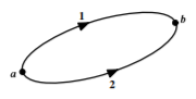
Figure 2.14.3:Circulation of the gravitational field.

A better way of expressing this is that the line integral of the gravitational field is zero around any closed path. Thus the line integral between $a$ and $b$ , via path 1, and returning back to $a$ , via path 2, are equal and opposite. That is, the net line integral for a closed loop is zero.

\tag{2.171} \oint \mathbf{g}_{net} \cdot d \mathbf{l} = 0

which is a measure of the circulation of the gravitational field. The fact that the circulation equals zero corresponds to the statement that the gravitational field is radial for a point mass.

Stokes Theorem, discussed in appendix 19.8.3, states that

\tag{2.172} \oint_C \mathbf{F} \cdot d \mathbf{l} = \int_{\substack{Area \\ bounded \\ by \\ C }} ( \mathbf{\nabla} \times \mathbf{F} ) \cdot d \mathbf{S}

Thus the zero circulation of the gravitational field can be rewritten as

\tag{2.173} \oint_C \mathbf{g} \cdot d \mathbf{l} = \int_{\substack{Area \\ bounded \\ by \\ C }} ( \mathbf{\nabla} \times \mathbf{g} ) \cdot d \mathbf{S} = 0

Since this is independent of the shape of the perimeter $C$ , therefore

\tag{2.174} \mathbf{\nabla} \times \mathbf{g} = 0

That is, the gravitational field is a curl-free field.

A property of any curl-free field is that it can be expressed as the gradient of a scalar potential $\phi$ since

\tag{2.175} \nabla \times \nabla \phi = 0

Therefore, the curl-free gravitational field can be related to a scalar potential $\phi$ as

\tag{2.176} \mathbf{g} = - \mathbf{ \nabla} \phi

Thus $\phi$ is consistent with the above definition of gravitational potential $\phi$ in that the scalar product

\tag{2.177} \Delta \phi_{a \rightarrow b} = - \int_a^b \mathbf{g}_{net} \cdot d \mathbf{l} = \int_a^b ( \mathbf{\nabla} \phi ) \cdot d \mathbf{l} = \int_A^b \sum_i \frac{\partial \phi}{\partial x_i}dx_i = \int_a^b d \phi

An identical relation between the electric field and electric potential applies for the inverse-square law electrostatic field.

Reference potentials¶

Note that only differencesin potential energy, $U$ , and gravitational potential, $\phi$ , are meaningful, the absolute values depend on some arbitrarily chosen reference. However, often it is useful to measure gravitational potential with respect to a particular arbitrarily chosen reference point $\phi_a$ such as to sea level. Aircraft pilots are required to set their altimeters to read with respect to sea level rather than their departure airport. This ensures that aircraft leaving from say both Rochester, $559^\prime$ $msl$ and Denver $5000^\prime$ $msl$ , have their altimeters set to a common reference to ensure that they do not collide. The gravitational force is the gradient of the gravitational field which only depends on differences in potential, and thus is independent of any constant reference.

Gravitational potential due to continuous distributions of charge¶

Suppose mass is distributed over a volume $v$ with a density $\rho$ at any point within the volume. the gravitational potential at any field point $p$ due to an element of mass $dm = \rho v$ at the point $p^\prime$ is given by:

\tag{2.178} \Delta \phi_{\infty \rightarrow p} = -G \int_v \frac{ \rho ( p^\prime ) dv^\prime }{r_{p^\prime p } }

This integral is over a scalar quantity. Since gravitational potential $\phi$ is a scalar quantity, it is easier to compute than is the vector gravitational field $\mathbf{g}$ . If the scalar potential field is known, then the gravitational field is derived by taking the gradient of the gravitational potential.

Gauss’s Law for Gravitation¶

The flux $\Phi$ of the gravitational field $\mathbf{g}$ through a surface $S$ *,*as shown in Figure 2.14.4 is defined as

\tag{2.179} \Phi \equiv \int_S \mathbf{g} \cdot d \mathbf{S}

Note that there are two possible perpendicular directions that could be chosen for the surface vector $d \mathbf{S}$ . Using Newton’s law of gravitation for a point mass $m$ the flux through the surface $S$ is

\tag{2.180} \Phi = - Gm \int_S \frac{\widehat{\mathbf{r}} \cdot d \mathbf{S}}{r^2}

Note that the solid angle subtended by the surface $dS$ at an angle $\theta$ to the normal from the point mass is given by

\tag{2.181} d \Omega = \frac{ \cos \theta dS}{r^2} = \frac{\widehat{\mathbf{r}} \cdot d \mathbf{S}}{r^2}

Thus the net gravitational flux equals

\tag{2.182} \Phi = - Gm \int_S d \Omega

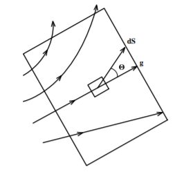
Figure 2.14.4:Flux of the gravitational field through an infinitessimal surface element dS.

Consider a closed surface where the direction of the surface vector $d \mathbf{S}$ is defined as outwards. The net flux out of this closed surface is given by

\tag{2.183} \Phi = - Gm \oint_S \frac{\widehat{\mathbf{r}} \cdot d \mathbf{S}}{r^2} = - Gm \oint_S d \Omega = - Gm 4 \pi

This is independent of where the point mass lies within the closed surface or on the shape of the closed surface. Note that the solid angle subtended is zero if the point mass lies outside the closed surface. Thus the flux is as given by Equation 2.183 if the mass is enclosed by the closed surface, while it is zero if the mass is outside of the closed surface.

Since the flux for a point mass is independent of the location of the mass within the volume enclosed by the closed surface, and using the principle of superposition for the gravitational field, then for n enclosed point masses the net flux is

\tag{2.184} \Phi \equiv \int_S \mathbf{G} \cdot d \mathbf{S} = - 4 \pi G \sum_i^n m_i

This can be extended to continuous mass distributions, with local mass density $\rho$ , giving that the net flux

\tag{2.185} \Phi \equiv \int_S \mathbf{g} \cdot d \mathbf{S} = -4 \pi G \int_{\substack{enclosed \\ volume}} \rho dv

Gauss’s Divergence Theorem was given in appendix 19.8.2 as

\tag{2.186} \Phi = \oint_S \mathbf{F} \cdot d \mathbf{S} = \int_{\substack{enclosed \\ volume}} \mathbf{\nabla} \cdot \mathbf{F} dv

Applying the Divergence Theorem to Gauss’s law gives that

\nonumber \Phi = \oint_s \mathbf{g} \cdot d \mathbf{S} = \int_{\substack{enclosed \\ volume}} \mathbf{\nabla} \cdot \mathbf{g} dv = - 4 \pi G \int_{\substack{enclosed \\ volume}} \rho dv

\tag{2.187} \int_{\substack{enclosed \\ volume}} [ \mathbf{\nabla} \cdot \mathbf{g} + 4 \pi G \rho ] dv = 0

This is true independent of the shape of the surface, thus the divergence of the gravitational field

\tag{2.188} \mathbf{\nabla} \cdot \mathbf{g} = -4 \pi G \rho

This is a statement that the gravitational field of a point mass has a $\frac{1}{r^2}$ dependence.

Using the fact that the gravitational field is conservative, this can be expressed as the gradient of the gravitational potential $\phi$ ,

\tag{2.189} \mathbf{g} = - \mathbf{\nabla} \phi

and Gauss’s law, then becomes

\tag{2.190} \mathbf{\nabla} \cdot \mathbf{\nabla} \phi = 4 \pi G \rho

which also can be written as Poisson’s equation

\tag{2.191} \nabla^2 \phi = 4 \pi G \rho

Knowing the mass distribution $\rho$ allows determination of the potential by solving Poisson’s equation. A special case that often is encountered is when the mass distribution is zero in a given region. Then the potential for this region can be determined by solving Laplace’s equation with known boundary conditions.

\tag{2.192} \nabla^2 \phi = 0

For example, Laplace’s equation applies in the free space between the masses. It is used extensively in electrostatics to compute the electric potential between charged conductors which themselves are equipotentials.

Condensed forms of Newton’s Law of Gravitation¶

The above discussion has resulted in several alternative expressions of Newton’s Law of Gravitation that will be summarized here. The most direct statement of Newton’s law is

\tag{2.193} \mathbf{g ( r ) } = -G \int_V \frac{\rho ( \mathbf{r}^\prime ) \Big ( \mathbf{ \widehat{r} - \widehat{r}} \Big ) }{ ( \mathbf{r} - \mathbf{r}^\prime ) ^2} dv^\prime

An elegant way to express Newton’s Law of Gravitation is in terms of the flux and circulation of the gravitational field. That is

Flux:

\tag{2.194} \Phi \equiv \int_S \mathbf{g} \cdot d \mathbf{S} = - 4\pi G \int_{\substack{enclosed \\ volume}} \rho dv

Circulation:

\tag{2.195} \oint \mathbf{g}_{net} \cdot d \mathbf{l} = 0

The flux and circulation are better expressed in terms of the vector differential concepts of divergence and curl.

Divergence:

\tag{2.196} \mathbf{\nabla} \cdot \mathbf{g} = -4 \pi G \rho

Curl:

\tag{2.197} \mathbf{\nabla} \times \mathbf{g} = 0

Remember that the flux and divergence of the gravitational field are statements that the field between point masses has a $\frac{1}{r^2}$ dependence. The circulation and curl are statements that the field between point masses is radial.

Because the gravitational field is conservative it is possible to use the concept of the scalar potential field $\phi$ . This concept is especially useful for solving some problems since the gravitational potential can be evaluated using the scalar integral

\tag{2.198} \Delta \phi_{\infty \rightarrow p} = - G \int_v \frac{\rho ( \rho^\prime ) d v^\prime}{r_{p^\prime p}}

An alternate approach is to solve Poisson’s equation if the boundary values and mass distributions are known where Poisson’s equation is:

\tag{2.199} \mathbf{\nabla}^2 \phi = 4 \pi G \rho

These alternate expressions of Newton’s law of gravitation can be exploited to solve problems. The method of solution is identical to that used in electrostatics.

Example 2.14.1: gravitational field of a uniform sphere

Consider the simple case of the gravitational field due to a uniform sphere of matter of radius $R$ and mass $M$ . Then the volume mass density

\nonumber \rho = \frac{3M}{4 \pi R^3}

The gravitational field and potential for this uniform sphere of matter can be derived three ways;

a) The field can be evaluated by directly integrating over the volume

\nonumber \mathbf{g ( r ) } = -G \int_S \frac{\rho ( \mathbf{r}^\prime ) \Big ( \mathbf{ \widehat{r} - \widehat{r}} \Big ) }{ ( \mathbf{r} - \mathbf{r}^\prime ) ^2} dV^\prime

b) The potential can be evaluated directly by integration of

\nonumber \Delta \phi_{\infty \rightarrow p} = - G \int_S \frac{\rho ( \rho^\prime ) d V^\prime}{r_{p^\prime p}}

and then

\nonumber \mathbf{g} = - \mathbf{\nabla} \phi

c) The obvious spherical symmetry can be used in conjunction with Gauss’s law to easily solve this problem.

\nonumber \int_S \mathbf{g} \cdot d \mathbf{S} = - 4\pi G \int_{\substack{enclosed \\ volume}} \rho dv

\nonumber \tag{r>R} 4 \pi r^2 g (r) = - 4 \pi GM

That is: for $r > R$

\nonumber \tag{r>R} \mathbf{g} = - G \frac{M}{r^2}\mathbf{\widehat{r}}

Similarly, for $r < R$

\nonumber \tag{r<R} 4 \pi r^2 g ( r) = \frac{4 \pi}{3} r^3 \rho

That is:

\nonumber \tag{r<R} \mathbf{g} = - G \frac{M}{R^3} \mathbf{r}

$Gravitational field \mathbf{g} and gravitational potential \Phi of a uniformly-dense spherical mass distribution of radius R.$

Figure 2.14.5:Gravitational field $\mathbf{g}$ and gravitational potential $\Phi$ of a uniformly-dense spherical mass distribution of radius $R$ .

The field inside the Earth is radial and is proportional to the distance from the center of the Earth. This is Hooke’s Law, and thus ignoring air drag, any body dropped down a hole through the center of the Earth will undergo harmonic oscillations with an angular frequency of $\omega_0 = \sqrt{\frac{GM}{R^3}} = \sqrt{\frac{g}{R}}$ . This gives a period of oscillation of 1.4 hours, which is about the length of a $P235$ lecture in classical mechanics, which may seem like a long time.

Clearly method (c) is much simpler to solve for this case. In general, look for a symmetry that allows identification of a surface upon which the magnitude and direction of the field is constant. For such cases use Gauss’s law. Otherwise use methods (a) or (b) whichever one is easiest to apply. Further examples will not be given here since they are essentially identical to those discussed extensively in electrostatics.

2.E: Review of Newtonian Mechanics (Exercises)¶

Two particles are projected from the same point with velocities $v_1$ and $v_2$ , at elevations $\alpha_1$ and $\alpha_2$ , respectively $(\alpha_1 > \alpha_2)$ . Show that if they are to collide in mid-air the interval between the firings must be
$\frac{2v_1 v_2 \sin (\alpha_1 − \alpha_2)}{g (v_1 \cos \alpha_1 + v_2 \cos \alpha_2)}.\nonumber$
The teeter totter comprises two identical weights which hang on drooping arms attached to a peg as shown. The arrangement is unexpectedly stable and can be spun and rocked with little danger of toppling over.

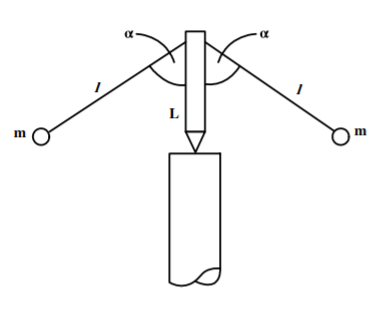
Find an expression for the potential energy of the teeter toy as a function of $\theta$ when the teeter toy is cocked at an angle $\theta$ about the pivot point. For simplicity, consider only rocking motion in the vertical plane.
Determine the equilibrium values(s) of $\theta$ .
Determine whether the equilibrium is stable, unstable, or neutral for the value(s) of $\theta$ found in part (b).
How could you determine the answers to parts (b) and (c) from a graph of the potential energy versus $\theta$ ?
Expand the expression for the potential energy about $\theta = 0$ and determine the frequency of small oscillations.
A particle of mass $m$ is constrained to move on the frictionless inner surface of a cone of half-angle $\alpha$ .
Find the restrictions on the initial conditions such that the particle moves in a circular orbit about the vertical axis.
Determine whether this kind of orbit is stable. A particle of mass $m$ is constrained to move on the frictionless inner surface of a cone of half-angle $\alpha$ , as shown in the figure.
Consider a thin rod of length $L$ and mass $M$ .
Draw gravitational field lines and equipotential lines for the rod. What can you say about the equipotential surfaces of the rod?
Calculate the gravitational potential at a point $P$ that is a distance $r$ from one end of the rod and in a direction perpendicular to the rod.
Calculate the gravitational field at $P$ by direct integration.
Could you have used Gauss’s law to find the gravitational field at $P$ ? Why or why not?
Consider a single particle of mass $m$ .
Determine the position $r$ and velocity $v$ of a particle in spherical coordinates.
Determine the total mechanical energy of the particle in potential $V$ .
Assume the force is conservative. Show that $F = −\nabla V$ . Show that it agrees with Stoke’s theorem.
Show that the angular momentum $L = r \times p$ of the particle is conserved. Hint: $\frac{d}{dt} (A \times B) = A \times \frac{d{\bf B}}{dt} + \frac{d{\bf A}}{dt} \times B$ .
Consider a fluid with density $\rho$ and velocity $v$ in some volume $V$ . The mass current $J = \rho v$ determines the amount of mass exiting the surface per unit time by the integral $\int_S J \cdot dA$ .
Using the divergence theorem, prove the continuity equation, $\nabla \cdot J + \frac{\partial \rho}{\partial t} = 0$
A rocket of initial mass $M$ burns fuel at constant rate $k$ (kilograms per second), producing a constant force $f$ . The total mass of available fuel is $m_o$ . Assume the rocket starts from rest and moves in a fixed direction with no external forces acting on it.
Determine the equation of motion of the rocket.
Determine the final velocity of the rocket.
Determine the displacement of the rocket in time.
Consider a solid hemisphere of radius $a$ . Compute the coordinates of the center of mass relative to the center of the spherical surface used to define the hemisphere.
A 2000 kg Ford was travelling south on Mt. Hope Avenue when it collided with your 1000 kg sports car travelling west on Elmwood Avenue. The two badly-damaged cars became entangled in the collision and leave a skid mark that is 20 meters long in a direction 14° to the west of the original direction of travel of the Excursion. The wealthy Excursion driver hires a high-powered lawyer who accuses you of speeding through the intersection. Use your P235 knowledge, plus the police officer’s report of the recoil direction, the skid length, and knowledge that the coefficient of sliding friction between the tires and road is $\mu = 0.6$ , to deduce the original velocities of both cars. Were either of the cars exceeding the 30 mph speed limit?
A particle of mass $m$ moving in one dimension has potential energy $U(x) = U_0[2(\frac{x}{a})^2 − (\frac{x}{a})^4]$ , where $U_0$ and $a$ are positive constants.
Find the force $F(x)$ that acts on the particle.
Sketch $U(x)$ . Find the positions of stable and unstable equilibrium.
What is the angular frequency $\omega$ of oscillations about the point of stable equilibrium?
What is the minimum speed the particle must have at the origin to escape to infinity?
At $t = 0$ the particle is at the origin and its velocity is positive and equal to the escape velocity. Find $x(t)$ and sketch the result.
Consider a single-stage rocket travelling in a straight line subject to an external force $F^{ext}$ acting along the same line where $v_{ex}$ is the exhaust velocity of the ejected fuel relative to the rocket. Show that the equation of motion is
$m\dot{v} = -\dot{m}v_{ex} + F^{ext} \nonumber$
Specialize to the case of a rocket taking off vertically from rest in a uniform gravitational field $g$ . Assume that the rocket ejects mass at a constant rate of $\dot{m} = −k$ where $k$ is a positive constant. Solve the equation of motion to derive the dependence of velocity on time.
The first couple of minutes of the launch of the Space Shuttle can be described roughly by; initial mass $= 2 \times 10^6$ kg, mass after 2 minutes = $1 \times 10^6$ kg, exhaust speed $v_{ex} = 3000$ m/s and initial velocity is zero. Estimate the velocity of the Space Shuttle after two minutes of flight.
Describe what would happen to a rocket where $\dot{m}v_{ex} < mg$ .
A time independent field $F$ is conservative if $\nabla \times F = 0$ . Use this fact to test if the following fields are conservative, and derive the corresponding potential $U$ .
$F_x = ayz + bx + c, F_y = axz + bz, F_z = axy + by$
$F_x = -ze^{-x}, F_y = \ln z, F_z = e^{-x} + \frac{y}{z}$
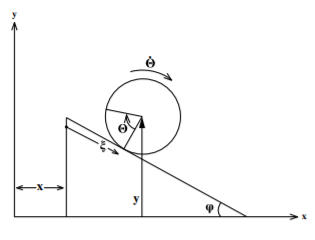
Consider a solid cylinder of mass $m$ and radius $r$ sliding without rolling down the smooth inclined face of a wedge of mass $M$ that is free to slide without friction on a horizontal plane floor. Use the coordinates shown in the figure.
How far has the wedge moved by the time the cylinder has descended from rest a vertical distance $h$ ?
Now suppose that the cylinder is free to roll down the wedge without slipping. How far does the wedge move in this case if the cylinder rolls down a vertical distance $h$ ?
In which case does the cylinder reach the bottom faster? How does this depend on the radius of the cylinder?

If the gravitational field vector is independent of the radial distance within a sphere, find the function describing the mass density $\rho (r)$ of the sphere.

2.S: Newtonian Mechanics (Summary)¶

Newton’s Laws of Motion¶

A cursory review of Newtonian mechanics has been presented. The concept of inertial frames of reference was introduced since Newton’s laws of motion apply only to inertial frames of reference.

Newton’s Law of motion

\tag{2.2.2} \mathbf{F} = \frac{d\mathbf{p}}{dt}

leads to second-order equations of motion which can be difficult to handle for many-body systems.

Solution of Newton’s second-order equations of motion can be simplified using the three first-order integrals coupled with corresponding conservation laws. The first-order time integral for linear momentum is

\tag{2.4.1} \int_1^2 \mathbf{F}_i dt = \int_1^2 \frac{d\mathbf{p}_i}{dt}dt = ( \mathbf{p}_2 - \mathbf{p}_1 ) _i

The first-order time integral for angular momentum is

\tag{2.4.7} \frac{d\mathbf{L}_i}{dt} = \mathbf{r}_i \times \frac{d \mathbf{p}_i}{dt} = \mathbf{N}_i \hspace{4 cm} \int_1^2 \mathbf{N}_i dt = \int_1^2 \frac{d\mathbf{L}_i}{dt}dt = ( \mathbf{L}_2 - \mathbf{L}_1) _i

The first-order spatial integral is related to kinetic energy and the concept of work. That is

\tag{2.4.12} \mathbf{F}_i = \frac{dT_i}{d\mathbf{r}_i} \hspace{4 cm} \int_1^2 \mathbf{F}_i \cdot d\mathbf{r}_i = ( T_2 - T_1) _i

The conditions that lead to conservation of linear and angular momentum and total mechanical energy were discussed for many-body systems. The important class of conservative forces was shown to apply if the position-dependent force do not depend on time or velocity, and if the work done by a force $\int_1^2 \mathbf{F}_i \cdot d \mathbf{r}_i$ is independent of the path taken between the initial and final locations. The total mechanical energy is a constant of motion when the forces are conservative.

It was shown that the concept of center of mass of a many-body or finite sized body separates naturally for all three first-order integrals. The center of mass is that point about which

\tag{Centre of mass definition} \sum_i^n m_i \mathbf{r}_i^\prime = \int \mathbf{r}^\prime \rho dV = 0

where $\mathbf{r}_i^\prime$ is the vector defining the location of mass $m_i$ with respect to the center of mass. The concept of center of mass greatly simplifies the description of the motion of finite-sized bodies and many-body systems by separating out the important internal interactions and corresponding underlying physics, from the trivial overall translational motion of a many-body system..

The Virial theorem states that the time-averaged properties are related by

\tag{2.11.7} \langle T \rangle = - \frac{1}{2} \Bigg \langle \sum_i \mathbf{F}_i \cdot \mathbf{r}_i \Bigg \rangle

It was shown that the Virial theorem is useful for relating the time-averaged kinetic and potential energies, especially for cases involving either linear or inverse-square forces.

Typical examples were presented of application of Newton’s equations of motion to solving systems involving constant, linear, position-dependent, velocity-dependent, and time-dependent forces, to constrained and unconstrained systems, as well as systems with variable mass. Rigid-body rotation about a body-fixed rotation axis also was discussed.

It is important to be cognizant of the following limitations that apply to Newton’s laws of motion:

Newtonian mechanics assumes that all observables are measured to unlimited precision, that is $t, E, \mathbf{P}, \mathbf{r}$ are known exactly. Quantum physics introduces limits to measurement due to wave-particle duality.
The Newtonian view is that time and position are absolute concepts. The Theory of Relativity shows that this is not true. Fortunately for most problems $v < < c$ and thus Newtonian mechanics is an excellent approximation.
Another limitation, to be discussed later, is that it is impractical to solve the equations of motion for many interacting bodies such as molecules in a gas. Then it is necessary to resort to using statistical averages, this approach is called statistical mechanics.

Newton’s work constitutes a theory of motion in the universe that introduces the concept of causality. Causality is that there is a one-to-one correspondence between cause of effect. Each force causes a known effect that can be calculated. Thus the causal universe is pictured by philosophers to be a giant machine whose parts move like clockwork in a predictable and predetermined way according to the laws of nature. This is a deterministic view of nature. There are philosophical problems in that such a deterministic viewpoint appears to be contrary to free will. That is, taken to the extreme it implies that you were predestined to read this book because it is a natural consequence of this mechanical universe!

Newton’s Laws of Gravitation¶

Newton’s Laws of Gravitation and the Laws of Electrostatics are essentially identical since they both involve a central inverse square-law dependence of the forces. The important difference is that the gravitational force is attractive whereas the electrostatic force between identical charges is repulsive. That is, the gravitational constant G is replaced by $\frac{1}{4 \pi \epsilon_0}$ , and the mass density $\rho$ becomes the charge density for the case of electrostatics. As a consequence it is unnecessary to make a detailed study of Newton’s law of gravitation since it is identical to what has already been studied in your accompanying electrostatic courses. Table 2.S.1 summarizes and compares the laws of gravitation and electrostatics. For both gravitation and electrostatics the field is central and conservative and depends as $\frac{1}{r^2} \mathbf{\hat{r}}$ .

The laws of gravitation and electrostatics can be expressed in a more useful form in terms of the flux and circulation of the gravitational field as given either in the vector integral or vector differential forms. The radial independence of the flux, and corresponding divergence, is a statement that the fields are radial and have a $\frac{1}{r^2} \mathbf{\hat{r}}$ dependence. The statement that the circulation, and corresponding curl, are zero is a statement that the fields are radial and conservative.

	Gravitation	Electrostatics
Force field	$\mathbf{g} \equiv \frac{\mathbf{F}_G}{m}$	$\mathbf{E} \equiv \frac{\mathbf{F}_E}{g}$
Density	Mass density $\rho ({\bf r}^\prime )$	Charge density $\rho ({\bf r}^\prime )$
Conservative central field	$\mathbf{g(r)} = -G \int_V \frac{\rho (\mathbf{r}^\prime ) ( \mathbf{\hat{r} - \hat{r^\prime}})}{(\mathbf{r - r^\prime})^2} dv^\prime$	$\mathbf{E(\bar{r})} = \frac{1}{4\pi \epsilon_0} \int_V \frac{\rho (\mathbf{r}^\prime ) ( \mathbf{\hat{r} - \hat{r^\prime}})}{(\mathbf{r - r^\prime})^2} dv^\prime$
Flux	$\Phi \equiv \int_S \mathbf{g} \cdot d\mathbf{S} = -4\pi G \int_{\substack{enclosed \\ volume}} \rho dv$	$\Phi \equiv \int_S \mathbf{E} \cdot d\mathbf{S} = \frac{1}{\epsilon_0} \int_{\substack{enclosed \\ volume}} \rho dv$
Circulation	$\oint\mathbf{g}_{net} \cdot d\mathbf{l} = 0$	$\oint\mathbf{E}_{net} \cdot d\mathbf{l} = 0$
Divergence	$\nabla \cdot \mathbf{g} = -4\pi G \rho$	$\nabla \cdot \mathbf{E} = \frac{1}{\epsilon_0} \rho$
Curl	$\nabla \times \mathbf{g} = 0$	$\nabla \times \mathbf{E} = 0$
Potential	$\Delta \phi_{\infty \rightarrow p} = -G \int_v \frac{\rho (p^\prime ) d v^\prime}{r_{p^\prime p}}$	$\Delta \phi_{\infty \rightarrow p} = \frac{1}{4\pi \epsilon_0} \int_v \frac{\rho (p^\prime ) d v^\prime}{r_{p^\prime p}}$
Poisson’s equation	$\nabla^2 \phi = 4 \pi G \rho$	$\nabla^2 \phi = - \frac{1}{\epsilon_0} \rho$

Both the gravitational and electrostatic central fields are conservative making it possible to use the concept of the scalar potential field $\phi$ . This concept is especially useful for solving some problems since the potential can be evaluated using a scalar integral. An alternate approach is to solve Poisson’s equation if the boundary values and mass distributions are known. The methods of solution of Newton’s law of gravitation are identical to those used in electrostatics and are readily accessible in the literature.

2.1: Introduction to Newtonian Mechanics¶

2.2: Newton’s Laws of motion¶

2.3: Inertial Frames of reference¶

2.4: First-order Integrals in Newtonian mechanics¶

Linear Momentum¶

Angular Momentum¶

Kinetic Energy¶

2.5: Conservation Laws in Classical Mechanics¶

2.6: Motion of finite-sized and many-body systems¶

2.7: Center of Mass of a Many-Body System¶

2.8: Total Linear Momentum of a Many-body System¶

Center-of-mass decomposition¶

Equations of motion¶

2.9: Angular Momentum of a Many-Body System¶

Center-of-mass Decomposition¶

Equations of motion¶

2.10: Work and Kinetic Energy for a Many-Body System¶

Center-of-mass kinetic energy¶

Conservative forces and Potential Energy¶

Total Mechanical Energy¶

Total mechanical energy for conservative systems¶

2.11: Virial Theorem¶

2.12: Applications of Newton’s Equations of Motion¶

Constant Force Problems¶

Linear Restoring Force¶

Position-dependent conservative forces¶

Constrained Motion¶

Velocity Dependent Forces¶

Systems with Variable Mass¶

Rigid-body rotation about a body-fixed rotation axis¶

Rigid-body rotation about a body-fixed symmetry axis¶

Rigid-body rotation about a non-symmetric body-fixed axis¶

Time dependent forces¶

Translational impulsive forces¶

Angular impulsive torques¶

2.13: Solution of many-body equations of motion¶

Analytic solution¶

Successive approximation¶

Perturbation method¶

2.14: Newton’s Law of Gravitation¶

Gravitational and inertial mass¶

Gravitational potential energy UUU¶

Gravitational potential ϕ\phiϕ¶

Superposition and potential¶

Potential theory¶

Curl of gravitational field¶

Reference potentials¶

Gravitational potential due to continuous distributions of charge¶

Gauss’s Law for Gravitation¶

Condensed forms of Newton’s Law of Gravitation¶

2.E: Review of Newtonian Mechanics (Exercises)¶

2.S: Newtonian Mechanics (Summary)¶

Newton’s Laws of Motion¶

Newton’s Laws of Gravitation¶

Gravitational potential energy $U$ ¶

Gravitational potential $\phi$ ¶