Chapter 3 discussed the behavior of a single linearly-damped linear oscillator subject to a harmonic force. No account was taken for the influence of the single oscillator on the driver for the case of forced oscillations. Many systems in nature comprise complicated free or forced oscillations of coupled-oscillator systems. Examples of coupled oscillators are; automobile suspension systems, electronic circuits, electromagnetic fields, musical instruments, atoms bound in a crystal, neural circuits in the brain, networks of pacemaker cells in the heart, etc. Energy can be transferred back and forth between coupled oscillators as the motion evolves. However, it is possible to describe the motion of coupled linear oscillators in terms of a sum over independent normal coordinates, i.e. normal modes, even though the motion may be very complicated. These normal modes are constructed from the original coordinates in such a way that the normal modes are uncoupled. The topic of finding the normal modes of coupled oscillator systems is a ubiquitous problem encountered in all branches of science and engineering. As discussed in chapter 3, oscillatory motion of non-linear systems can be complicated. Fortunately most oscillatory systems are approximately linear when the amplitude of oscillation is small. This discussion assumes that the oscillation amplitudes are sufficiently small to ensure linearity.
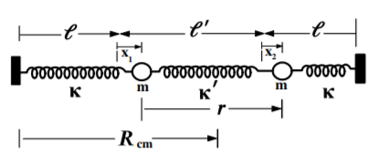
Consider the two-coupled linear oscillator, shown in Figure 14.2.1, which comprises two identical masses each connected to fixed locations by identical springs having a force constant κ. A spring with force constant κ′ couples the two oscillators. The equilibrium lengths of the outer two springs are l while that of the coupling spring is l′. The problem is simplified by restricting the motion to be along the line connecting the masses and assuming fixed endpoints. The small displacements of m1 and m2 are taken to be x1 and x2 with respect to the equilibrium positions l and l+l′ respectively. The restoring force on m1 is −κx1−κ′(x1−x2) while the restoring force on m2 is −κx2−κ′(x2−x1). This coupled double-oscillator system exhibits basic features of coupled linear oscillator systems.
Figure 14.2.1:Two coupled linear oscillators. The equilibrium spring-lengths are l for the outer springs and l′ for the coupling spring. The displacement from the stable locations are given by x1 and x2. The separation between the two masses is r and the location of the center-of-mass is Rcm.
Assuming m1=m2=m, then the equations of motion are
Assume that the motion for these coupled equations is oscillatory with a solution of the form
x1=B1eiωtx2=B2eiωt(14.2)
where the constants B may be complex to take into account both the magnitude and phase. Substituting these possible solutions into the equations of motion gives
The existence of a non-trivial solution of these two simultaneous equations requires that the determinant of the coefficients of B1 and B2 must vanish, that is
∣∣κ+κ′−mω2−κ′−κ′κ+κ′−mω2∣∣=0(14.5)
The expansion of this secular determinant yields
(κ+κ′−mω2)2−κ′2=0(14.6)
Solving for ω gives
ω=mκ+κ′±κ′(14.7)
That is, there are two characteristic frequencies (or eigenfrequencies) for the system
ω1=mκ+2κ′(14.8)
ω2=mκ(14.9)
Since superposition applies for these linear equations, then the general solution can be written as a sum of the terms that account for the two possible values of ω.
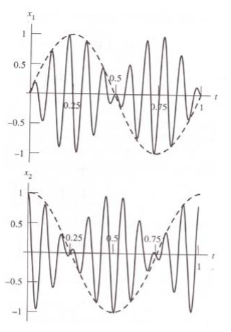
Figure 14.2.2:Displacement of each of two coupled linear harmonic oscillators with κ=4 and κ′=1 in relative units.
Figure 14.2.2 shows the solutions for a case where κ=4 and κ′=1, in arbitrary units, with the initial condition that x2=D, and x1=x˙1=x˙2=0. The two characteristic frequencies are ω1=m6 and ω2=m4. The characteristic beats phenomenon is exhibited where the envelope over one complete cycle of the low frequency encompasses several higher frequency oscillations. That is, the solution is
The energy in the two-coupled oscillators flows back and forth between the coupled oscillators as illustrated in Figure 14.2.2.
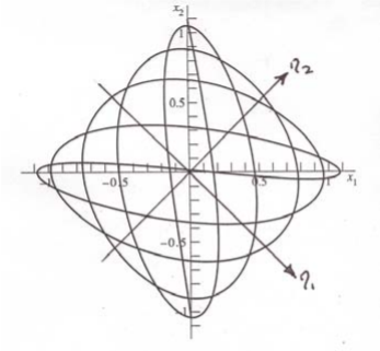
A better understanding of the energy flow occurring between the two coupled oscillators is given by using a (x1,x2) configuration-space plot, shown in Figure 14.3.1. The flow of energy occurring between the two coupled oscillators can be represented by choosing normal-mode coordinates η1 and η2 that are rotated by 45∘ with respect to the spatial coordinates (x1,x2). These normal-mode coordinates (η1,η2) correspond to the two normal modes of the coupled double-oscillator system.
The normal modes of the two-coupled oscillator system are obtained by a transformation to a pair of normal coordinates(η1,η2) that are independent and correspond to the two normal modes. The pair of normal coordinates for this case are
η1≡x1−x2η2≡x1+x2(14.12)
that is
x1=21(η2+η1)x2=21(η2−η1)(14.13)
Substitute these into the equations of motion (14.2.1), gives
where η1 corresponds to angular frequencies ω1, and η2 corresponds to ω2. The two coordinates η1 and η2 are called the normal coordinates and the two solutions are the normal modes with corresponding angular frequencies,ω1 and ω2.
Figure 14.3.1:Motion of two coupled harmonic oscillators in the (x1,x2) spatial configuration space and in terms of the normal modes (η1,η2). Initial conditions are x2=D,x1=x˙1=x˙2=0.
The (η1,η2) axes of the two normal modes correspond to a rotation of 45∘ in configuration space, Figure 14.3.1. The initial conditions chosen correspond to η1=−η2 and thus both modes are excited with equal intensity. Note that there are 5 lobes along the η2 axis versus 4 lobes along the η1 axis reflecting the ratio of the eigenfrequencies ω1 and ω2. Also note that the diamond shape of the motion in the (x1,x2) configuration space illustrates that the extrema amplitudes for x2 are a maximum when x1 is zero, and vice versa. This is equivalent to the statement that the energies in the two modes are coupled with the energy for the first oscillator being a maximum when the energy is a minimum for the second oscillator, and vice versa. By contrast, in the (η1,η2) configuration space, the motion is bounded by a rectangle parallel to the (η1,η2) axes reflecting the fact that the extrema amplitudes, and corresponding energies, for the η1 normal mode are constant and independent of the motion for the η2 normal mode, and vice versa. The decoupling of the two normal modes is best illustrated by considering the case when only one of these two normal modes is excited. For the initial conditions x1(0)=−x2(0), and x˙1(0)=−x˙2(0), then η2(t)=0. That is, only the η1(t) normal mode is excited with frequency ω1 which corresponds to motion confined to the η1 axis of Figure 14.3.1.
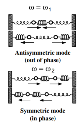
As shown in Figure 14.3.2, η1(t) is the antisymmetric mode in which the two masses oscillate out of phase such as to keep the center of mass of the two masses stationary. For the initial conditions x1(0)=x2(0), and x˙1(0)=x˙2(0), then η1(t)=0, that is, only the η2(t) normal mode is excited. The η2(t) normal mode is the symmetric mode where the two masses oscillate in phase with frequency ω2; it corresponds to motion along the η2 axis. For the symmetric phase, both masses move together leading to a constant extension of the coupling spring. As a result the frequency ω2 of the symmetric mode η2(t) is lower than the frequency ω1 of the asymmetric mode η1(t). That is, the asymmetric mode is stiffer since all three springs provide active restoring forces, compared to the symmetric mode where the coupling spring is uncompressed. In general, for attractive forces the lowest frequency always occurs for the mode with the highest symmetry
Transforming the coordinates into the center of mass of the two oscillating masses elucidates an interesting feature of the normal modes for the two-coupled linear oscillator. As illustrated in Figure (14.2.1), the center-of-mass coordinate for the two mass system is
2Rcm=l+x1+l+l′+x2=2l+l′+η2
while the relative separation distance is
r=(l+l′+x2)−(l+x1)=l′−η1
That is, the two normal modes are
η1=l′−rη2=2Rcm−2l−l′
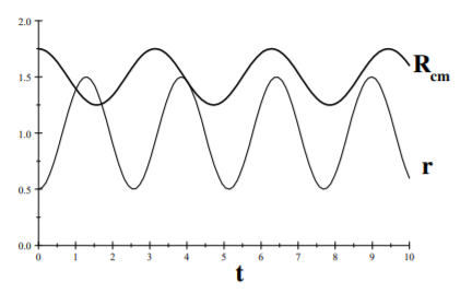
The η1 mode, which has angular frequency ω1=Mκ+2κ′ corresponds to an oscillations of the relative separation r, while the center-of-mass location Rcm is stationary. By contrast, the η2 mode, with angular frequency ω2=Mκ corresponds to an oscillation of the center of mass Rcm with the relative separation r being a constant.
Figure 14.4.1:Time dependence of the center-of-mass Rcm and relative separation r for two coupled linear oscillators assuming spring constants of κ=4M and κ′=M.
Figure 14.4.1 illustrates the decoupled center-of-mass Rcm, and relative motions r for both normal modes of the coupled double-oscillator system. The difference in angular frequencies and amplitudes is readily apparent. It is of interest to consider the special case where the spring constant κ=0 for the two outside springs. Then the angular frequencies are ω1=M2κ′ and ω2=0 for the two normal modes. When κ=0 the η2 mode is a spurious center-of-mass mode since it corresponds to an oscillation with ω2=0 in spite of the fact that there are no forces acting on the center of mass. That is, the center-of-mass momentum must be a constant of motion. This spurious center-of-mass oscillation is a consequence of measuring the displacements (x1,x2) with respect to an arbitrary external reference that is not related to the center of mass of the coupled system. Spurious center-of-mass modes are encountered frequently in many-body coupled oscillator systems such as molecules and nuclei. In such cases it is necessary to project out the center-of-mass motion to eliminate such spurious solutions as will be discussed later.
If one of the two coupled linear oscillator masses is held fixed, then the other free mass will oscillate with a frequency.
ω0=Mκ+κ′(14.18)
The effect of coupling of the two oscillators is to split the degeneracy of the frequency for each mass to
ω1=Mκ+2κ′>ω0=Mκ+κ′>ω2=Mκ(14.19)
Thus the degeneracy is broken, and the two normal modes have frequencies straddling the single-oscillator frequency.
It is interesting to consider the case where the coupling is weak because this situation occurs frequently in nature. The coupling is weak if the coupling constant κ′≪κ. Then
ω1=Mκ+2κ′=Mκ′1+4ε(14.20)
where
ε≡2κκ′≪1(14.21)
Thus
ω1≈Mκ(1+2ε)(14.22)
The natural frequency of a single oscillator was shown to be
ω0≈Mκ+κ′≈Mκ(1+ε)(14.23)
that is
Mκ=ωo(1−ε)(14.24)
Thus the frequencies for the normal modes for weak coupling can be written as
ω1=Mκ(1+2ε)≈ω0(1−ε)(1+2ε)≈ω0(1+ε)(14.25)
while
ω2=Mκ≈ω0(1−ε)(14.26)
That is the two solutions are split equally spaced about the single uncoupled oscillator value given by Equation 14.23. Note that the single uncoupled oscillator frequency ω0 depends on the coupling strength κ′.
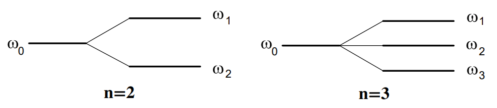
This splitting of the characteristic frequencies is a feature exhibited by many systems of n identical oscillators where half of the frequencies are shifted upwards and half downward. If n is odd, then the central frequency is unshifted as illustrated for the case of n=3. An example of this behavior is the Zeeman effect where the magnetic field couples the atomic motion resulting in a hyperfine splitting of the energy levels of the form illustrated.
Figure 14.5.1:Normal-mode frequencies for n=2 and n=3 weakly-coupled oscillators.
There are myriad examples involving weakly-coupled oscillators applied to musical instruments, physics, and engineering. Weakly coupled oscillators are a dominant theme throughout biology as illustrated by congregations of synchronously flashing fireflies, crickets that chirp in unison, an audience clapping at the end of a performance, networks of pacemaker cells in the heart, insulin-secreting cells in the pancreas, and neural networks in the brain and spinal cord that control rhythmic behaviors such as breathing, walking, and eating. Synchronous motion of a large number of weakly-coupled oscillators often leads to large collective motion of weakly-coupled systems as discussed in chapter 14.12
14.6: General Analytic Theory for Coupled Linear Oscillators
The discussion of a coupled double-oscillator system in Section 14.5 has shown that it is possible to select symmetric and antisymmetric normal modes that are independent and each have characteristic frequencies. The normal coordinates for these two normal modes correspond to linear superpositions of the spatial amplitudes of the two oscillators and can be obtained by a rotation into the appropriate normal coordinate system. Extension of this to systems comprising n coupled linear oscillators, requires development of a general analytic theory, that is capable of finding the normal modes and their eigenvalues and eigenvectors. As illustrated for the double oscillator, the solution of many coupled linear oscillators is a classic eigenvalue problem where one has to rotate to the principal axis system to project out the normal modes. The following discussion presents a general approach to the problem of finding the normal coordinates for a system of n coupled linear oscillators.
Consider a conservative system of n coupled oscillators, described in terms of generalized coordinates qk and t with subscript k=1,2,3,…,n for a system with n degrees of freedom. The coupled oscillators are assumed to have a stable equilibrium with generalized coordinates qk0 at equilibrium. In addition, it is assumed that the oscillation amplitudes are sufficiently small to ensure that the system is linear.
For the equilibrium position qk=qk0, the Lagrange equations must satisfy
q˙k=0q¨k=0(14.27)
Every non-zero term of the form dtd∂q˙k∂L in Lagrange’s equations must contain at least either q˙k or q¨k which are zero at equilibrium; thus all such terms vanish at equilibrium. At equilibrium
In chapter 7.6 it was shown that, in terms of fixed rectangular coordinates, the kinetic energy for N bodies, with n generalized coordinates, is expressed as
T=21α=1∑Ni=1∑3mαx˙α,i2(14.29)
Expressing these in terms of generalized coordinates xα,i=xα,i(qj,t) where j=1,2,...n, then the generalized velocities are given by
x˙α,i=j=1∑n∂qj∂xα,iq˙j+∂t∂xα,i(14.30)
As discussed in chapter 7.6, if the system is scleronomic then the partial derivative
∂t∂xα,i=0(14.31)
Thus the kinetic energy, Equation 14.29, of a scleronomic system can be written as a homogeneous quadratic function of the generalized velocities
T=21j,k∑nTjkq˙jq˙k(14.32)
where the components of the kinetic energy tensor T are
Tjk≡α∑Nmαi∑3∂qj∂xα,i∂qk∂xα,i(14.33)
Note that if the velocities q˙ correspond to translational velocity, then the kinetic energy tensor T corresponds to an effective mass tensor, whereas if the velocities correspond to angular rotational velocities, then the kinetic energy tensor T corresponds to the inertia tensor.
It is possible to make an expansion of the Tjk about the equilibrium values of the form
Only the first-order term will be kept since the second and higher terms are of the same order as the higher order terms ignored in the Taylor expansion of the potential. Thus, at the equilibrium point, assume that (∂qk∂T)0=0 where k=1,2,3,...n.
Make a Taylor expansion about equilibrium for the potential energy, assuming for simplicity that the coordinates have been translated to ensure that qk=0 at equilibrium. This gives
The linear term is zero since (∂qk∂U)0=0 at the equilibrium point, and without loss of generality, the potential can be measured with respect to U0. Assume that the amplitudes are small, then the expansion can be restricted to the quadratic term, corresponding to the simple linear oscillator potential
where the components of the potential energy tensor V are defined as
Vjk≡(∂qj∂qk∂2U′)0(14.39)
Note that the order of differentiation is unimportant and thus the quantity Vjk is symmetric
Vjk=Vkj(14.40)
The motion of the system has been specified for small oscillations around the equilibrium position and it has been shown that U′(q1,q2,...qn) has a minimum value at equilibrium which is taken to be zero for convenience.
where the components of the kinetic energy tensor T and potential energy tensor V are
Tjk≡(α∑Nmαi∑3∂qj∂xα,i∂qk∂xα,i)0(14.43)
Vjk≡(∂qj∂qk∂2U′)0(14.44)
Note that qj and qk may have different units, but all the terms in the summations for both T and U′, have units of energy. The Vjk and Tjk values are evaluated at the equilibrium point, and thus both Vjk and Tjk are n×n arrays of values evaluated at the equilibrium location.
Both the kinetic energy and potential energy terms are products of the coordinates leading to a set of coupled equations that are complicated to solve. The problem is greatly simplified by selecting a set of normal coordinates for which both T and U are diagonal, then the coupling terms disappear. Thus a coordinate transformation must be found that simultaneously diagonalizes Tjk and Vjk in order to obtain a set of normal coordinates.
The kinetic energy Tis only a function of generalized velocitiesq˙k while the conservative potential energy is only a function of the generalized coordinatesqk. Thus the Lagrange equations
∂qk∂L−dtd∂q˙k∂L=0(14.45)
reduce to
∂qk∂U+dtd∂q˙k∂T=0(14.46)
But
∂qk∂U=j∑nVjkqj(14.47)
and
∂q˙k∂T=j∑nTjkq˙j(14.48)
Thus the Lagrange equations reduce to the following set of equations of motion,
j∑n(Vjkqj+Tjkq¨j)=0(14.49)
For each k, where 1≤k≤n, there exists a set of n second-order linear homogeneous differential equations with constant coefficients. Since the system is oscillatory, it is natural to try a solution of the form
qj(t)=ajei(ωt−δ)(14.50)
Assuming that the system is conservative, then this implies that ω is real, since an imaginary term for ω would lead to an exponential damping term. The arbitrary constants are the real amplitude aj and the phase δ. Substitution of this trial solution for each k leads to a set of equations
j∑(Vjk−ω2Tjk)aj=0(14.51)
where the common factor ei(ωt−δ) has been removed. Equation 14.51 corresponds to a set of n linear homogeneous algebraic equations that the aj amplitudes must satisfy for each k. For a non-trivial solution to exist, the determinant of the coefficients must vanish, that is
where the symmetry Vjk=Vkj has been included. This is the standard eigenvalue problem for which the above determinant gives the secular equation or the characteristic equation. It is an equation of degree n in ω2. The n roots of this equation are ωr2 where ωr are the characteristic frequencies or eigenfrequencies of the normal modes.
Substitution of ωr2 into Equation 14.52 determines the ratio a1,r:a2,r:a3,r:...:an,r for this solution which defines the components of the n-dimensional eigenvectorar. That is, solution of the secular equations have determined the eigenvalues and eigenvectors of the n solutions of the coupled-channel system.
The equations of motion ∑j(Vjkqj+Tjkq¨j)=0 are linear equations that satisfy superposition. Thus the most general solution qj(t) can be a superposition of the n eigenvectors ajr, that is
qj(t)=r∑najrei(ωrt−δr)(14.53)
Only the real part of qj(t) is meaningful, that is,
Thus the most general solution of these linear equations involves a sum over the eigenvectors of the system which are cosine functions of the corresponding eigenfrequencies.
It can be shown that the eigenvectors are orthogonal. In addition, the above procedure only determines ratios of amplitudes, thus there is an indeterminacy that can be used to normalize the ajr. Thus the eigenvectors form an orthonormal set. Orthonormality of the eigenfunctions for the rank 3 inertia tensor was illustrated in chapter 13.10.2. Similar arguments apply that allow extending orthonormality to higher rank cases such that for n-body coupled oscillators.
The eigenfunction orthogonality for n coupled oscillators can be proved by writing Equation 14.51 for both the sth root and the rth root. That is,
j∑Vjkaks=ωs2j∑Tjkaks(14.55)
j∑Vjkajr=ωr2j∑Tjkajr(14.56)
Multiply Equation 14.55 by ajr and sum over k. Similarly multiply Equation 14.56 by aks and sum over k. These summations lead to
jk∑Vjkajraks=ωs2jk∑Tjkajraks(14.57)
jk∑Vjkajraks=ωr2jk∑Tjkajraks(14.58)
Note that the left-hand sides of these two equations are identical. Thus taking the difference between these equations gives
(ωr2−ωs2)jk∑Tjkajraks=0(14.59)
Note that if (ωr2−ωs2)=0, that is, assuming that the eigenfrequencies are not degenerate, then to ensure that Equation 14.59 is zero requires that
jk∑Tjkajraks=0r=s(14.60)
This shows that the eigenfunctions are orthogonal. If the eigenfrequencies are degenerate, i.e. ωr2=ωs2, then, with no loss of generality, the axes r and s can be chosen to be orthogonal.
The eigenfunction normalization can be chosen freely since only ratios of the eigenfunction components ajr are determined when ωr is used in Equation 14.51. The kinetic energy, given by Equation 14.32 must be positive, or zero for the case of a static system. That is
T=21j,k∑nTjkq˙jq˙k≥0(14.61)
Use the time derivative of Equation 14.54 to determine q˙r and insert into Equation 14.61 gives that the kinetic energy is
Since the term in the square brackets must be positive, then
j,k∑Tjkajrakr≥0(14.64)
Since this sum must be a positive number, and the magnitude of the amplitudes can be chosen freely, then it is possible to normalize the eigenfunction amplitudes to unity. That is, choose that
j,k∑Tjkajraks=1(14.65)
The orthogonality equation, 14.60 and the normalization Equation 14.65 can be combined into a single orthonormalization equation
j,k∑Tjkajraks=δrs(14.66)
This has shown that the eigenvectors form an orthonormal set.
Since the jth component of the rth eigenvector is ajr, then the rth eigenvector can be written in the form
ar=j∑ajrej(14.67)
where ej are the unit vectors for the generalized coordinates.
The above general solution of the coupled-oscillator problem is best expressed in terms of the normal coordinates which are independent. It is more transparent if the superposition of the normal modes are written in the form
qj(t)=r∑nβrajreiωrt(14.68)
where the complex factor βr includes the arbitrary scale factor to allow for arbitrary amplitudes qj as well as the fact that the amplitudes ajr have been normalized and the phase factor δr has been chosen.
The two-body coupled oscillator is the simplest coupled-oscillator system that illustrates the general features of coupled oscillators. The following four examples involve parallel and series couplings of two linear oscillators or two plane pendula.
The above example illustrates that the general analytic theory for coupled linear oscillators gives the same answer as obtained in chapter 14.2 using Newton’s equations of motion. However, the general analytic theory is a more powerful technique for solving complicated coupled oscillator systems. Thus the general analytic theory will be used for solving all the following coupled oscillator problems.
14.8: Three-body coupled linear oscillator systems
Chapter 14.7 discussed parallel and series arrangements of two coupled oscillators. Extending from two to three coupled linear oscillators introduces interesting new characteristics of coupled oscillator systems. For more than two coupled oscillators, coupled oscillator systems separate into two classifications depending on whether each oscillator is coupled to the remaining n−1 oscillators, or when the coupling is only to the nearest neighbors as illustrated below.
There are many examples of coupled oscillations in atomic and molecular physics most of which involve nearest-neighbor coupling. The following two examples are for molecular coupled oscillators. The triatomic molecule is a typical linearly-coupled molecular oscillator. The benzene molecule is an elementary example of a ring structure coupled oscillator.
Note the following properties of the normal modes and their frequencies.
n=1: Adjacent masses vibrate 180° out of phase, thus each spring has maximal compression or extension, leading to the energy of this normal mode being the highest.
n=2,3: These two solutions are degenerate and correspond to two pairs of masses vibrating out of phase while the third pair of masses are stationary. Thus the energy of this normal mode is slightly lower than the n=1 normal mode. Any combination of these degenerate normal modes are equally good solutions.
n=4,5: From the figure it can be seen that both of these solutions correspond to a center of mass oscillation and thus these modes are spurious.
n=6: This vibrational mode has zero energy corresponding to zero restoring force and all six masses moving uniformly in the same direction. This mode corresponds to the rotation of the benzene molecule about the symmetry axis of the ring which usually is taken into account assuming a separate rotational component.
This classical analog of the benzene molecule is interesting because it simultaneously exhibits degenerate normal modes, spurious center of mass oscillation, and a rotational mode.
## 14.10: Discrete Lattice Chain
Crystalline lattices and linear molecules are important classes of coupled oscillator systems where nearest neighbor interactions dominate. A crystalline lattice comprises thousands of coupled oscillators in a three dimensional matrix with atomic spacing of a few $10^{−10}m$. Even though a full description of the dynamics of crystalline lattices demands a quantal treatment, a classical treatment is of interest since classical mechanics underlies many features of the motion of atoms in a crystalline lattice. The linear discrete lattice chain is the simplest example of many-body coupled oscillator systems that can illuminate the physics underlying a range of interesting phenomena in solid-state physics. As illustrated in example $2.12.1$, the linear approximation usually is applicable for small-amplitude displacements of nearest-neighbor interacting systems which greatly simplifies treatment of the lattice chain. The linear discrete lattice chain involves three independent polarization modes, one longitudinal mode, plus two perpendicular transverse modes. The $3n$ degrees of freedom for the $n$ atoms, on a discrete linear lattice chain, are partitioned with $n$ degrees of freedom for each of the three polarization modes. These three polarization modes each have $n$ normal modes, or $n$ traveling waves, and exhibit quantization, dispersion, and can have a complex wave number.
### Longitudinal Motion
The equations of motion for longitudinal modes of the lattice chain can be derived by considering a linear chain of $n$ identical masses, of mass $m$, separated by a uniform spacing $d$ as shown in [Figure 14.10.1](#fig-14-10-1). Assume that the $n$ masses are coupled by $n + 1$ springs, with spring constant $\kappa$, where both ends of the chain are fixed, that is, the displacements $q_0 = q_{n+1} = 0$ and velocities $\dot{q}_0 = \dot{q}_{n+1} = 0$. The force required to stretch a length $d$ of the chain a longitudinal displacements, $q_{j}$ for mass $j$, is $F_j = \kappa q_j$. Thus the potential energy for stretching the spring for segment $(q_{j−1} − q_j )$ is $U_j = \frac{\kappa}{2} (q_{j-1} - q_j)$. The total potential and kinetic energies are
$$
U = \frac{\kappa}{2} \sum^{n+1}_{j=1} (q_{j-1} - q_j)^2 \tag{14.74} \label{eq-14-74}
$$
$$
T = \frac{1}{2} m \sum^{n}_{j=1} \dot{q}^2_j \tag{14.75} \label{eq-14-75}
$$
:::{figure} ../images/lt-21243-12.10.1.png
:label: fig-14-10-1
:enumerator: 14.10.1
:alt: Portion of a lattice chain of identical masses m connected by identical springs of spring constant \kappa. The displacement of the j^{th} mass from the equilibrium position is q_j assumed to be positive to the right.
Portion of a lattice chain of identical masses $m$ connected by identical springs of spring constant $\kappa$. The displacement of the $j^{th}$ mass from the equilibrium position is $q_j$ assumed to be positive to the right.
:::
Since $\dot{q}_{n+1} = 0$ the kinetic energy and Lagrangian can be extended to $j = {n+1}$, that is, the Lagrangian can be written as
$$
L = \frac{1}{2} \sum^{n+1}_{j=1} \left( m\dot{q}^2_j − \kappa (q_{j−1} − q_j )^2 \right)
$$
Using this Lagrangian in the Lagrange-Euler equations gives the following second-order equation of motion for longitudinal oscillations
$$
\ddot{q}_j = \omega^2_o (q_{j-1} − 2q_j + q_{j+1}) \tag{14.77} \label{eq-14-77}
$$
where $j = 1, 2, ....n$ and where
$$
\omega_o \equiv \sqrt{\frac{\kappa}{m}}
$$
### Transverse motion
:::{figure} ../images/lt-21244-12.10.2.png
:label: fig-14-10-2
:enumerator: 14.10.2
:alt: Transverse motion of a linear discrete lattice chain
Transverse motion of a linear discrete lattice chain
:::
The equations of motion for transverse motion on a linear discrete lattice chain, illustrated in [Figure 14.10.2](#fig-14-10-2), can be derived by considering the displacements $q_j$ of the $i^{th}$ mass for $n$ identical masses, with mass $m$, separated by equal spacings $d$ and assuming that the tension in the string is $r = \left( \frac{\partial U}{\partial x} \right)$. Assuming that the transverse deflections $q_j$ are small, then the $j − 1$ to $j$ spring is stretched to a length
$$
d^{\prime} = \sqrt{d^2 + (q_j − q_{j-1})^2}
$$
Thus the incremental stretching is
$$
\delta d \sim \frac{(q_j − q_{j-1})^2}{2d}
$$
The work done against the tension $\tau$ is $\tau \cdot \delta d$ per segment. Thus the total potential energy is
$$
U = \frac{\tau}{2d} \sum^{n+1}_{j=1} (q_{j-1} − q_j )^2
$$
where $q_0$ and $q_{n+1}$ are identically zero.
The kinetic energy is
$$
T = \frac{1}{2} m\sum^n_{ j=1} \dot{q}^2_j
$$
Since $\dot{q}_{n+1} = 0$, the kinetic energy and Lagrangian summations can be extended to $j = n + 1$, that is
$$
L = \frac{1}{2} \sum^{n+1}_{j=1} \left( m\dot{q}^2_j − \frac{\tau}{d} (q_{j-1} − q_j )^2 \right)
$$
Using this Lagrangian in the Lagrange Euler equations gives the following second-order equation of motion for transverse oscillations
$$
\ddot{q}_j = \omega^2_o (q_{j-1} − 2q_j + q_{j+1}) \tag{14.84} \label{eq-14-84}
$$
where $j = 1, 2, ....n$ and
$$
\omega_o \equiv \sqrt{\frac{\tau}{dm}}
$$
The normal modes for the transverse modes comprise standing waves that satisfy the same boundary conditions as for the longitudinal modes. The $n$ equations of motion for longitudinal motion, Equation [14.77](#eq-14-77), or transverse motion, Equation [14.84](#eq-14-84), are identical in form. The major difference is that $\omega_0$ for the transverse normal modes $\omega_o \equiv \sqrt{\frac{\tau}{dm}}$ differs from that for the longitudinal modes which is $\omega_o \equiv \sqrt{\frac{\kappa}{m}}$. Thus the following discussion of the normal modes on a discrete lattice chain is identical in form for both transverse and longitudinal waves.
### Normal modes
The normal modes of the $n$ equations of motion on the discrete lattice chain, are either longitudinal or transverse standing waves that satisfy the boundary conditions at the extreme ends of the lattice chain. The solutions can be given by assuming that the $n$ identical masses on the chain oscillate with a common frequency $\omega$. Then the displacement amplitude for the $j^{th}$ mass can be written in the form
$$
q_j (t) = a_j e^{i\omega t}
$$
where the amplitude $a_j$ can be complex. Substitution into the preceding $n$ equations of motion, [14.77](#eq-14-77), [14.84](#eq-14-84), yields the following recursion relation
$$
\left( −\omega^2 + 2\omega^2_o \right) a_j− \omega^2_0 (a_{j−1} + a_{j+1})=0 \tag{14.87} \label{eq-14-87}
$$
where $j = 1, 2, ...n$. Note that the boundary conditions, $q_0 = 0$ and $q_{n+1} = 0$ require that $a_o = a_{n+1} = 0$.
The above recursion relation corresponds to a system of $n$ homogeneous algebraic equations with $n$ unknowns $a_1, a_2, ...a_n$. A non-trivial solution is given by setting the determinant of its coefficients equal to zero
$$
\begin{vmatrix} −\omega^2 + 2\omega^2_o & −\omega^2_o & 0 & 0 \\ −\omega^2_o & −\omega^2 + 2\omega^2_o & −\omega^2_o & 0 \\ 0 & −\omega^2_o & −\omega^2 + 2\omega^2_o & −\omega^2_o \\ ..... & .... & ..... & ..... \\ 0 & 0 & −\omega^2_o & −\omega^2 + 2\omega^2_o \end{vmatrix} = 0
$$
This secular determinant corresponds to the special case of nearest neighbor interactions with the kinetic energy tensor $\mathbf{T}$ being diagonal and the potential energy tensor $\mathbf{V}$ involving coupling only to adjacent masses. The secular determinant is of order $n$ and thus determines exactly $n$ eigen frequencies $\omega_r$ for each polarization mode.
For large $n$, the solution of this problem is more efficiently obtained by using a recursion relation approach, rather than solving the above secular determinant. The trick is to assume that the phase differences $\phi_r$ between the motion of adjacent masses all are identical for a given polarization. Then the amplitude for the $j^{th}$ mass for the $r^{th}$ frequency mode $\omega_r$ is of the form
$$
a_{jr} = a_{r} e^{i(j\phi_r−\delta_r)}
$$
Insert the above into the recursion relation [14.87](#eq-14-87) gives
$$
\left( −\omega^2_r + 2\omega^2_o \right) − \omega^2_0 \left[ e^{-i\phi_r} + e^{i\phi_r} \right] = 0
$$
which reduces to
$$
\omega^2_r = 2\omega^2_o − 2\omega^2_o \cos \phi_r = 4\omega^2_o \sin^2 \frac{\phi_r}{2}
$$
that is
$$
\omega_r = 2\omega_o \sin \frac{\phi_r}{2}
$$
where $r = 1, 2, 3, ....n$.
Now it is necessary to determine the phase angle $\phi_r$ which can be done by applying the boundary conditions for standing waves on the lattice chain. These boundary conditions for stationary modes require that the ends of the lattice chain are nodes, that is $a_{o,r} = a_{(n+1),r} = 0$. Using the fact that only the real part of $a_{jr}$ has physical meaning, leads to the amplitude for the $j^{th}$ mass for the $r^{th}$ mode to be
$$
a_{j,r} = a_{r} \cos (j\phi_r − \delta_r)
$$
The boundary condition $a_{0r} = 0$ requires that the phase $\delta_r = \frac{\pi}{2}$. That is
$$
a_{jr} = a_{r} \cos \left( j\phi_r − \frac{\pi }{2} \right) = a_{r} \sin j\phi_r \tag{14.93} \label{eq-14-93}
$$
where $r = 1, 2, ..., n$.
The boundary condition for $j = n+1$, gives
$$
a_{(n+1)r} =0= a_{r} \sin (n+1) \phi_r
$$
Therefore
$$
(n+1) \phi_r = r\pi
$$
where $r = 1, 2, 3, ..., n$. That is
$$
\phi_r = \frac{r\pi}{n+1} = \frac{r\pi d}{ (n+1) d} = \frac{r\pi d}{D} = \frac{k_r d}{2} \tag{14.96} \label{eq-14-96}
$$
where $D = (n+1)d$ is the total length of the discrete lattice chain.
The $n$ eigen frequencies for a given polarization are given by
$$
\omega_r = 2\omega_o \sin \frac{r\pi}{ 2 (n+1)} = 2\omega_o \sin \frac{r\pi d}{2 (n+1) d} = 2\omega_o \sin\frac{ r\pi d}{ 2D} = 2\omega_o \sin \frac{k_rd}{ 2} \tag{14.97} \label{eq-14-97}
$$
where the corresponding wavenumber $k_r$ is given by
$$
k_r = \frac{r\pi }{(n+1) d }= \frac{r\pi}{D} = \frac{2\pi}{ \lambda_r}
$$
This implies that the normal modes are quantized with half-wavelengths $\frac{\lambda_r}{2} = \frac{D}{r}$.
:::{figure} ../images/lt-21246-12.10.3.png
:label: fig-14-10-3
:enumerator: 14.10.3
:alt: Plots of the maximal vibrational amplitudes a_r for the r^{th} frequency sinusoidal mode, versus distance along the chain, for transverse normal modes of a vibrating discrete lattice with n = 5. Only r = 1, 2, 3, 4, 5, are distinct modes because r = 6 is a null mode. Note that the modes with r = …
Plots of the maximal vibrational amplitudes $a_r$ for the $r^{th}$ frequency sinusoidal mode, versus distance along the chain, for transverse normal modes of a vibrating discrete lattice with $n = 5$. Only $r = 1, 2, 3, 4, 5,$ are distinct modes because $r = 6$ is a null mode. Note that the modes with $r = 7, 8, 9, 10, 11, 12,$ shown dashed, duplicate the locations of the mass displacement given by the lower-order modes.
:::
Combining equations [14.96](#eq-14-96) and [14.93](#eq-14-93) gives the maximum amplitudes for the eigenvectors to be
$$
a_{jr} = a_r \sin j \frac{k_r d}{2} \tag{14.99} \label{eq-14-99}
$$
For $n$ independent linear oscillators there are only $n$ independent normal modes, that is, for $r = n+1$ the sine function in Equation [14.97](#eq-14-97) must be zero. Beyond $r = n$ the equations do not describe physically new situations. This is illustrated by [Figure 14.10.3](#fig-14-10-3) which shows the transverse modes of a lattice chain with $n = 5$. There are only $n = 5$ independent normal modes of this system since $r = n +1=6$ corresponds to a null mode with all $q_j (t)=0$. Also note that the solutions for $r>n+1$, shown dashed, replicate the mass locations of modes with $r<n+1$, that is, the modes with $r > 6$ are replicas of the lower-order modes.
Note that $\omega_r$ has a maximum value $\omega_r \leq 2\omega_0$ since the sine function cannot exceed unity. This leads to a maximum frequency $\omega_c = 2\omega_0$, called the cut-off frequency, which occurs when $k_rd = \pi$. That is, the null-mode occurs when $r = n+1$ for which Equation [14.99](#eq-14-99) equals zero. The range of $n$ quantized normal modes that can occur is intuitive. That is, the longest half-wavelength $\frac{\lambda_{\text{max}}}{2} = D = ({n+1})d$ equals the total length of the discrete lattice chain. The shortest half-wavelength $\frac{\lambda_{cut−off}}{2} = d$ is set by the lattice spacing. Thus the discrete wavenumbers of the normal modes, for each polarization, range from $k_1$ to $nk_1$ where $n$ is an integer.
Assuming real $k_r$, the normal coordinate $\eta_r$ and corresponding frequency $\omega_r$ are,
$$
\eta_r = a_{r} e^{i\omega_rt}
$$
Equations [14.97](#eq-14-97) and [14.99](#eq-14-99) give the angular frequency and displacement. Note that superposition applies since this system is linear. Therefore the most general solution for each polarization can be any superposition of the form
$$
q_j (t) = \sum^n_{ r=1 } \eta_r \sin \left[ \frac{r\pi j}{ (n+1)} \right]
$$
### Traveling waves
Traveling waves are equally good solutions of the equations of motion [14.77](#eq-14-77), [14.84](#eq-14-84) as are the normal modes. Traveling waves on the one-dimensional lattice chain will be of the form
$$
q (x, t) = Ce^{i(\omega t \pm kx)} \tag{14.102} \label{eq-14-102}
$$
where the distance along the chain $x = \nu d$, that is, it is quantized in units of the cell spacing $d$, with $\nu$ being an integer. The positive sign in the exponent corresponds to a wave traveling in the $−x$ direction while the negative sign corresponds to a wave traveling in the $+x$ direction. The velocity of a fixed phase of the traveling wave must satisfy that $\omega t \pm kx$ is a constant. This will occur if the *phase velocity* of the wave is given by
$$
v^{phase} = \frac{dx}{dt} = \frac{\omega}{k}
$$
The wave has a frequency $f = \frac{\omega}{ 2\pi}$ and wavelength $\lambda = \frac{2\pi}{k}$, thus the phase velocity $v_{phase} = \frac{\omega}{k} = \lambda f$.
Inserting the traveling wave [14.102](#eq-14-102) into the transverse equation of motion [14.84](#eq-14-84) for the discrete lattice chain gives
$$
−\omega^2q_r = \omega^2_0(e^{−\phi_r} − 2 + e^{\phi_r} )q_r
$$
where $j = 1, 2, ....n$. That is
$$
\omega_r = \pm 2\omega_0 \sin \frac{\phi_r}{2} \tag{14.105} \label{eq-14-105}
$$
The phase $\phi_r$ is determined by the Born-von Karman periodic boundary condition that assumes that the chain is duplicated indefinitely on either side of $k = \pm \frac{\pi}{d}$. Thus, for $n$ discrete masses, $k$ must satisfy the condition that $q_r = q_{r+n}$. That is
$$
e^{ik_rnd} = 1
$$
That is
$$
k_r = \frac{2\pi r}{nd}
$$
Note that the periodic boundary condition gives $n$ discrete modes for wavenumbers between
$$
−\frac{\pi}{d} \leq k_r \leq + \frac{\pi}{d}
$$
where the index
$$
r = −\frac{n}{2}, −\frac{n}{2} + 1, ....., \frac{n}{2} − 1, \frac{n}{2} \nonumber
$$
Thus Equation [14.105](#eq-14-105) becomes
$$
\omega_r = \pm 2\omega_0 \sin \frac{k_r d}{2} \tag{14.109} \label{eq-14-109}
$$
Equation [14.109](#eq-14-109) is a dispersion relation that is identical to Equation [14.97](#eq-14-97) derived during the discussion of the normal modes of the lattice chain. This confirms that the traveling waves on the lattice chain are equally good solutions as the normal standing-wave modes. Clearly, superposition of the standing-wave normal modes can lead to traveling waves and vice versa.
### Dispersion
:::{figure} ../images/lt-21245-12.10.4.png
:label: fig-14-10-4
:enumerator: 14.10.4
:alt: Plot of the dispersion curve (\omega versus k) for a monoatomic linear lattice chain subject to only nearest neighbor interactions. The first Brillouin zone is the segment between −\frac{\pi}{d} \leq k \leq \frac{\pi}{d} which covers all independent solutions.
Plot of the dispersion curve ($\omega$ versus $k$) for a monoatomic linear lattice chain subject to only nearest neighbor interactions. The first Brillouin zone is the segment between $−\frac{\pi}{d} \leq k \leq \frac{\pi}{d}$ which covers all independent solutions.
:::
The lattice chain is an interesting example of a dispersive system in that $\omega_r$ is a function of $k_r$. [Figure 14.10.4](#fig-14-10-4) shows a plot of the dispersion curve ($\omega$ versus $k$) for a monoatomic linear lattice chain subject to only nearest neighbor interactions. Note that $\omega$ depends linearly on $k$ for small $k$ and that $\frac{d\omega}{dk} = 0$ at the boundaries of the first Brillouin zone.
The lattice chain has a phase velocity for the $r^{th}$ wave given by
$$
v^{phase}_r = \frac{\omega_r}{k_r} = \omega_0 d \frac{|\sin \frac{k_r d}{2}|}{ \frac{k_r d}{2}}
$$
while the group velocity is
$$
v^{group}_r = \left(\frac{d\omega}{dk} \right)_r = \omega_0 d \cos \frac{k_r d}{2}
$$
Note that in the limit when $\frac{k_r d}{2} \rightarrow 0$, the phase velocity and group velocity are identical, that is, $v^{phase}_r = v^{group}_r = \omega_0d$.
### Complex wavenumber
The maximum allowed frequency, which is called the cut-off frequency, $\omega_c = 2\omega_0$, occurs when $k_rd = \pi$, that is, $\frac{\lambda}{2} = d$. That is, the minimum half-wavelength equals the spacing $d$ between the discrete masses. At the cut-off frequency, the phase velocity is $v^{phase}_r = \frac{2}{\pi } \omega_0d$ and the group velocity $v^{group}_r = 0$.
It is interesting to note that $\omega_r$ can exceed the cut-off frequency $\omega_c = 2\omega_0$ if $k_r$ is assumed to be complex, that is, if
$$
k_r = \kappa_r − i\Gamma_r
$$
Then
$$
\omega_r = 2\omega_0 \sin \frac{k_r d}{2} = 2\omega_0 \sin \frac{d}{2} (\kappa_r − i\Gamma_r)=2\omega_0 \left( \sin \frac{\kappa_rd}{2} \cosh \frac{\Gamma_rd}{2} − i \cos \frac{\kappa_rd}{2} \sinh \frac{\Gamma_rd }{2} \right)
$$
To ensure that $\omega_r$ is real, the imaginary term must be zero, that is
$$
\cos \frac{\kappa_rd}{2} = 0
$$
Therefore
$$
\sin \frac{\kappa_rd}{2} = 1
$$
that is, $k_r = \frac{\pi}{d}$, and the dispersion relation between $\omega$ and $k$ for $\omega > 2\omega_0$ becomes
$$
\omega_r = 2\omega_0 \cosh \frac{\Gamma_rd}{2}
$$
which increases with $\Gamma$. Thus, when $\omega > \omega_c = 2\omega_0$ then the amplitude of the wave is of the form
$$
q_r (t) = a_r e^{−\Gamma_rx}e^{i(\omega_rt−\kappa_rx)}
$$
which corresponds to a spatially damped oscillatory wave with phase velocity
$$
v^{phase}_r = \frac{\omega_r}{\kappa_r}
$$
and damping factor $\Gamma_r$.
There are many examples in physics where the wavenumber is complex as exhibited by the discrete lattice chain for $\frac{\lambda}{2} \leq d$. Other examples are electromagnetic waves in conductors or plasma (example $3.11.3$), matter waves tunneling through a potential barrier, or standing waves on musical instruments which have a complex wavenumber $k$ due to damping.
This simple toy model of the discrete linear lattice chain has illustrated that classical mechanics explains many features of the many-body nearest-neighbor coupled linear oscillator system, including normal modes, standing and traveling waves, cut-off frequency dispersion, and complex wavenumber. These phenomena feature prominently in applications of the quantal discrete coupled-oscillator system to solid-state physics.
## 14.11: Damped Coupled Linear Oscillators
The discussion of coupled linear oscillators has neglected non-conservative damping forces which always exist to some extent in physical systems. In general, dissipative forces are non linear which greatly complicates solving the equations of motion for such coupled oscillator systems. However, for some systems the dissipative forces depend linearly on velocity which allows use of the Rayleigh dissipation function, described in chapter $10.4$. The most general definition of the Rayleigh dissipation function, $10.4$, was given to be
$$
\mathcal{R} = \frac{1}{2} \sum^n_{i=1} \sum^n_{j=1} c_{ij} \dot{q}_i\dot{q}_j
$$
For this special case, it was shown in chapter $10$ that the Lagrange equations can be written in terms of the Rayleigh dissipation function as
$$
\left\{ \frac{d}{dt} \left( \frac{\partial L}{\partial \dot{q}_j}\right) - \frac{\partial L}{\partial q_j} \right\} + \frac{\partial \mathcal{R}}{\partial \dot{q}_j} = Q_j \tag{14.120} \label{eq-14-120}
$$
where $Q_j$ are generalized forces acting on the system that are not absorbed into the potential $U$. Using equations $(14.6.17)$, $(14.6.18)$, and [14.120](#eq-14-120), allows the equations of motion for damped coupled linear oscillators to be written in a matrix form as
$$
\mathbf{\{T\}} \mathbf{\ddot{q}} + \mathbf{\{C\}} \mathbf{\dot{q}}+ \mathbf{\{V\}} \mathbf{q} = \mathbf{\{Q\}}
$$
where the symmetric matrices $\mathbf{\{T\}}$, $\mathbf{\{C\}}$, and $\mathbf{\{V\}}$ are positive definite for positive definite systems. Rayleigh pointed out that in the special case where the damping matrix $\mathbf{\{C\}}$ is a linear combination of the $\mathbf{\{T\}}$ and $\mathbf{\{V\}}$ matrices, then the matrix $\mathbf{\{C\}}$ is diagonal leading to a separation of the damped system into normal modes. As discussed in chapter 4 many systems in nature are linear for small amplitude oscillations allowing use of the Rayleigh dissipation function which provides an analytic solution. However, in general, except for when $\mathbf{\{C\}}$ is small, this separation into normal modes is not possible for damped systems and the solutions must be obtained numerically.
The following example illustrates approaches used to handle linearly-damped coupled-oscillator systems.
::::{admonition} Example 14.11.1: Two linearly-damped coupled linear oscillators
:class: example
:::{figure} ../images/lt-21247-12.11.1.png
:label: fig-14-11-1
:enumerator: 14.11.1
:alt: Two linearly-damped coupled linear oscillators.
Two linearly-damped coupled linear oscillators.
:::
Consider the two coupled oscillator system shown where the two carts have spring constants $k_1, k_2$ and linear damping constants $c_1c_2$. As discussed in example $14.7.2$, the kinetic energy tensor is given by
$$
T = \frac{1}{2} m_1 \dot{q}^2_1 + \frac{1}{2} m_2 \dot{q}^{2}_{2} \label{eq-14-a}\tag{a}
$$
and the potential energy is given by
$$
U = \frac{1}{2} \left[ k_1q^2_1 + k_2 (q_2 − q_1)^2 \right] \\ = \frac{1}{2} \left[ (k_1 + k_2) q^2_1 − 2k_2q_1q_2 + k_2q_2^2 \right] \label{eq-14-b}\tag{b}
$$
Similarly the Rayleigh dissipation function has the form
$$
\mathcal{R} =\frac{1}{2} \left[ c_1\dot{q}^2_1 + c_2 ( \dot{q}^2_2 − \dot{q}^2_1 )\right] = \frac{1}{2} \left[ (c_1 + c_2) \dot{q}^2_1 − 2c_2\dot{q}_1\dot{q}_2 + c_2\dot{q}^2_2 \right] \label{eq-14-c}\tag{c}
$$
Inserting equations [a](#eq-14-a), [b](#eq-14-b), and [c](#eq-14-c) into Equation [14.120](#eq-14-120) gives the two equations of motion to be
$$
m_1 \ddot{q}_1 + (c_1 + c_2) \dot{q}_1 − c_2\dot{q}_2 + (k_1 + k_2) q_1 − k_2q_2 = 0 \\ m_2 \ddot{q}_2 − c_2\dot{q}_1 + c_2\dot{q}_2 − k_2q_1 + k_2q_2 = 0 \nonumber
$$
When the drag is zero the solution of these two coupled equations can be separated into two independent normal modes of the system as described earlier. Usually it is not possible to separate the motion into decoupled normal modes except for certain cases where the dissipative forces can be described by Rayleigh’s dissipation function.
14.12: Collective Synchronization of Coupled Oscillators
Collective synchronization of coupled oscillators is a multifaceted phenomenon where large ensembles of coupled oscillators, with comparable natural frequencies, self synchronize leading to coherent collective modes of motion. Biological examples include congregations of synchronously flashing fireflies, crickets that chirp in unison, an audience clapping at the end of a performance, networks of pacemaker cells in the heart, insulin-secreting cells in the pancreas, as well as neural networks in the brain and spinal cord that control rhythmic behaviors such as breathing, walking, and eating. Example 14.13 illustrates an application to nuclei.
An ensemble of coupled oscillators will have a frequency distribution with a finite width. It is interesting to elucidate how an ensemble of coupled oscillators, that have a finite width frequency distribution, can self synchronize their motion to a unique common frequency, and how that synchronization is maintained over long time periods. The answers to these issues provide insight into the dynamics of coupled oscillators.
The discussion of coupled oscillators has implicitly assumed n identical undamped linear oscillators that have identical, infinitely-sharp, natural frequencies ωi. In nature typical coupled oscillators can have a finitewidth frequency distribution g(ω) about some average value, due to the natural variability of the oscillator parameters for biological systems, the manufacturing tolerances for mechanical oscillators, or the natural Lorentzian frequency distribution associated with the uncertainty principle that occurs even for atomic clocks where the oscillator frequencies are defined directly by the physical constants. Assume that the ensemble of coupled oscillators has a frequency distribution g(ω) about some average value.
Undamped linear oscillators have elliptical closed-path trajectories in phase space whereas dissipation leads to a spiral attractor unless the system is driven such as to preserve the total energy. As described in chapter 4.4 many systems in nature, especially biological systems, have closed limit cycles in phase space where the energy lost to dissipation is replenished by a driving mechanism. The simplest systems for understanding collective synchronization of coupled oscillators are those that involve closed limit cycles in phase space.
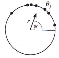
N. Wiener first recognized the ubiquity of collective synchronization in the natural world, but his mathematical approach, based on Fourier integrals, was not suited to this problem. A more fruitful approach was pioneered in 1975 by an undergraduate student A.T. Winfree[Win67] who recognized that the long-time behavior of a large ensemble of limit-cycle oscillators can be characterized in the simplest terms by considering only the phase of closed phase-space trajectories. He assumed that the instantaneous state of an ensemble of oscillators can be represented by points distributed around the circular phase-space diagram shown in Figure 14.12.1. For uncoupled oscillators these points will be distributed randomly around the circle, whereas coupling of the oscillators will result in a spatial correlation of the points. That is, the dynamics of the phases can be visualized as a swarm of points running around the unit circle in the complex plane of the phase space diagram. The complex order parameter of this swarm can be defined to be the magnitude and phase of the centroid of this swarm
reiψ=N1j=1∑Neiθj(14.122)
Figure 14.12.1:Order parameter for weakly-coupled oscillators.
The centroid of the ensemble of points on the phase diagram has a magnitude r, designating the offset of the centroid from the center of the circular phase diagram, and ψ which is the phase of this centroid. A uniform distribution of points around the unit circle will lead to a centroid r=0. Correlated motion leads to a bunching of the points around some phase value leading to a non-zero centroid r and angle ψ. If the swarm acts like a fully-coupled single oscillator then r≈1 with an appropriate phase ψ.
The Kuramoto model[Kur75, Str00] incorporates Winfree’s intuition by mapping the limit cycles onto a simple circular phase diagram and incorporating the long-term dynamics of coupled oscillators in terms of the relative phases for a mean-field system. That is, the angular velocity of the phase ϕ˙i for the ith oscillator is
ϕ˙i=ωi+j=1∑NΓij(ϕj−ϕi)
Figure 14.12.2:Kuramoto model of collective synchronization of coupled oscillators. The left and center plots show the time and coupling strength dependence of the order parameter r. The right plot shows the frequency dependence including coupling (solid line) and without coupling (dashed line).
where i=1,2,,,N. Kuramoto recognized that mean-field coupling was the most tractable system to solve, that is, a system where the coupling is applicable equally to all the oscillators. Moreover, he assumed an equally-weighted, pure sinusoidal coupling for the coupling term Γij(θj−θi) between the coupled oscillators. That is, he assumed
Γij(ϕj−ϕi)=NKsin(ϕj−ϕi)
where K≥0 is the coupling strength, and the factor N1 ensures that the model is well behaved as N→∞. Kuramoto assumed that the frequency distribution g(ω) was unimodular and symmetric about the mean frequency Ω, that is g(Ω+ω)=g(Ω−ω).
This problem can be simplified by exploiting the rotational symmetry and transforming to a frame of reference that is rotating at an angular frequency Ω. That is, use the transformation θi=ϕi−Ωt where θi is measured in the rotating frame. This makes g(ω) unimodular with a symmetric frequency distribution about ω=0. The phase velocity in this rotating frame is
θ˙i=ωi+j=1∑NNKsin(θj−θi)(14.125)
Kuramoto observed that the phase-space distribution can be expressed in terms of the order parameters r,ψ in that Equation 14.122 can be multiplied on both sides by e−iθi to give
for i=1,2,,N. Equation 14.128 reflects the mean-field aspect of the model in that each oscillatorθiis attracted to the phase of the mean fieldψrather than to the phase of another individual oscillator.
Simulations showed that the evolution of the order parameter with coupling strength K is as illustrated in Figure 14.12.2. This simulation shows (1) for all K, when below a certain threshold Kc, the order parameter decays to an incoherent jitter as expected for random scatter of N points. (2) When K>Kc this incoherent state becomes unstable and the order parameter r grows exponentially reflecting the nucleation of small clusters of oscillators that are mutually synchronized. (3) The population of individual oscillators splits into two groups. The oscillators near the center of the distribution lock together in phase at the mean angular frequency Ω and co-rotate with average phase ψ(t), whereas those frequencies lying further from the center continue to rotate independently at their natural frequencies and drift relative to the coherent cluster frequency Ω. As a consequence this mixed state is only partially synchronized as illustrated on the right side of Figure 14.12.2. The synchronized fraction has a δ-function behavior for the frequency distribution which grows in intensity with further increase in K. The unsynchronized component has nearly the original frequency distribution g(ω) except that it is depleted in the region of the locked frequency due to strength absorbed by the δ-function component.
Kuramoto’s toy model nicely illustrates the essential features of the evolution of collective synchronization with coupling strength. It has been applied to the study neuronal synchronization in the brain[Cum07]. The model illustrates that the collective synchronization of coupled oscillators leads to a component that has a single frequency for correlated motion which can be much narrower than the inherent frequency distribution of the ensemble of coupled oscillators.
Two particles, each with mass m, move in one dimension in a region near a local minimum of the potential energy where the potential energy is approximately given by
U=21k(7x12+4x22+4x1x2)
where k is a constant.
Determine the frequencies of oscillation.
Determine the normal coordinates.
What is degeneracy? When does it arise?
The Lagrangian of three coupled oscillators is given by:
n=1∑3[2mx˙n2−2kxn2]+k′(x1x2+x2x3).
Find x2(t) for the following initial conditions (at t=0):
A mechanical analog of the benzene molecule comprises a discrete lattice chain of 6 point masses M connected in a plane hexagonal ring by 6 identical springs each with spring constant κ and length d.
List the wave numbers of the allowed undamped longitudinal standing waves.
Calculate the phase velocity and group velocity for longitudinal traveling waves on the ring.
Determine the time dependence of a longitudinal standing wave for a angular frequency ω=2ωcutoff, that is, twice the cut-off frequency.
Consider a one dimensional, two-mass, three-spring system governed by the matrix A,
A=(4−2−27)
such that Ax=ω2x,
Determine the eigenfrequencies and normal coordinates.
Choose a set of initial conditions such that the system oscillates at its highest eigenfrequency.
Determine the solutions x1(t) and x2(t).
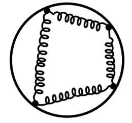
Four identical masses m are connected by four identical springs, spring constant κ, and constrained to move on a frictionless circle of radius b as shown on the left in the figure.
How many normal modes of small oscillation are there?
What are the eigenfrequencies of the small oscillations?
Describe the motion of the four masses for each eigenfrequency.
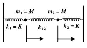
Consider the two identical coupled oscillators given on the right in the figure assuming κ1=κ2=κ. Let both oscillators be linearly damped with a damping constant β. A force F=F0cos(ωt) is applied to mass m1. Write down the pair of coupled differential equations that describe the motion. Obtain a solution by expressing the differential equations in terms of the normal coordinates. Show that the normal coordinates η1 and η2 exhibit resonance peaks at the characteristic frequencies ω1 and ω2 respectively.
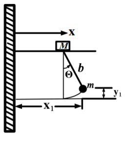
As shown on the left below the mass M moves horizontally along a frictionless rail. A pendulum is hung from M with a weightless rod of length b with a mass m at its end.
This chapter has focused on many—body coupled linear oscillator systems which are a ubiquitous feature in nature. A summary of the main conclusions are the following.
It was shown that coupled linear oscillators exhibit normal modes and normal coordinates that correspond to independent modes of oscillation with characteristic eigenfrequencies ωi.
General analytic theory for coupled linear oscillators
Lagrangian mechanics was used to derive the general analytic procedure for solution of the many-body coupled oscillator problem which reduces to the conventional eigenvalue problem. A summary of the procedure for solving coupled oscillator problems is as follows:.
Choose generalized coordinates qj and evaluate T and U.
T=21j,k∑nTjkq˙jq˙k
and
U′=21j,k∑nVjkqjqk(14.42)
where the components of the T and V tensors are
Tjk≡(α∑Nmαi∑3∂qj∂xα,i∂qk∂xα,i)0(14.43)
and
Vjk≡(∂qj∂qk∂2U)0(14.44)
Determine the eigenvalues ωr using the secular determinant.
The general analytic theory was used to determine the solutions for parallel and series couplings of two and three linear oscillators. The phenomena observed include degenerate and non-degenerate eigenvalues and spurious center-of-mass oscillatory modes. There are two broad classifications for three or more coupled oscillators, that is, either complete coupling of all oscillators, or coupling of the nearest-neighbor oscillators. It is observed that the eigenvalue corresponding to the most coherent motion of the coupled oscillators corresponds to the most collective motion and its eigenvalue is displaced the most in energy from the remaining eigenvalues. For some systems this coherent collective mode corresponded to a center-of-mass motion with no internal excitation of the other modes, while the other eigenvalues corresponded to modes with internal excitation of the oscillators such that the center of mass is stationary. The above procedure has been applied to two classification of coupling, complete coupling of many oscillators, and nearest neighbor coupling. Both degenerate and spurious center-of-mass modes were observed. Strong collective shape degrees of freedom in nuclei are examples of complete coupling due to the weak residual interactions between nucleons in the nucleus. It was seen that, for many coupled oscillators, one coherent state separates from the other states and this coherent state carries the bulk of the collective strength.
Transverse and longitudinal modes of motion on the discrete lattice chain were discussed because of the important role it plays in nature, such as in crystalline lattice structures. Both normal modes and traveling waves were discussed including the phenomena of dispersion and cut-off frequencies. Molecules and the crystalline lattice chains are examples where nearest neighbor coupling is manifest. It was shown that, for the n−oscillator discrete lattice chain, there are only n independent longitudinal modes plus n modes for the two transverse polarizations, and that the angular frequency ωr≤2ω0 that is, a cut-off frequency exists.
It was shown that linearly-damped coupled oscillator systems can be solved analytically using the concept of the Rayleigh dissipation function.
Collective synchronization of coupled oscillators
The Kuramoto schematic phase model was used to illustrate how weak residual forces can cause collective synchronization of the motion of many coupled oscillators. This is applicable to many large coupled systems such as nuclei, molecules, and biological systems.