8. Hamiltonian Mechanics

8.1: Introduction¶

The three major formulations of classical mechanics are

Newtonian mechanics which is the most intuitive vector formulation used in classical mechanics.
Lagrangian mechanics is a powerful algebraic formulation of classical mechanics derived using either d’Alembert’s Principle, or Hamilton’s Principle. The latter states ”A dynamical system follows a path that minimizes the time integral of the difference between the kinetic and potential energies”.
Hamiltonian mechanics has a beautiful superstructure that, like Lagrangian mechanics, is built upon variational calculus, Hamilton’s principle, and Lagrangian mechanics.

Hamiltonian mechanics is introduced at this juncture since it is closely interwoven with Lagrange mechanics. Hamiltonian mechanics plays a fundamental role in modern physics, but the discussion of the important role it plays in modern physics will be deferred until chapters 15 and 18 where applications to modern physics are addressed.

The following important concepts were introduced in chapter 7:

The generalized momentum was defined to be given by

p_{i}\equiv \frac{\partial L(\mathbf{q,\dot{q},}t\mathbf{)}}{\partial \dot{q} _{i}}

Note that, as discussed in chapter 7.2, if the potential is velocity dependent, such as the Lorentz force, then the generalized momentum includes terms in addition to the usual mechanical momentum.

Jacobi’s generalized energy function $h(\mathbf{q,\dot{q}},t)$ was introduced where

h(\mathbf{q,\dot{q}},t)=\sum_{i}^{n}\left( \dot{q}_{i}\frac{\partial L}{ \partial \dot{q}_{i}}\right) -L(\mathbf{q,\dot{q}},t) \tag{8.2}

The Hamiltonian function was defined to be given by expressing the generalized energy function, Equation 8.2, in terms of the generalized momentum. That is, the Hamiltonian $H(\mathbf{q,p},t)$ is expressed as

H\left( \mathbf{q},\mathbf{p},t\right) =\sum_{i}^{n}p_{i}\dot{q}_{i}-L( \mathbf{q},\mathbf{\dot{q}},t) \tag{8.3}

The symbols $\mathbf{q}$ , $\mathbf{p}$ , designate vectors of $n$ generalized coordinates, $\mathbf{q}\equiv (q_{1},q_{2},..q_{n}),$ $\mathbf{p}\equiv (p_{1},p_{2},..p_{n})$ . Equation 8.3 can be written compactly in a symmetric form using the scalar product $\mathbf{p\cdot \dot{q}=} \sum_{i}p_{i}\dot{q}_{i}$ .

H\left( \mathbf{q},\mathbf{p},t\right) +L(\mathbf{q},\mathbf{\dot{q}},t)= \mathbf{p\cdot \dot{q}}

A crucial feature of Hamiltonian mechanics is that the Hamiltonian is expressed as $H\left( \mathbf{q},\mathbf{p},t\right) ,$ that is,it is a function of the $n$ generalized coordinates and their conjugate momenta, which are taken to be independent, plus the independent variable, time. This contrasts with the Lagrangian $L(\mathbf{q},\mathbf{ \dot{q}},t)$ which is a function of the $n$ generalized coordinates $q_{j}$ , and the corresponding velocities $\dot{q}_{j}$ , that is the time derivatives of the coordinates $q_{i}$ , plus the independent variable, time.

8.2: Legendre Transformation between Lagrangian and Hamiltonian mechanics¶

Hamiltonian mechanics can be derived directly from Lagrange mechanics by considering the Legendre transformation between the conjugate variables $\left( \mathbf{q},\mathbf{ \dot{q}},t\right)$ and $\left( \mathbf{q},\mathbf{p},t\right)$ . Such a derivation is of considerable importance in that it shows that Hamiltonian mechanics is based on the same variational principles as those used to derive Lagrangian mechanics; that is d’Alembert’s Principle and Hamilton’s Principle. The general problem of converting Lagrange’s equations into the Hamiltonian form hinges on the inversion of Equation $(8.1.1)$ that defines the generalized momentum $\mathbf{ p.}$ This inversion is simplified by the fact that $(8.1.1)$ is the first partial derivative of the Lagrangian scalar function $L(\mathbf{q, \dot{q},t})$ .

As described in appendix 19.6.4, consider transformations between two functions $F(\mathbf{u,w})$ and $G(\mathbf{v,w),}$ where $\mathbf{u}$ and $\mathbf{v}$ are the active variables related by the functional form

\mathbf{v=\nabla }_{\mathbf{u}}F(\mathbf{u,w}) \tag{8.5}

and where $\mathbf{w}$ designates passive variables. The function $\mathbf{ \nabla }_{\mathbf{u}}F(\mathbf{u,w})$ is the first-order derivative, (gradient) of $F(\mathbf{u,w})$ with respect to the components of the vector $\mathbf{u}$ . The Legendre transform states that the inverse formula can always be written as a first-order derivative

\mathbf{u=\nabla }_{\mathbf{v}}G(\mathbf{v,w})\tag{8.6}

The function $G(\mathbf{v,w})$ is related to $F(\mathbf{u,w})$ by the symmetric relation

G(\mathbf{v,w)+}F\mathbf{(\mathbf{u,w})=u\cdot v}\tag{8.7}

where the scalar product $\mathbf{u\cdot v}=\sum_{i=1}^{N}u_{i}v_{i}$ .

Furthermore the first-order derivatives with respect to all the passive variables $w_{i}$ are related by

\mathbf{\nabla }_{\mathbf{w}}F(\mathbf{u,w)=-\nabla }_{\mathbf{w}}G(\mathbf{ v,w)}\tag{8.8}

The relationship between the functions $F(\mathbf{u,w})$ and $G(\mathbf{v,w})$ is symmetrical and each is said to be the Legendre transform of the other.

The general Legendre transform can be used to relate the Lagrangian and Hamiltonian by identifying the active variables $\mathbf{v}$ ****with $\mathbf{p,}$ and $\mathbf{u}$ with $\mathbf{\dot{q},}$ the passive variable $\mathbf{w}$ with $\mathbf{q,}t$ , and the corresponding functions $F(\mathbf{ u,w)=}L(\mathbf{q,\dot{q},}t)$ and $G(\mathbf{v,w)=}H(\mathbf{q,p,}t )$ . Thus the generalized momentum $(8.1.1)$ corresponds to

\mathbf{p=\nabla }_{\mathbf{\dot{q}}}L(\mathbf{q,\dot{q},}t)\tag{8.9}

where $(\mathbf{q,}t)$ are the passive variables. Then the Legendre transform states that the transformed variable $\mathbf{\dot{q}}$ is given by the relation

\mathbf{\dot{q}=\nabla }_{\mathbf{p}}H(\mathbf{q,p,}t)\tag{8.10}

Since the functions $L(\mathbf{q,\dot{q},}t)$ and $H(\mathbf{q,p,}t )$ are the Legendre transforms of each other, they satisfy the relation

H\left( \mathbf{q},\mathbf{p},t\right) \mathbf{+}L(\mathbf{q},\mathbf{\dot{q} },t)=\mathbf{p\cdot \dot{q}}\tag{8.11}

The function $H\left( \mathbf{q},\mathbf{p},t\right)$ , which is the Legendre transform of the Lagrangian $L(\mathbf{q},\mathbf{\dot{q}},t),$ is called the Hamiltonian function and Equation 8.11 is identical to our original definition of the Hamiltonian given by equation $(8.1.3)$ . The variables $\mathbf{q}$ and $t$ are passive variables thus Equation 8.8 gives that

\mathbf{\nabla }_{\mathbf{q}}L(\mathbf{\dot{q},q,}t\mathbf{)=-\nabla }_{ \mathbf{q}}H(\mathbf{p,q},t)\tag{8.12}

Written in component form Equation 8.12 gives the partial derivative relations $$

\begin{align} \tag{8.13} \frac{\partial L(\mathbf{\dot{q},q,}t)}{\partial q_{i}} &=&-\frac{ \partial H(\mathbf{p,q},t)}{\partial q_{i}} \\ \frac{\partial L(\mathbf{\dot{q},q,}t)}{\partial t} &=&-\frac{ \partial H(\mathbf{p,q},t)}{\partial t}\tag{8.14}\end{align}

Note that equations 8.13 and 8.14 are strictly a result of the Legendre transformation. To complete the transformation from Lagrangian to Hamiltonian mechanics it is necessary to invoke the calculus of variations via the Lagrange-Euler equations. The symmetry of the Legendre transform is illustrated by Equation 8.11.

Equation 7.6.16 gives that the scalar product $\mathbf{p\cdot \dot{q}=} 2T_{2}.$ For scleronomic systems, with velocity independent potentials $U,$ the standard Lagrangian $\,L=T-U$ and $H=2T-T+U=T+U$ . Thus, for this simple case, Equation 8.11 reduces to an identity $H+L=2T$ .

8.3: Hamilton’s Equations of Motion¶

The explicit form of the Legendre transform $(8.2.6)$ gives that the time derivative of the generalized coordinate $q_{j}$ is

\dot{q}_{j}\mathbf{=}\frac{\partial H(\mathbf{q,p,}t)}{\partial p_{j}}\tag{8.15}

The Euler-Lagrange equation $(6.6.1)$ is

\frac{d}{dt}\frac{\partial L}{\partial \dot{q}_{j}}-\frac{\partial L}{ \partial q_{j}}=\sum_{k=1}^{m}\lambda _{k}\frac{\partial g_{k}}{\partial q_{j}}+Q_{j}^{EXC}\tag{8.16}

This gives the corresponding Hamilton equation for the time derivative of $p_{i}$ to be

\frac{d}{dt}\frac{\partial L}{\partial \dot{q}_{j}}=\dot{p}_{j}=\frac{ \partial L}{\partial q_{j}}+\sum_{k=1}^{m}\lambda _{k}\frac{\partial g_{k}}{ \partial q_{j}}+Q_{j}^{EXC}\tag{8.17}

Substitute equation $(8.2.9)$ into Equation 8.17 leads to the second Hamilton equation of motion

\dot{p}_{j}=-\frac{\partial H(\mathbf{q,p,}t)}{\partial q_{j}} +\sum_{k=1}^{m}\lambda _{k}\frac{\partial g_{k}}{\partial q_{j}}+Q_{j}^{EXC}\tag{8.18}

One can explore further the implications of Hamiltonian mechanics by taking the time differential of $(8.1.3)$ giving.

\frac{dH(\mathbf{q,p,}t)}{dt}=\sum_{j}\left( \dot{q}_{j}\frac{dp_{j} }{dt}+p_{j}\frac{d\dot{q}_{j}}{dt}-\frac{\partial L}{\partial q_{j}}\frac{ dq_{j}}{dt}-\frac{\partial L}{\partial \dot{q}_{j}}\frac{d\dot{q}_{j}}{dt} \right) -\frac{\partial L}{\partial t}\tag{8.19}

Inserting the conjugate momenta $p_{i}\equiv \frac{\partial L}{\partial \dot{ q}_{i}}$ and Equation 8.17 into Equation 8.19 results in

\frac{dH(\mathbf{q,p,}t)}{dt}=\sum_{j}\left( \dot{q}_{j}\dot{p} _{j}+p_{j}\frac{d\dot{q}_{j}}{dt}-\left[ \dot{p}_{j}-\sum_{k=1}^{m}\lambda _{k}\frac{\partial g_{k}}{\partial q_{j}}-Q_{j}^{EXC}\right] \dot{q} _{j}-p_{j}\frac{d\dot{q}_{j}}{dt}\right) -\frac{\partial L}{\partial t}\tag{8.20}

The second and fourth terms cancel as well as the $\dot{q}_{j}\dot{p}_{j}$ terms, leaving

\frac{dH(\mathbf{q,p,}t)}{dt}=\sum_{j}\left( \left[ \sum_{k=1}^{m}\lambda _{k}\frac{\partial g_{k}}{\partial q_{j}}+Q_{j}^{EXC} \right] \dot{q}_{j}\right) -\frac{\partial L}{\partial t}\tag{8.21}

This is the generalized energy theorem given by equation $(7.8.1)$ .

The total differential of the Hamiltonian also can be written as

\frac{dH(\mathbf{q,p,}t)}{dt}=\sum_{j}\left( \frac{\partial H}{ \partial p_{j}}\dot{p}_{j}+\frac{\partial H}{\partial q_{j}}\dot{q} _{j}\right) +\frac{\partial H}{\partial t}\tag{8.22}

Use equations 8.15 and 8.18 to substitute for $\frac{\partial H}{ \partial p_{j}}$ and $\frac{\partial H}{\partial q_{j}}$ in Equation 8.22 gives

\frac{dH(\mathbf{q,p,}t)}{dt}=\sum_{j}\left( \left[ \sum_{k=1}^{m}\lambda _{k}\frac{\partial g_{k}}{\partial q_{j}}+Q_{j}^{EXC} \right] \dot{q}_{j}\right) +\frac{\partial H(\mathbf{q,p,}t)}{ \partial t}\tag{8.23}

Note that Equation 8.23 must equal the generalized energy theorem, i.e. Equation 8.21. Therefore,

\frac{\partial H}{\partial t}=-\frac{\partial L}{\partial t}\tag{8.24}

In summary, Hamilton’s equations of motion are given by

\begin{align} \dot{q}_{j} &= \frac{\partial H(\mathbf{q,p,}t)}{\partial p_{j}} \tag{8.25} \\[4pt] \dot{p}_{j} &=-\frac{\partial H(\mathbf{q,p,}t)}{\partial q_{j}}+ \left[ \sum_{k=1}^{m}\lambda _{k}\frac{\partial g_{k}}{\partial q_{j}} +Q_{j}^{EXC}\right] \tag{8.26}\\[4pt] \frac{dH(\mathbf{q,p,}t)}{dt} &= \sum_{j}\left( \left[ \sum_{k=1}^{m}\lambda _{k}\frac{\partial g_{k}}{\partial q_{j}}+Q_{j}^{EXC} \right] \dot{q}_{j}\right) -\frac{\partial L(\mathbf{q,\dot{q},}t)}{ \partial t}\tag{8.27}\end{align}

The symmetry of Hamilton’s equations of motion is illustrated when the Lagrange multiplier and generalized forces are zero. Then

\begin{align} \dot{q}_{j} &= \frac{\partial H(\mathbf{q,p,}t)}{\partial p_{j}} \tag{8.28} \\[4pt] \dot{p}_{j} &= -\frac{\partial H(\mathbf{p,q},t)}{\partial q_{j}} \tag{8.29}\\[4pt] \frac{dH(\mathbf{p,q},t)}{dt} &= \frac{\partial H(\mathbf{p,q},t )}{\partial t}=-\frac{\partial L(\mathbf{\dot{q},q,}t)}{ \partial t}\end{align}\tag{8.30}

This simplified form illustrates the symmetry of Hamilton’s equations of motion. Many books present the Hamiltonian only for this special simplified case where it is holonomic, conservative, and generalized coordinates are used.

Canonical Equations of Motion¶

Hamilton’s equations of motion, summarized in equations 8.25-8.27 use either a minimal set of generalized coordinates, or the Lagrange multiplier terms, to account for holonomic constraints, or generalized forces $Q_{j}^{EXC}$ to account for non-holonomic or other forces. Hamilton’s equations of motion usually are called the canonical equations of motion. Note that the term “canonical” has nothing to do with religion or canon law; the reason for this name has bewildered many generations of students of classical mechanics. The term was introduced by Jacobi in 1837 to designate a simple and fundamental set of conjugate variables and equations. Note the symmetry of Hamilton’s two canonical equations, plus the fact that the canonical variables $p_{k},q_{k}$ are treated as independent canonical variables. The Lagrange mechanics coordinates $(\mathbf{q, \dot{q},}t)$ are replaced by the Hamiltonian mechanics coordinates $(\mathbf{ q,p,}t),$ where the conjugate momenta $\mathbf{p}$ are taken to be independent of the coordinate $\mathbf{q}$ .

Lagrange was the first to derive the canonical equations but he did not recognize them as a basic set of equations of motion. Hamilton derived the canonical equations of motion from his fundamental variational principle, chapter 9.2, and made them the basis for a far-reaching theory of dynamics. Hamilton’s equations give $2s$ first-order differential equations for $p_{k},q_{k}$ for each of the $s=n-m$ degrees of freedom. Lagrange’s equations give $s$ second-order differential equations for the $s$ independent generalized coordinates $q_{k},\dot{q}_{k}.$

It has been shown that $H(\mathbf{p,q},t)$ and $L(\mathbf{\dot{q},q, }t)$ are the Legendre transforms of each other. Although the Lagrangian formulation is ideal for solving numerical problems in classical mechanics, the Hamiltonian formulation provides a better framework for conceptual extensions to other fields of physics since it is written in terms of the fundamental conjugate coordinates, $\mathbf{q,p}$ . The Hamiltonian is used extensively in modern physics, including quantum physics, as discussed in chapters 15 and 18. For example, in quantum mechanics there is a straightforward relation between the classical and quantal representations of momenta; this does not exist for the velocities.

The concept of state space, introduced in chapter 3.3.2, applies naturally to Lagrangian mechanics since $(\dot{q},q)$ are the generalized coordinates used in Lagrangian mechanics. The concept of Phase Space, introduced in chapter 3.3.3, naturally applies to Hamiltonian phase space since $(p,q)$ are the generalized coordinates used in Hamiltonian mechanics.

8.4: Hamiltonian in Different Coordinate Systems¶

Prior to solving problems using Hamiltonian mechanics, it is useful to express the Hamiltonian in cylindrical and spherical coordinates for the special case of conservative forces since these are encountered frequently in physics.

Cylindrical Coordinates $\rho ,z, \phi$ ¶

Consider cylindrical coordinates $\rho ,z,\phi$ . Expressed in Cartesian coordinate

\begin{align*} x &= \rho \cos \phi \\ y &= \rho \sin \phi \notag \\ z &= z \end{align*}

Using appendix table $19.3.3,$ the Lagrangian can be written in cylindrical coordinates as

\begin{align} L &=T-U \\[4pt] &= \frac{m}{2}\left( \dot{\rho}^{2}+\rho ^{2}\dot{\phi}^{2}+\dot{z}^{2}\right) -U(\rho ,z,\phi ) \tag{8.32} \end{align}

The conjugate momenta are

\begin{align} p_{\rho } &= \frac{\partial L}{\partial \dot{\rho}}=m\dot{\rho} \\ p_{\phi } &= \frac{\partial L}{\partial \dot{\phi}}=m\rho ^{2}\dot{\phi} \\ p_{z} &= \frac{\partial L}{\partial \dot{z}}=m\dot{z} \tag{8.35} \end{align}

Assume a conservative force, then $H$ is conserved. Since the transformation from Cartesian to non-rotating generalized cylindrical coordinates is time independent, then $H=E.$ Then using Equations 8.32-8.35 gives the Hamiltonian in cylindrical coordinates to be

\begin{align} H\left( \mathbf{q},\mathbf{p},t\right) &= \sum_{i}p_{i}\dot{q}_{i}-L(\mathbf{ q},\mathbf{\dot{q}},t) \\ &= \left( p_{\rho }\dot{\rho}+p_{\phi }\dot{\phi}+p_{z}\dot{z}\right) -\frac{ m}{2}\left( \overset{.}{\rho }^{2}+\rho ^{2}\overset{.}{\phi }^{2}+\overset{. }{z}^{2}\right) +U(\rho ,z,\phi ) \notag \\ &= \frac{1}{2m}\left( p_{\rho }^{2}+\frac{p_{\phi }^{2}}{\rho ^{2}} +p_{z}^{2}\right) +U(\rho ,z,\phi )\end{align}

The canonical equations of motion in cylindrical coordinates can be written as $$

\begin{align} \dot{p}_{\rho } &= -\frac{\partial H}{\partial \rho }=\frac{p_{\phi }^{2}}{ m\rho ^{3}}-\frac{\partial U}{\partial \rho } \\ \dot{p}_{\phi } &= -\frac{\partial H}{\partial \phi }=-\frac{\partial U}{ \partial \phi } \\ \dot{p}_{z} &= -\frac{\partial H}{\partial z}=-\frac{\partial U}{\partial z} \\ \dot{\rho} &= \frac{\partial H}{\partial p_{\rho }}=\frac{p_{\rho }}{m} \\ \dot{\phi} &= \frac{\partial H}{\partial p_{\phi }}=\frac{p_{\phi }}{m\rho ^{2}} \\ \dot{z} &= \frac{\partial H}{\partial p_{z}}=\frac{p_{z}}{m}\end{align}

Note that if $\phi$ is cyclic, that is $\frac{\partial U}{\partial \phi } =0,$ then the angular momentum about the $z$ axis, $p_{\phi }$ , is a constant of motion. Similarly, if $z$ is cyclic, then $p_{z}$ is a constant of motion.

Spherical coordinates, $r, \theta , \phi$ ¶

Appendix table 19.3.4 shows that the spherical coordinates are related to the cartesian coordinates by

\begin{align} x &= r\sin \theta \cos \phi \\ y &= r\sin \theta \sin \phi \notag \\ z &= r\cos \theta \notag\end{align}

The Lagrangian is

L=T_{i}-U= \frac{m}{2}\left( \dot{r}^{2}+r^{2}\dot{\theta}^{2}+r^{2}\sin ^{2}\theta \dot{\phi}^{2}\right) -U(r\theta \phi )

The conjugate momenta are $$

\begin{align} \tag{8.46} p_{r} &= \frac{\partial L}{\partial \overset{.}{r}}=m\dot{r} \\ p_{\theta } &= \frac{\partial L}{\partial \overset{.}{\theta }}=mr^{2}\dot{ \theta} \\ p_{\phi } &= \frac{\partial L}{\partial \overset{.}{\phi }}=mr^{2}\sin ^{2}\theta \dot{\phi} \tag{8.48} \end{align}

Assuming a conservative force then $H$ is conserved. Since the transformation from cartesian to generalized spherical coordinates is time independent, then $H=E.$ Thus using 8.46-8.48 the Hamiltonian is given in spherical coordinates by $$

\begin{align} H\left( \mathbf{q},\mathbf{p},t\right) &= \sum_{i}p_{i}\dot{q}_{i}-L(\mathbf{ q},\mathbf{\dot{q}},t) \\ &= \left( p_{r}\dot{r}+p_{\theta }\dot{\theta}+p_{\phi }\dot{\phi}\right) - \frac{m}{2}\left( \dot{r}^{2}+r^{2}\dot{\theta}^{2}+r^{2}\sin ^{2}\theta \dot{\phi}^{2}\right) +U(r,\theta ,\phi ) \\ &= \frac{1}{2m}\left( p_{r}^{2}+\frac{p_{\theta }^{2}}{r^{2}}+\frac{p_{\phi }^{2}}{r^{2}\sin ^{2}\theta }\right) +U(r,\theta ,\phi )\end{align}

Then the canonical equations of motion in spherical coordinates are $$

\begin{align} \dot{p}_{r} &= -\frac{\partial H}{\partial r}=\frac{1}{mr^{3}}\left( p_{\theta }^{2}+\frac{p_{\phi }^{2}}{\sin ^{2}\theta }\right) -\frac{ \partial U}{\partial r} \\ \dot{p}_{\theta } &= -\frac{\partial H}{\partial \theta }=\frac{1}{mr^{2}} \left( \frac{p_{\phi }^{2}\cos \theta }{\sin ^{3}\theta }\right) -\frac{ \partial U}{\partial \theta } \\ \dot{p}_{\phi } &= -\frac{\partial H}{\partial \phi }=-\frac{\partial U}{ \partial \phi } \\ \dot{r} &= \frac{\partial H}{\partial p_{r}}=\frac{p_{r}}{m} \\ \dot{\theta} &= \frac{\partial H}{\partial p_{\theta }}=\frac{p_{\theta }}{ mr^{2}} \\ \dot{\phi} &= \frac{\partial H}{\partial p_{\phi }}=\frac{p_{\phi }}{ mr^{2}\sin ^{2}\theta }\end{align}

Note that if the coordinate $\phi$ is cyclic, that is $\frac{\partial U}{ \partial \phi }=0$ then the angular momentum $p_{\phi }$ is conserved. Also if the $\theta$ coordinate is cyclic, and $p_{\phi }=0,$ that is, there is no change in the angular momentum perpendicular to the $z$ axis, then $p_{\theta }$ is conserved.

An especially important spherically-symmetric Hamiltonian is that for a central field. Central fields, such as the gravitational or Coulomb fields of a uniform spherical mass, or charge, distributions, are spherically symmetric and then both $\theta$ and $\phi$ are cyclic. Thus the projection of the angular momentum $p_{\phi }$ about the $z$ axis is conserved for these spherically symmetric potentials. In addition, since both $p_{\theta }$ and $p_{\phi },$ are conserved, then the total angular momentum also must be conserved as is predicted by Noether’s theorem.

8.5: Applications of Hamiltonian Dynamics¶

The equations of motion of a system can be derived using the Hamiltonian coupled with Hamilton’s equations of motion, that is, equations $(8.3.11-8.3.13)$ .

Formally the Hamiltonian is constructed from the Lagrangian. That is

Select a set of independent generalized coordinates $q_{i}$
Partition the active forces.
Construct the Lagrangian $L(q_{i}, \dot{q}_{i},t)$
Derive the conjugate generalized momenta via $p_{i}=\frac{\partial L}{ \partial \dot{q}_{i}}$
Knowing $L,\dot{q}_{i},p_{i}$ derive $H=\sum_{i}p_{i}\dot{q}_{i}-L$
Derive $\dot{q}_{k}=\frac{\partial H}{\partial p_{k}}$ and $\dot{p}_{j}=- \frac{\partial H(\mathbf{q,p,}t\mathbf{)}}{\partial q_{j}} +\sum_{k=1}^{m}\lambda _{k}\frac{\partial g_{k}}{\partial q_{j}} +Q_{j}^{EXC}.$

This procedure appears to be unnecessarily complicated compared to just using the Lagrangian plus Lagrangian mechanics to derive the equations of motion. Fortunately the above lengthy procedure often can be bypassed for conservative systems. That is, if the following conditions are satisfied;

$L=T(\overset{.}{q})-U(q)$ , that is, $U\left( q\right)$ is independent of the velocity $\dot{q}$ .
the generalized coordinates are time independent.

then it is possible to use the fact that

H=T+U=E.\nonumber

The following five examples illustrate the use of Hamiltonian mechanics to derive the equations of motion.

Example 8.5.1: Motion in a uniform gravitational field

Consider a mass $m$ in a uniform gravitational field acting in the $-\mathbf{z}$ direction. The Lagrangian for this simple case is

L= \frac{1}{2}m\left( \dot{x}^{2}+\dot{y}^{2}+\dot{z}^{2}\right) -mgz\nonumber

Therefore the generalized momenta are $p_{x}=\frac{\partial L}{ \partial \dot{x}}=m\dot{x},$ $p_{y}=\frac{\partial L}{\partial \dot{y}}=m \dot{y},$ $p_{z}=\frac{\partial L}{\partial \dot{z}}=m\dot{z}$ . The corresponding Hamiltonian $H$ is

\begin{aligned} H &=&\sum_{i}p_{i}\dot{q}_{i}-L=p_{x}\dot{x}+p_{y}\dot{y}+p_{z}\dot{z}-L \\ &=&\frac{p_{x}^{2}}{m}+\frac{p_{y}^{2}}{m}+\frac{p_{z}^{2}}{m}-\frac{1}{2} \left( \frac{p_{x}^{2}}{m}+\frac{p_{y}^{2}}{m}+\frac{p_{z}^{2}}{m}\right) +mgz=\frac{1}{2}\left( \frac{p_{x}^{2}}{m}+\frac{p_{y}^{2}}{m}+\frac{ p_{z}^{2}}{m}\right) +mgz\end{aligned}

Note that the Lagrangian is not explicitly time dependent, thus the Hamiltonian is a constant of motion.

Hamilton’s equations give that

\begin{aligned} \dot{x} &=&\frac{\partial H}{\partial p_{x}}=\frac{p_{x}}{m}\hspace{1in}- \dot{p}_{x}=\frac{\partial H}{\partial x}=0 \\ \dot{y} &=&\frac{\partial H}{\partial p_{y}}=\frac{p_{y}}{m}\hspace{1in}- \dot{p}_{y}=\frac{\partial H}{\partial y}=0 \\ \dot{z} &=&\frac{\partial H}{\partial p_{z}}=\frac{p_{z}}{m}\hspace{1in}- \dot{p}_{z}=\frac{\partial H}{\partial z}=mg\end{aligned}

Combining these gives that $\ddot{x}=0,$ $\ddot{y}=0, \ddot{z}=-g$ . Note that the linear momenta $p_{x}$ and $p_{y}$ are constants of motion whereas the rate of change of $p_{z}$ is given by the gravitational force $mg$ . Note also that $H=T+U$ for this conservative system.

Example 8.5.2: One-dimensional harmonic oscillator

Consider a mass $m$ subject to a linear restoring force with spring constant $k.$ The Lagrangian $L=T-U$ equals

L=\frac{1}{2}m\dot{x}^{2}-\frac{1}{2}kx^{2}\nonumber

Therefore the generalized momentum is

p_{x}=\frac{\partial L}{\partial \dot{x}}=m\dot{x}\nonumber

The Hamiltonian $H$ is

\begin{aligned} H &=\sum_{i}p_{i}\dot{q}_{i}-L=p_{x}\dot{x}-L \\ &=\frac{p_{x}p_{x}}{m}-\frac{1}{2}\frac{p_{x}^{2}}{m}+\frac{1}{2}kx^{2}= \frac{1}{2}\frac{p_{x}^{2}}{m}+\frac{1}{2}kx^{2}\end{aligned}

Note that the Lagrangian is not explicitly time dependent, thus the Hamiltonian will be a constant of motion. Hamilton’s equations give that

\dot{x}=\frac{\partial H}{\partial p_{x}}=\frac{p_{x}}{m}\nonumber

p_{x}=m\dot{x}\nonumber

In addition

-\dot{p}_{x}=\frac{\partial H}{\partial x}=\frac{\partial U}{\partial x}=kx\nonumber

Combining these gives that

\ddot{x}+\frac{k}{m}x=0\nonumber

which is the equation of motion for the harmonic oscillator.

Example 8.5.3: Plane pendulum

The plane pendulum, in a uniform gravitational field $g,$ is an interesting system to consider. There is only one generalized coordinate, $\theta$ and the Lagrangian for this system is

L= \frac{1}{2}ml^{2}\dot{\theta}^{2}+mgl\cos \theta\nonumber

The momentum conjugate to $\theta$ is

p_{\theta }=\frac{\partial L}{\partial \dot{\theta}}=ml^{2}\dot{\theta}\nonumber

which is the angular momentum about the pivot point.

The Hamiltonian is

H=\sum_{i}p_{i}\dot{q}_{i}-L=p_{\theta }\dot{\theta}-L=\frac{1}{2}ml^{2}\dot{ \theta}^{2}-mgl\cos \theta =\frac{p_{\theta }^{2}}{2ml^{2}}-mgl\cos \theta\nonumber

Hamilton’s equations of motion give

\dot{\theta}=\frac{\partial H}{\partial p_{\theta }}=\frac{p_{\theta }}{ ml^{2}}\nonumber

\overset{.}{\dot{p}_{\theta }=-\frac{\partial H}{\partial \theta }=}-mgl\sin \theta\nonumber

Note that the Lagrangian and Hamiltonian are not explicit functions of time, therefore they are conserved. Also the potential is velocity independent and there is no coordinate transformation, thus the Hamiltonian equals the total energy, that is

H=\frac{p_{\theta }^{2}}{2ml^{2}}-mgl\cos \theta =E\nonumber

where $E$ is a constant of motion. Note that the angular momentum $p_{\theta }$ is not a constant of motion since $\dot{p} _{\theta }$ explicitly depends on $\theta$ .

Figure 8.5.1:Phase-space diagrams for the plane pendulum. The separatrix (bold line) separates the oscillatory solutions from the rolling solutions. The upper (a) shows one complete cycle while the lower (b) shows two complete cycles.

The solutions for the plane pendulum on a $\left( \theta ,p_{\theta }\right)$ phase diagram, shown in the adjacent figure, illustrate the motion. The upper phase-space plot shows the range $\left( \theta =\pm \pi ,p_{\theta }\right)$ . Note that the $\theta =+\pi$ and $-\pi$ correspond to the same physical point, that is the phase diagram should be rolled into a cylinder connected along the dashed lines. The lower phase space plot shows two cycles for $\theta$ to better illustrate the cyclic nature of the phase diagram. The corresponding state-space diagram is shown in Figure 3.4.2. The trajectories are ellipses for low energy $-mgl<E\,<mgl$ corresponding to oscillations of the pendulum about $\theta =0$ . The center of the ellipse $\left( 0,0\right)$ is a stable equilibrium point for the oscillation. However, there is a phase change to rotational motion about the horizontal axis when $\left\vert E\right\vert >mgl$ , that is, the pendulum swings around a circle continuously, i.e. it rotates continuously in one direction about the horizontal axis. The phase change occurs at $E=mgl.$ and is designated by the separatrix trajectory.

The plot of $p_{\theta }$ versus $\theta$ for the plane pendulum is better presented on a cylindrical phase space representation since $\theta$ is a cyclic variable that cycles around the cylinder, whereas $p_{\theta }$ oscillates equally about zero having both positive and negative values. When wrapped around a cylinder then the unstable and stable equilibrium points will be at diametrically opposite locations on the surface of the cylinder at $p_{\theta }=0$ . For small oscillations about equilibrium, also called librations, the correlation between $p_{\theta }$ and $\theta$ is given by the clockwise closed ellipses wrapped on the cylindrical surface, whereas for energies $\left\vert E\right\vert >mgl$ the positive $p_{\theta }$ corresponds to counterclockwise rotations while the negative $p_{\theta }$ corresponds to clockwise rotations.

Example 8.5.4: Hooke’s law force constrained to the surface of a cylinder

Figure 8.5.2:Mass attracted to origin by force proportional to distance from origin with the motion constrained to the surface of a cylinder.

Consider the case where a mass $m$ is attracted by a force directed toward the origin and proportional to the distance from the origin. Determine the Hamiltonian if the mass is constrained to move on the surface of a cylinder defined by

x^{2}+y^{2}=R^{2}\nonumber

It is natural to transform this problem to cylindrical coordinates $\rho ,z,\theta$ . Since the force is just Hooke’s law

\mathbf{F}=-k\mathbf{r}\nonumber

the potential is the same as for the harmonic oscillator, that is

U= \frac{1}{2}kr^{2}=\frac{1}{2}k(\rho ^{2}+z^{2})\nonumber

This is independent of $\theta ,$ and thus $\theta$ is cyclic.

p_{z}=\frac{\partial L}{\partial \dot{z}}=m\dot{z} \tag{b}

The system is conservative, and the transformation from rectangular to cylindrical coordinates does not depend explicitly on time. Therefore the Hamiltonian is conserved and equals the total energy. That is

H=\sum_{i}p_{i}\dot{q}_{i}-L=\frac{p_{\theta }^{2}}{2mR^{2}}+\frac{p_{z}^{2} }{2m}+\frac{1}{2}k(R^{2}+z^{2})=E\nonumber

The equations of motion then are given by the canonical equations $$

\begin{align} \dot{p}_{\theta } &=&-\frac{\partial H}{\partial \theta }=0\hspace{1in}\dot{ \theta}=\frac{\partial H}{\partial p_{\theta }}=\frac{p_{\theta }}{mR^{2}} \tag{c} \\ \dot{p}_{z} &=&-\frac{\partial H}{\partial z}=-kz\mathit{\hspace{0.8in}}\dot{ z}=\frac{\partial H}{\partial p_{z}}=\frac{p_{z}}{m} \tag{d} \end{align}

Equation (a) and c imply that

p_{\theta }=\frac{\partial L}{\partial \overset{.}{\theta }}=mR^{2}\dot{ \theta}=\text{constant}\nonumber

Thus the angular momentum about the axis of the cylinder is conserved, that is, it is a cyclic variable.

Combining equations b and d implies that

\ddot{z}+\frac{k}{m}z=0\nonumber

This is the equation for simple harmonic motion with angular frequency $\omega =\sqrt{\frac{k}{m}}$ . The symmetries imply that this problem has the same solutions for the $z$ coordinate as the harmonic oscillator, while the $\theta$ coordinate moves with constant angular velocity.

Example 8.5.5: Electron motion in a cylindrical magnetron

A magnetron comprises a hot cylindrical wire cathode that emits electrons and is at a high negative voltage. It is surrounded by a larger diameter concentric cylindrical anode at ground potential. A uniform magnetic field runs parallel to the cylindrical axis of the magnetron. The electron beam excites a multiple set of microwave cavities located around the circumference of the cylindrical wall of the anode. The magnetron was invented in England during World War 2 to generate microwaves required for the development of radar.

Consider a non-relativistic electron of mass $m$ and charge $-e$ in a cylindrical magnetron moving between the central cathode wire, of radius $a$ at a negative electric potential $-\phi _{0}$ , and a concentric cylindrical anode conductor of radius $R$ which has zero electric potential. There is a uniform constant magnetic field $B$ parallel to the cylindrical axis of the magnetron.

Using SI units and cylindrical coordinates $(r,\theta ,z)$ aligned with the axis of the magnetron, the electromagnetic force Lagrangian, given in chapter $6.10,$ equals

L= \frac{1}{2}m\mathbf{\dot{r}}^{2}+e(\phi -\mathbf{\dot{r}}\cdot \mathbf{A})\nonumber

The electric and vector potentials for the magnetron geometry are

\begin{aligned} \phi &=&-\phi _{0}\frac{\ln (\frac{r}{R})}{\ln (\frac{a}{R})} \\ \mathbf{A} &=&\frac{1}{2}Br\hat{e}_{\theta }\end{aligned}

Thus expressed in cylindrical coordinates the Lagrangian equals

L=\frac{1}{2}m\left( \dot{r}^{2}+r^{2}\dot{\theta}^{2}+\dot{z}^{2}\right) +e\phi -\frac{1}{2}eBr^{2}\dot{\theta}\nonumber

The generalized momenta are

\begin{aligned} p_{r} &=&\frac{\partial L}{\partial \dot{r}}=m\dot{r} \\ p_{\theta } &=&\frac{\partial L}{\partial \dot{\theta}}=mr^{2}\dot{\theta}- \frac{1}{2}eBr^{2} \\ p_{z} &=&\frac{\partial L}{\partial \dot{z}}=m\dot{z}\end{aligned}

Note that the vector potential $A$ contributes an additional term to the angular momentum $p_{\theta }$ .

Using the above generalized momenta leads to the Hamiltonian

\begin{aligned} H &=&p_{r}\dot{r}+p_{\theta }\dot{\theta}+p_{z}\dot{z}-L \\ &=&\frac{1}{2}m\left( \dot{r}^{2}+r^{2}\dot{\theta}^{2}+\dot{z}^{2}\right) -e\phi +\frac{1}{2}eBr^{2}\dot{\theta} \\ &=&\frac{p_{r}^{2}}{2m}+\frac{1}{2mr^{2}}\left( p_{\theta }+\frac{1}{2} eBr^{2}\right) ^{2}+\frac{p_{z}^{2}}{2m}-e\phi \\ &=&\frac{1}{2m}\left[ p_{r}^{2}+\left( \frac{p_{\theta }}{r}+\frac{1}{2} eBr\right) ^{2}+p_{z}^{2}\right] -e\phi\end{aligned}

Note that the Hamiltonian is not an explicit function of time, therefore it is a constant of motion which equals the total energy.

H=\frac{1}{2m}\left[ p_{r}^{2}+\left( \frac{p_{\theta }}{r}+\frac{1}{2} eBr\right) ^{2}+p_{z}^{2}\right] -e\phi =E\nonumber

Since $\dot{p}_{i}=-\frac{\partial H}{\partial q_{i}},$ and if $H$ is not an explicit function of $q_{i},$ then $\dot{p}_{i}=0,$ that is, $p_{i}$ is a constant of motion. Thus $p_{\theta }$ and $p_{z}$ are constants of motion.

Consider the initial conditions $r=a,\dot{r}=\dot{\theta}=\dot{z}=0$ . Then

\begin{aligned} p_{\theta } &=&\frac{\partial L}{\partial \dot{\theta}}=mr^{2}\dot{\theta}- \frac{1}{2}eBr^{2}=-\frac{1}{2}eBa^{2} \\ p_{z} &=&0 \\ H &=&\frac{1}{2m}\left[ p_{r}^{2}+\left( \frac{p_{\theta }}{r}+\frac{1}{2} eBr\right) ^{2}+p_{z}^{2}\right] +e\phi _{0}\frac{\ln (\frac{r}{R})}{\ln ( \frac{a}{R})}=e\phi _{0}\end{aligned}

Note that at $r=R,$ then $p_{r}$ is given by the last equation since the Hamiltonian equals a constant $e\phi _{0}$ . That is, assuming that $a<<R$ then

p_{r}^{2}=2me\phi _{0}-(\frac{1}{2}eBR)^{2}\nonumber

Define a critical magnetic field by

B_{c}\equiv \frac{2}{R}\sqrt{\frac{2m\phi _{0}}{e}}\nonumber

then

\left( p_{r}^{2}\right) _{r=R}=\left( B_{c}^{2}-B^{2}\right) (\frac{1}{2} eR)^{2}\nonumber

Note that if $B<B_{c}$ then $p_{r}$ is real at $r=R$ . However, if $B>B_{c}$ then $p_{r}$ is imaginary at $r=R$ implying that there must be a maximum orbit radius $r_{0}$ for the electron where $r_{0}<R$ . That is, the electron trajectories are confined spatially to coaxial cylindrical orbits concentric with the magnetron electromagnetic fields. These closed electron trajectories excite the microwave cavities located in the nearby outer cylindrical wall of the anode.

8.6: Routhian Reduction¶

Noether’s theorem states that if the coordinate $q_{j}$ is cyclic, and if the Lagrange multiplier plus generalized force contributions for the $j^{th}$ coordinates are zero, then the canonical momentum of the cyclic variable, $p_{j},$ is a constant of motion as is discussed in chapter 7.3. Therefore, both $(q_{j}, p_{j})$ are constants of motion for cyclic variables, and these constant $(q_{j}, p_{j})$ coordinates can be factored out of the Hamiltonian $H(\mathbf{p, q}, t\mathbf{)}$ . This reduces the number of degrees of freedom included in the Hamiltonian. For this reason, cyclic variables are called ignorable variables in Hamiltonian mechanics. This advantage does not apply to the $(q_{j}, \dot{q}_{j})$ variables used in Lagrangian mechanics since $\dot{q}$ is not a constant of motion for a cyclic coordinate. The ability to eliminate the cyclic variables as unknowns in the Hamiltonian is a valuable advantage of Hamiltonian mechanics that is exploited extensively for solving problems, as is described in chapter 15.

It is advantageous to have the ability to exploit both the Lagrangian and Hamiltonian formulations simultaneously when handling systems that involve a mixture of cyclic and non-cyclic coordinates. The equations of motion for each independent generalized coordinate can be derived independently of the remaining generalized coordinates. Thus it is possible to select either the Hamiltonian or the Lagrangian formulations for each generalized coordinate, independent of what is used for the other generalized coordinates. Routh devised an elegant, and useful, hybrid technique that separates the cyclic and non-cyclic generalized coordinates in order to simultaneously exploit the differing advantages of both the Hamiltonian and Lagrangian formulations of classical mechanics. The Routhian reduction approach partitions the $\sum_{i=1}^{n}p_{i} \dot{q}_{i}$ kinetic energy term in the Hamiltonian into a cyclic group, plus a non-cyclic group, i.e.

H(q_{1}, ..., q_{n};p_{1}, ...., p_{n};t)=\sum_{i=1}^{n}p_{i}\dot{q} _{i}-L=\sum_{cyclic}^{s}p_{i}\dot{q}_{i}+\sum_{noncyclic}^{n-s}p_{i}\dot{q} _{i}-L

Routh’s clever idea was to define a new function, called the Routhian , that include only one of the two partitions of the kinetic energy terms. This makes the Routhian a Hamiltonian for the coordinates for which the kinetic energy terms are included, while the Routhian acts like a negative Lagrangian for the coordinates where the kinetic energy term is omitted. This book defines two Routhians.

\begin{align} R_{cyclic}(q_{1}, ..., q_{n};\dot{q}_{1}, ..., \dot{q}_{s};p_{s+1}, ...., p_{n};t) &\equiv &\sum_{cyclic}^{m}p_{i}\dot{q}_{i}-L \\ R_{noncyclic}(q_{1}, ..., q_{n};p_{1}, ..., p_{s};\dot{q}_{s+1}, ...., \dot{q} _{n};t) &\equiv &\sum_{noncyclic}^{s}p_{i}\dot{q}_{i}-L\end{align}

The first, Routhian, called $R_{cyclic},$ includes the kinetic energy terms only for the cyclic variables, and behaves like a Hamiltonian for the cyclic variables, and behaves like a Lagrangian for the non-cyclic variables. The second Routhian, called $R_{non-cyclic},$ includes the kinetic energy terms for only the non-cyclic variables, and behaves like a Hamiltonian for the non-cyclic variables, and behaves like a negative Lagrangian for the cyclic variables. These two Routhians complement each other in that they make the Routhian either a Hamiltonian for the cyclic variables, or the converse where the Routhian is a Hamiltonian for the non-cyclic variables. The Routhians use $(q_{i}, \dot{q}_{i})$ to denote those coordinates for which the Routhian behaves like a Lagrangian, and $(q_{i}, p_{i})$ for those coordinates where the Routhian behaves like a Hamiltonian. For uniformity, it is assumed that the degrees of freedom between $1\leq i\leq s$ are non-cyclic, while those between $s+1\leq i\leq n$ are ignorable cyclic coordinates.

The Routhian is a hybrid of Lagrangian and Hamiltonian mechanics. Some textbooks minimize discussion of the Routhian on the grounds that this hybrid approach is not fundamental. However, the Routhian is used extensively in engineering in order to derive the equations of motion for rotating systems. In addition it is used when dealing with rotating nuclei in nuclear physics, rotating molecules in molecular physics, and rotating galaxies in astrophysics. The Routhian reduction technique provides a powerful way to calculate the intrinsic properties for a rotating system in the rotating frame of reference. The Routhian approach is included in this textbook because it plays an important role in practical applications of rotating systems, plus it nicely illustrates the relative advantages of the Lagrangian and Hamiltonian formulations in mechanics.

R $_{cyclic}$ - Routhian is a Hamiltonian for the cyclic variables¶

The cyclic Routhian $R_{cyclic}$ is defined assuming that the variables between $1\leq i\leq s$ are non-cyclic, where $s=n-m$ , while the $m$ variables between $s+1\leq i\leq n$ are ignorable cyclic coordinates. The cyclic Routhian $R_{cyclic}$ expresses the cyclic coordinates in terms of $(q, p)$ which are required for use by Hamilton’s equations, while the non-cyclic variables are expressed in terms of $(q, \dot{q})$ for use by the Lagrange equations. That is, the cyclic Routhian $R_{cyclic}$ is defined to be

R_{cyclic}(q_{1}, ..., q_{n};\dot{q}_{1}, ..., \dot{q}_{s};p_{s+1}, ...., p_{n};t) \equiv \sum_{cyclic}^{m}p_{i}\dot{q}_{i}-L

where the summation $\sum_{cyclic}p_{i}\dot{q}_{i}$ is over only the $m$ cyclic variables $s+1\leq i\leq n$ . Note that the Lagrangian can be split into the cyclic and the non-cyclic parts

R_{cyclic}(q_{1}, ..., q_{n};\dot{q}_{1}, ..., \dot{q} _{s};p_{s+1}, ...., p_{n};t)=\sum_{cyclic}^{m}p_{i}\dot{q} _{i}-L_{cyclic}-L_{noncyclic}

The first two terms on the right can be combined to give the Hamiltonian $H_{cyclic}$ for only the $m$ cyclic variables, $i=s+1, s+2, .., n$ , that is

R_{cyclic}(q_{1}, ..., q_{n};\dot{q}_{1}, ..., \dot{q} _{s};p_{s+1}, ...., p_{n};t)=H_{cyclic}-L_{noncyclic}

The Routhian $R_{cyclic}(q_{1}, ..., q_{n};\dot{q}_{1}, ..., \dot{q} _{s};p_{s+1}, ...., p_{n};t)$ also can be written in an alternate form

\begin{align} R_{cyclic}(q_{1}, ..., q_{n};\dot{q}_{1}, ..., \dot{q}_{s};p_{s+1}, ...., p_{n};t) &\equiv &\sum_{cyclic}^{m}p_{i}\dot{q}_{i}-L=\sum_{i=1}^{n}p_{i}\dot{q} _{i}-L-\sum_{noncyclic}^{s}p_{i}\dot{q} \\ &=&H-\sum_{noncyclic}^{s}p_{i}\dot{q}_{i}\end{align}

which is expressed as the complete Hamiltonian minus the kinetic energy term for the noncyclic coordinates. The Routhian $R_{cyclic}$ behaves like a Hamiltonian for the $m$ cyclic coordinates and behaves like a negative Lagrangian $L_{noncyclic\text{ }}$ for all the $s=n-m$ noncyclic coordinates $\ i=1, 2, ..., s.$ Thus the equations of motion for the $s$ non-cyclic variables are given using Lagrange’s equations of motion, while the Routhian behaves like a Hamiltonian $H_{cyclic}$ for the $m$ ignorable cyclic variables $i=s+1, ..., n.$

Ignoring both the Lagrange multiplier and generalized forces, then the partitioned equations of motion for the non-cyclic and cyclic generalized coordinates are given in Table 8.6.1.

	Lagrange equations	Hamilton equations
Coordinates	Noncyclic: $\ 1\leq i\leq s$	Cyclic: $\ \left( s+1\right) \leq i\leq n$
	$\frac{\partial R_{cyclic}}{\partial q_{i}}{\large =-}\frac{\partial L_{noncyclic}}{\partial q_{i}}$	$\frac{\partial R_{cyclic}}{\partial q_{i}} =-\dot{p}_{i}$
Equations of motion
	$\frac{\partial R_{cyclic}}{\partial \dot{q}_{i}}=-\frac{\partial L_{noncyclic}}{\partial \dot{q}_{i}}$	$\frac{\partial R_{cyclic}}{\partial p_{i}}=\dot{q}_{i}$

Thus there are $m$ cyclic (ignorable) coordinates $(q, p)_{s+1}, ...., \left( q, p\right) _{n}$ which obey Hamilton’s equations of motion, while the first $s=n-m$ non-cyclic (non-ignorable) coordinates $\left( q, \dot{q} \right) _{1}, ...., \left( q, \dot{q}\right) _{s}$ for $\ i=1, 2, ..., s$ obey Lagrange equations. The solution for the cyclic variables is trivial since they are constants of motion and thus the Routhian $R_{cyclic}$ has reduced the number of equations of motion that must be solved from $n$ to the $s=n-m$ non-cyclic variables. This Routhian provides an especially useful way to reduce the number of equations of motion for rotating systems.

Note that there are several definitions used to define the Routhian, for example some books define this Routhian as being the negative of the definition used here so that it corresponds to a positive Lagrangian. However, this sign usually cancels when deriving the equations of motion, thus the sign convention is unimportant if a consistent sign convention is used.

R $_{noncyclic}$ - Routhian is a Hamiltonian for the non-cyclic variables¶

The non-cyclic Routhian $R_{noncyclic}$ complements $R_{cyclic}$ . Again the generalized coordinates between $1\leq i\leq s$ are assumed to be non-cyclic, while those between $s+1\leq i\leq n$ are ignorable cyclic coordinates. However, the expression in terms of $(q, p)$ and $(q, \dot{q})$ are interchanged, that is, the cyclic variables are expressed in terms of $(q, \dot{q})$ and the non-cyclic variables are expressed in terms of $(q, p)$ which is opposite of what was used for $R_{cyclic}$ .

\begin{align} R_{noncyclic}(q_{1}, ..., q_{n};p_{1}, ..., p_{s};\dot{q}_{s+1}, ...., \dot{q} _{n};t) &=&\sum_{noncyclic}^{s}p_{i}\dot{q}_{i}-L_{noncyclic}-L_{cyclic} \\ &=&H_{noncyclic}-L_{cyclic}\end{align}

It can be written in a frequently used form

\begin{align} R_{noncyclic}(q_{1}, ..., q_{n};p_{1}, ..., p_{s};\dot{q}_{s+1}, ...., \dot{q} _{n};t) &\equiv &\sum_{noncyclic}^{s}p_{i}\dot{q}_{i}-L=\sum_{i=1}^{n}p_{i} \dot{q}_{i}-L-\sum_{cyclic}^{m}p_{i}\dot{q}_{i} \notag \\ &=&H-\sum_{cyclic}^{m}p_{i}\dot{q}_{i} \tag{8.68} \end{align}

This Routhian behaves like a Hamiltonian for the $s$ non-cyclic variables which are expressed in terms of $q$ and $p$ appropriate for a Hamiltonian. This Routhian writes the $m$ cyclic coordinates in terms of $q$ , and $\dot{q} ,$ appropriate for a Lagrangian, which are treated assuming the Routhian $R_{cyclic}$ is a negative Lagrangian for these cyclic variables as summarized in table 8.6.2.

	Hamilton equations	Lagrange equations
Coordinates	Noncyclic: $\ 1\leq i\leq s$	Cyclic: $\ \left( s+1\right) \leq i\leq n$

	$\frac{\partial R_{noncyclic}}{\partial q_{i}}=-\dot{p}_{i}$	$\frac{ \partial R_{noncyclic}}{\partial q_{i}}{\large =-}\frac{\partial L_{cyclic}}{ \partial q_{i}}$
Equations of motion

	$\frac{\partial R_{noncyclic}}{\partial p_{i}}=\dot{q}_{i}$	$\frac{ \partial R_{noncyclic}}{\partial \dot{q}_{i}}=-\frac{\partial L_{cyclic}}{ \partial \dot{q}_{i}}$

This non-cyclic Routhian $R_{noncyclic}$ is especially useful since it equals the Hamiltonian for the non-cyclic variables, that is, the kinetic energy for motion of the cyclic variables has been removed. Note that since the cyclic variables are constants of motion, then $R_{noncyclic}$ is a constant of motion if $H$ is a constant of motion. However, $R_{noncyclic}$ does not equal the total energy since the coordinate transformation is time dependent, that is, $R_{noncyclic}$ corresponds to the energy of the non-cyclic parts of the motion. For example, when used to describe rotational motion, $R_{noncyclic}$ corresponds to the energy in the non-inertial rotating body-fixed frame of reference. This is especially useful in treating rotating systems such as rotating galaxies, rotating machinery, molecules, or rotating strongly-deformed nuclei as discussed in chapter 12.9.

The Lagrangian and Hamiltonian are the fundamental algebraic approaches to classical mechanics. The Routhian reduction method is a valuable hybrid technique that exploits a trick to reduce the number of variables that have to be solved for complicated problems encountered in science and engineering. The Routhian $R_{noncyclic}$ provides the most useful approach for solving the equations of motion for rotating molecules, deformed nuclei, or astrophysical objects in that it gives the Hamiltonian in the non-inertial body-fixed rotating frame of reference ignoring the rotational energy of the frame. By contrast, the cyclic Routhian $R_{cyclic}$ is especially useful to exploit Lagrangian mechanics for solving problems in rigid-body rotation such as the Tippe Top described in example 14.23.2.

Note that the Lagrangian, Hamiltonian, plus both the $R_{noncyclic}$ and $R_{noncyclic}$ Routhian’s, all are scalars under rotation, that is, they are rotationally invariant. However, they may be expressed in terms of the coordinates in either the stationary or a rotating frame. The major difference is that the Routhian includes only subsets of the kinetic energy term $\sum_{j}p_{j}\dot{q}_{j}$ . The relative merits of using Lagrangian, Hamiltonian, and both the $R_{noncyclic}$ and $R_{noncyclic}$ Routhian reduction methods, are illustrated by the following examples.

Example 8.6.1: Spherical pendulum using Hamiltonian mechanics

Figure 8.6.1:Spherical pendulum

The spherical pendulum provides a simple test case for comparison of the use of Lagrangian mechanics, Hamiltonian mechanics, and both approaches to Routhian reduction. The Lagrangian mechanics solution of the spherical pendulum is described in example 6.8.7. The solution using Hamiltonian mechanics is given in this example followed by solutions using both of the Routhian reduction approaches.

Consider the equations of motion of a spherical pendulum of mass $m$ and length $b$ . The generalized coordinates are $\theta , \phi$ since the length is fixed at $r=b.$ The kinetic energy is

T= \frac{1}{2}mb^{2}\overset{.}{\theta }^{2}+\frac{1}{2}mb^{2}\sin ^{2}\theta \overset{.}{\phi }^{2} \nonumber

The potential energy $U=-mgb\cos \theta$ giving that

L(r, \theta , \phi , \dot{r}, \dot{\theta}, \dot{\phi})=\frac{1}{2}mb^{2}\overset{ .}{\theta }^{2}+\frac{1}{2}mb^{2}\sin ^{2}\theta \overset{.}{\phi } ^{2}+mgb\cos \theta\nonumber

The generalized momenta are

p_{\theta }=\frac{\partial L}{\partial \dot{\theta}}=mb^{2}\overset{.}{ \theta }\hspace{1in}p_{\phi }=\frac{\partial L}{\partial \dot{\phi}} =mb^{2}\sin ^{2}\theta \overset{.}{\phi }\nonumber

Since the system is conservative, and the transformation from rectangular to spherical coordinates does not depend explicitly on time, then the Hamiltonian is conserved and equals the total energy. The generalized momenta allow the Hamiltonian to be written as

H(r, \theta , \phi , p_{r}, p_{\theta }, p_{\phi })=\frac{p_{\theta }^{2}}{2mb^{2} }+\frac{p_{\phi }^{2}}{2mb^{2}\sin ^{2}\theta }-mgb\cos \theta\nonumber

The equations of motion are

\overset{.}{\dot{p}_{\theta }=-\frac{\partial H}{\partial \theta }=\frac{ p_{\phi }^{2}\cos \theta }{2mb^{2}\sin ^{3}\theta }}-mgb\sin \theta \tag{$a$}

\mathit{\dot{p}}_{\phi }\mathit{=-}\frac{\partial H}{\partial \phi }\mathit{ =0} \tag{$b$}

\mathit{\dot{\theta}=}\frac{\partial H}{\partial p_{\theta }}\mathit{=}\frac{ p_{\theta }}{mb^{2}} \tag{$c$}

\dot{\phi}=\frac{\partial H}{\partial p_{\phi }}=\frac{p_{\phi }}{mb^{2}\sin ^{2}\theta } \tag{$d$}

Take the time derivative of Equation c1 and use a1 to substitute for $\dot{p}_{\theta }$ gives that

\ddot{\theta}-\frac{p_{\phi }^{2}\cos \theta }{m^{2}b^{4}\sin ^{3}\theta }+ \frac{g}{b}\sin \theta =0 \tag{$e$}

Note that Equation b1 shows that $\phi$ is a cyclic coordinate. Thus

p_{\phi }=mb^{2}\sin ^{2}\theta \dot{\phi}=\text{constant}\nonumber

that is the angular momentum about the vertical axis is conserved. Note that although $p_{\phi }$ is a constant of motion, $\dot{\phi }=\frac{p_{\phi }}{mb^{2}\sin ^{2}\theta }$ is a function of $\theta ,$ and thus in general it is not conserved. There are various solutions depending on the initial conditions. If $p_{\phi }=0$ then the pendulum is just the simple pendulum discussed previously that can oscillate, or rotate in the $\theta$ direction. The opposite extreme is where $p_{\theta }=0$ where the pendulum rotates in the $\phi$ direction with constant $\theta$ . In general the motion is a complicated coupling of the $\theta$ and $\phi$ motions.

Example 8.6.2: Spherical pendulum using

R_{cyclic}(r, \theta , \phi , \dot{r}, \dot{\theta}, p_{\phi})

The Lagrangian for the spherical pendulum is

L(r, \theta , \phi , \dot{r}, \dot{\theta}, \dot{\phi})=\frac{1}{2}mb^{2}\dot{\theta}^{2}+\frac{1}{2 }mb^{2}\sin ^{2}\theta \dot{\phi}^{2}+mgb\cos \theta\nonumber

Note that the Lagrangian is independent of $\phi$ , therefore $\phi$ is an ignorable variable with

\dot{p}_{\phi }=\frac{\partial L}{\partial \phi }=-\frac{\partial H}{ \partial \phi }=0\nonumber

Therefore $p_{\phi }$ is a constant of motion equal to

p_{\phi }=\frac{\partial L}{\partial \dot{\phi}}=mb^{2}\sin ^{2}\theta \dot{ \phi}\nonumber

The Routhian $R_{cyclic}(r, \theta , \phi , \dot{r}, \dot{\theta} , p_{\phi })$ equals

\begin{aligned} R_{cyclic}(r, \theta , \phi , \dot{r}, \dot{\theta}, p_{\phi }) &=&p_{\phi }\dot{ \phi}-L \\ &=&-\left[ \frac{1}{2}mb^{2}\dot{\theta}^{2}+\frac{1}{2}mb^{2}\sin ^{2}\theta \dot{\phi}^{2}+mgb\cos \theta -mb^{2}\sin ^{2}\theta \dot{\phi} ^{2}\right] \\ &=&-\frac{1}{2}mb^{2}\dot{\theta}^{2}+\frac{1}{2}\frac{p_{\phi }^{2}}{ mb^{2}\sin ^{2}\theta }+mgb\cos \theta\end{aligned}

The Routhian $R_{cyclic}(r, \theta , \phi , \dot{r}, \dot{\theta} , p_{\phi })$ behaves like a Hamiltonian for $\phi ,$ and like a Lagrangian $L^{\prime }=-R_{cyclic}$ for $\theta$ . Use of Hamilton’s canonical equations for $\phi$ give

\begin{aligned} \dot{\phi} &=&\frac{\partial R_{cyclic}}{\partial p_{\phi }}=\frac{p_{\phi } }{mb^{2}\sin ^{2}\theta } \\ -\dot{p}_{\phi } &=&\frac{\partial R_{cyclic}}{\partial \phi }=0\end{aligned}

These two equations show that $p_{\phi }$ is a constant of motion given by

mb^{2}\sin ^{2}\theta \dot{\phi}=p_{\phi }=\text{ constant} \tag{$\alpha $}

Note that the Hamiltonian only includes the kinetic energy for the $\phi$ motion which is a constant of motion, but this energy does not equal the total energy. This solution is what is predicted by Noether’s theorem due to the symmetry of the Lagrangian about the vertical $\phi$ axis.

Since $R_{cyclic}(r, \theta , \phi , \dot{r}, \dot{\theta}, p_{\phi })$ behaves like a Lagrangian for $\theta$ then the Lagrange equation for $\theta$ is

\Lambda _{\theta }L=\frac{d}{dt}\frac{\partial R_{cyclic}}{\partial \dot{ \theta}}-\frac{\partial R_{cyclic}}{\partial \theta }=0\nonumber

where the negative sign of the Lagrangian in $R_{cyclic}(r, \theta , \phi , \dot{r}, \dot{\theta}, p_{\phi })$ cancels. This leads to

mb^{2}\ddot{\theta}=\frac{p_{\phi }^{2}\cos \theta }{mb^{2}\sin ^{3}\theta } -mgb\sin \theta\nonumber

that is

\ddot{\theta}-\frac{p_{\phi }^{2}\cos \theta }{m^{2}b^{4}\sin ^{3}\theta }+ \frac{g}{b}\sin \theta =0 \tag{$\beta $}

This result is identical to the one obtained using Lagrangian mechanics in example 7.8.7 and Hamiltonian mechanics given in example 8.6.1. The Routhian $R_{cyclic}$ simplified the problem to one degree of freedom $\theta$ by absorbing into the Hamiltonian the ignorable cyclic $\phi$ coordinate and its conserved conjugate momentum $p_{\phi }$ . Note that the central term in Equation $\beta$ is the centrifugal term which is due to rotation about the vertical axis. This term is zero for plane pendulum motion when $p_{\phi }=0$ .

Example 8.6.3: Spherical pendulum using

R_{noncyclic} (r, \theta , p_r , p_{\theta}, \dot{\phi})

For a rotational system the Routhian $R_{noncyclic}(r, \theta , \phi , p_{r}, p_{\theta }, \dot{\phi})$ also can be used to project out the Hamiltonian for the active variables in the rotating body-fixed frame of reference. Consider the spherical pendulum where the rotating frame is rotating with angular velocity $\dot{\phi}$ . The Lagrangian for the spherical pendulum is

L(r, \theta , \phi , \dot{r}, \dot{\theta}, \dot{\phi})=\frac{1}{2}mb^{2}\dot{\theta}^{2}+\frac{1}{2 }mb^{2}\sin ^{2}\theta \dot{\phi}^{2}+mgb\cos \theta\nonumber

Note that the Lagrangian is independent of $\phi$ , therefore $\phi$ is an ignorable variable with

\dot{p}_{\phi }=\frac{\partial L}{\partial \phi }=-\frac{\partial H}{ \partial \phi }=0\nonumber

Therefore $p_{\phi }$ is a constant of motion equal to

p_{\phi }=\frac{\partial L}{\partial \dot{\phi}}=mb^{2}\sin ^{2}\theta \dot{ \phi}\nonumber

The total Hamiltonian is given by

H(r, \theta , \phi , p_{r}, p_{\theta }, p_{\phi })=\sum_{i}p_{i}\dot{q}_{i}-L= \frac{p_{\theta }^{2}}{2mb^{2}}+\frac{p_{\phi }^{2}}{2mb^{2}\sin ^{2}\theta } -mgb\cos \theta\nonumber

The Routhian for the rotating frame of reference $H_{rot}$ is given by Equation 8.68, that is

\begin{align} R_{noncyclic}(r, \theta , \phi , p_{r}, p_{\theta }, \dot{\phi}) &=&\sum_{i=1}^{n}p_{i}\dot{q}_{i}-p_{\phi }\dot{\phi}-L=H-p_{\phi }\dot{\phi} \notag \\ &=&\frac{p_{\theta }^{2}}{2mb^{2}}+\frac{p_{\phi }^{2}}{2mb^{2}\sin ^{2}\theta }-mgb\cos \theta -p_{\phi }\dot{\phi} \notag \\ &=&\frac{p_{\theta }^{2}}{2mb^{2}}-\frac{1}{2}mb^{2}\sin ^{2}\theta \dot{\phi }^{2}-mgb\cos \theta \tag{$\gamma $}\end{align}

This behaves like a negative Lagrangian for $\phi$ and a Hamiltonian for $\theta$ . The conjugate momenta are

\begin{aligned} p_{\phi } &=&\frac{\partial L}{\partial \dot{\phi}}=-\frac{\partial R_{noncyclic}}{\partial \dot{\phi}}=mb^{2}\sin ^{2}\theta \dot{\phi} \\ \dot{p}_{\phi } &=&\frac{\partial L}{\partial \phi }=-\frac{\partial R_{noncyclic}}{\partial \phi }=0\end{aligned}

that is, $p_{\phi }$ is a constant of motion.

Hamilton’s equations of motion give

\begin{align} \dot{\theta} &=&\frac{\partial R_{noncyclic}}{\partial p_{\theta }}=\frac{ p_{\theta }}{mb^{2}} \tag{$\delta $} \\ -\dot{p}_{\theta } &=&\frac{\partial R_{noncyclic}}{\partial \theta }=-\frac{ p_{\phi }^{2}\cos \theta }{mb^{2}\sin ^{3}\theta }+mgb\sin \theta \tag{$\epsilon $} \end{align}

Equation delta gives that

\frac{\partial }{\partial t}\dot{\theta}=\ddot{\theta}=\frac{\dot{p}_{\theta }}{mb^{2}}\nonumber

Inserting this into Equation epsilon gives

\ddot{\theta}-\frac{p_{\phi }^{2}\cos \theta }{m^{2}b^{4}\sin ^{3}\theta }+ \frac{g}{b}\sin \theta =0\nonumber

which is identical to the equation of motion alpha derived using $R_{cyclic}$ . The Hamiltonian in the rotating frame is a constant of motion given by gamma, but it does not include the total energy.

Note that these examples show that both forms of the Routhian, as well as the complete Lagrangian formalism, shown in example 7.8.7, and complete Hamiltonian formalism, shown in example 8.6.1, all give the same equations of motion. This illustrates that the Lagrangian, Hamiltonian, and Routhian mechanics all give the same equations of motion and this applies both in the static inertial frame as well as a rotating frame since the Lagrangian, Hamiltonian and Routhian all are scalars under rotation, that is, they are rotationally invariant.

Example 8.6.4: Single particle moving in a vertical plane under the influence of an inverse-square central force

The Lagrangian for a single particle of mass $m,$ moving in a vertical plane and subject to a central inverse square central force, is specified by two generalized coordinates, $r,$ and $\theta .$

L=\frac{m}{2}(\dot{r}^{2}+r^{2}\dot{\theta}^{2})+\frac{k}{r}\nonumber

The ignorable coordinate is $\theta ,$ since it is cyclic. Let the constant conjugate momentum be denoted by $p_{\theta }=\frac{ \partial L}{\partial \dot{\theta}}=mr^{2}\dot{\theta}$ . Then the corresponding cyclic Routhian is

R_{cyclic}(r, \theta , \dot{r}, p_{\theta })=p_{\theta }\dot{\theta}-L=\frac{p_{\theta }^{2}}{2mr^{2} }-\frac{1}{2}m\dot{r}^{2}-\frac{k}{r}\nonumber

This Routhian is the equivalent one-dimensional potential $U(r)$ minus the kinetic energy of radial motion.

Applying Hamilton’s equation to the cyclic coordinate $\theta$ gives

\dot{p}_{\theta }=0\hspace{1in}\frac{p_{\theta }}{mr^{2}}=\dot{\theta}\nonumber

implying a solution

p_{\theta }=mr^{2}\dot{\theta}=l\nonumber

where the angular momentum $l$ is a constant.

The Lagrange-Euler equation can be applied to the non-cyclic coordinate $r$

\Lambda _{r}L=\frac{d}{dt}\frac{\partial R_{cyclic}}{\partial \dot{r}}-\frac{ \partial R_{cyclic}}{\partial r}=0\nonumber

where the negative sign of $R_{cyclic}$ cancels. This leads to the radial solution

m\ddot{r}-\frac{p_{\theta }^{2}}{mr^{3}}+\frac{k}{r^{2}}=0\nonumber

where $p_{\theta }=l$ which is a constant of motion in the centrifugal term. Thus the problem has been reduced to a one-dimensional problem in radius $r$ that is in a rotating frame of reference.

8.7: Variable-mass systems¶

Lagrangian and Hamiltonian mechanics assume that the total mass and energy of the system are conserved. Variable-mass systems involve transferring mass and energy between donor and receptor bodies. However, such systems still can be conservative if the Lagrangian or Hamiltonian include all the active degrees of freedom for the combined donor-receptor system. The following examples of variable mass systems illustrate subtle complications that occur handling such problems using algebraic mechanics.

Rocket propulsion:¶

Newtonian mechanics was used to solve the rocket problem in chapter 2.12. The equation of motion (2.12.23) relating the rocket thrust $F_{ex}$ to the rate of change of the momentum separated into two terms,

F_{ex}=\dot{p}_{y}=m\ddot{y}+\dot{m}\dot{y}

The first term is the usual mass times acceleration, while the second term arises from the rate of change of mass times the velocity. The equation of motion for rocket motion is easily derived using either Lagrangian or Hamiltonian mechanics by relating the rocket thrust to the generalized force $Q_{j}^{EXC}.$

Moving chains:¶

The motion of a flexible, frictionless, heavy chain that is falling in a gravitational field, often can be split into two coupled variable-mass partitions that have different chain-link velocities. These partitions are coupled at the moving intersection between the chain partitions. That is, these partitions share time-dependent fractions of the total chain mass. Moving chains were discussed first by Caley in 1857 and since then the moving chain problem has had a controversial history due to the frequent erroneous assumption that, in the gravitational field, the chain partitions fall with acceleration $g$ rather than applying the correct energy conservation assumption for this conservative system. The following two examples of conservative falling-chain systems illustrate solutions obtained using variational principles applied to a single chain that is partitioned into two variable length sections.^[1]

Consider the following two possible scenarios for motion of a flexible, heavy, frictionless, chain located in a uniform gravitational field $g$ . The first scenario is the “folded chain” system which assumes that one end of the chain is held fixed, while the adjacent free end is released at the same altitude as the top of the fixed arm, and this free end is allowed to fall in the constant gravitational field $g$ . The second “falling chain”, scenario assumes that one end of the chain is hanging down through a hole in a frictionless, smooth, rigid, horizontal table, with the stationary partition of the chain sitting on the table surrounding the hole. The falling section of this chain is being pulled out of the stationary pile by the hanging partition. Both of these systems are conservative since it is assumed that the total mass of the chain is fixed, and no dissipative forces are acting. The chains are assumed to be inextensible, flexible, and frictionless, and subject to a uniform gravitational field $g$ in the vertical $y$ direction. In both examples, the chain, with mass $M$ and length $L,$ is partitioned into a stationary segment, plus a moving segment, where the mass per unit length of the chain is $\mu =\frac{M}{L}$ . These partitions are strongly coupled at their intersection which propagates downward with time for the “folded chain” and propagates upward, relative to the lower end of the falling chain, for the “falling chain”. For the “folded chain”, the chain links are transferred from the moving segment to the stationary segment as the moving section falls. By contrast, for the “falling system”, the chain links are transferred from the stationary upper section to the moving lower segment of the chain.

Example 8.7.1: Folded chain

The folded chain of length $L$ and mass-per-unit-length $\mu =\frac{M}{L}$ hangs vertically downwards in a gravitational field $g$ with both ends held initially at the same height. The fixed end is attached to a fixed support while the free end of the chain is dropped at time $t=0$ with the free end at the same height and adjacent to the fixed end. Let $y$ be the distance the falling free end is below the fixed end. Using an idealized one-dimensional assumption, the Lagrangian $\mathcal{L}$ is given by

\mathcal{L}(y,\dot{y})=\frac{M}{4L}(L-y)\dot{y}^{2}+Mg\frac{1}{4L} (L^{2}+2Ly-y^{2})

where the bracket in the second term is the height of the center of mass of the folded chain with respect to the fixed upper end of the chain.

The Hamiltonian is given by

H(y,p_{R})=p_{R}\dot{y}-\mathcal{L}(y,\dot{y})=\frac{p_{_{R}}}{\mu \left( L-y\right) }-Mg\frac{(L^{2}+2Ly-y^{2})}{4L}

where $p_{R}$ is the linear momentum of the right-hand arm of the folded chain.

As shown in the discussion of the Generalized Energy Theorem, (chapters 7.8 and 7.9), when all the active forces are included in the Lagrangian and the Hamiltonian, then the total mechanical energy $E$ is given by $E=H.$ Moreover, both the Lagrangian and the Hamiltonian are time independent, since

\frac{dE}{dt}=\frac{dH}{dt}=-\frac{\partial \mathcal{L}}{\partial t}=0

Therefore the “folded chain” Hamiltonian equals the total energy, which is a constant of motion. Energy conservation for this system can be used to give

\frac{\mu }{4}\left( L-y\right) \dot{y}^{2}-\frac{1}{4}\mu g(L^{2}+2Ly-y^{2})=-\frac{1}{4}\mu gL^{2}

Solve for $\dot{y}^{2}$ gives

\dot{y}^{2}=g\frac{(2Ly-y^{2})}{L-y} \tag{8.74}

The acceleration of the falling arm, $\ddot{y},$ is given by taking the time derivative of Equation 8.74

\ddot{y}=g+\frac{g\left( 2Ly-y^{2}\right) }{2\left( L-y\right) }

The rate of change in linear momentum for the moving right side of the chain, $\dot{p}_{R}$ , is given by

\dot{p}_{R}=m_{R}\ddot{y}+\dot{m}_{R}\dot{y}=m_{R}g+m_{R}g\frac{(2Ly-y^{2})}{ 2\left( L-y\right) } \tag{8.76}

For this energy-conserving chain, the tension in the chain $T_{0}$ at the fixed end of the chain is given by

T_{0}=\frac{\mu g}{2}\left( L+y\right) +\frac{1}{4}\mu \dot{y}^{2} \tag{8.77}

Equations 8.74 and 8.76, imply that the tension $T_{o}$ diverges to infinity when $y\rightarrow L$ . Calkin and March measured the $y$ dependence of the chain tension at the support for the folded chain and observed the predicted $y$ dependence. The maximum tension was $\simeq$ $25Mg,$ which is consistent with that predicted using Equation 8.77 after taking into account the finite size and mass of individual links in the chain. This result is very different from that obtained using the erroneous assumption that the right arm falls with the free-fall acceleration $g$ , which implies a maximum tension $T_{0}=$ $2Mg$ . Thus the free-fall assumption disagrees with the experimental results, in addition to violating energy conservation and the tenets of Lagrangian and Hamiltonian mechanics. That is, the experimental result demonstrates unambiguously that the energy conservation predictions apply in contradiction with the erroneous free-fall assumption.

The unusual feature of variable mass problems, such as the folded chain problem, is that the rate of change of momentum in Equation 8.76 includes two contributions to the force and rate of change of momentum, that is, it includes both the acceleration term $m_{R}\ddot{y}$ plus the variable mass term $\dot{m}_{R}\dot{y}$ that accounts for the transfer of matter at the intersection of the moving and stationary partitions of the chain. At the transition point of the chain, moving links are transferred from the moving section and are added to the stationary subsection. Since this moving section is falling downwards, and the stationary section is stationary, then the transferred momentum is in a downward direction corresponding to an increased effective downward force. Thus the measured acceleration of the moving arm actually is faster than $g$ . A related phenomenon is the loud cracking sound heard when cracking a whip.

Example 8.7.2: Falling chain

The “falling chain”, scenario assumes that one end of the chain is hanging down through a hole in a frictionless, smooth, rigid, horizontal table, with the stationary partition of the chain lying on the frictionless table surrounding the hole. The falling section of this chain is being pulled out of the stationary pile by the hanging partition. The analysis for the problem of the falling chain behaves differently from the folded chain. For the “falling- chain” let $y$ be the falling distance of the lower end of the chain measured with respect to the table top. The Lagrangian and Hamiltonian are given by

\begin{aligned} \mathcal{L}(y,\dot{y}) &=&\frac{\mu }{2}y\dot{y}^{2}+\mu g\frac{y^{2}}{2} \\ p_{y} &=&\frac{\partial \mathcal{L}}{\partial \dot{y}}=\mu y\dot{y} \\ H &=&\frac{p_{y}^{2}}{2\mu y}-\frac{\mu gy^{2}}{2}=E\end{aligned}

The Lagrangian and Hamiltonian are not explicitly time dependent, and the Hamiltonian equals the initial total energy, $E_{0}$ . Thus energy conservation can be used to give that

E=\frac{1}{2}\mu y(\dot{y}^{2}-gy)=E_{0}

Lagrange’s equation of motion gives

\dot{p}_{y}=m_{y}\ddot{y}+\dot{m}_{y}\dot{y}=m_{y}g+\frac{1}{2}\mu \dot{y} ^{2}=Mg-T_{0}

The important difference between the folded chain and falling chain is that the moving component of the falling chain is gaining mass with time rather than losing mass. Also the tension in the chain $T_{0}$ reduces the acceleration of the falling chain making it less than the free-fall value $g$ . This is in contrast to that for the folded chain system where the acceleration exceeds $g$ .

The above discussion shows that Lagrangian and Hamiltonian can be applied to variable-mass systems if both the donor and receptor degrees of freedom are included to ensure that the total mass is conserved.

8.E: Hamiltonian Mechanics (Exercises)¶

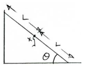
A block of mass $m$ rests on an inclined plane making an angle $\theta$ with the horizontal. The inclined plane (a triangular block of mass $M$ ) is free to slide horizontally without friction. The block of mass $m$ is also free to slide on the larger block of mass $M$ without friction.

(a) Construct the Lagrangian function.

(b) Derive the equations of motion for this system.

(d) Construct the Hamiltonian function.

(e) Find which of the two momenta found in part (c) is a constant of motion and discuss why it is so. If the two blocks start from rest, what is the value of this constant of motion?

Discuss among yourselves the following four conditions that can exist for the Hamiltonian and give several examples of systems exhibiting each of the four conditions.

(a) The Hamiltonian is conserved and equals the total mechanical energy

(b) The Hamiltonian is conserved but does not equal the total mechanical energy

(d) The Hamiltonian is not conserved and does not equal the mechanical total energy.

A block of mass $m$ rests on an inclined plane making an angle $\theta$ with the horizontal. The inclined plane (a triangular block of mass $M$ ) is free to slide horizontally without friction. The block of mass $m$ is also free to slide on the larger block of mass $M$ without friction.

(a) Construct the Lagrangian function.

(b) Derive the equations of motion for this system.

(d) Construct the Hamiltonian function.

(e) Find which of the two momenta found in part (c) is a constant of motion and discuss why it is so. If the two blocks start from rest, what is the value of this constant of motion?

Discuss among yourselves the following four conditions that can exist for the Hamiltonian and give several examples of systems exhibiting each of the four conditions.

a) The Hamiltonian is conserved and equals the total mechanical energy

b) The Hamiltonian is conserved but does not equal the total mechanical energy

c) The Hamiltonian is not conserved but does equal the total mechanical energy

d) The Hamiltonian is not conserved and does not equal the mechanical total energy

Compare the Lagrangian formalism and the Hamiltonian formalism by creating a two-column chart. Label one side “ Lagrangian” and the other side “ Hamiltonian” and discuss the similarities and differences. Here are some ideas to get you started:

What are the basic variables in each formalism?
What are the form and number of the equations of motion derived in each case?
How does the Lagrangian “state space” compare to the Hamiltonian “phase space”?

It can be shown that if $L(q,\dot{q},t)$ is the Lagrangian of a particle moving in one dimension, then $L=L^{\prime }$ where $L^{\prime }(q,\dot{q},t)=L(q,\dot{q},t)+\frac{df}{dt}$ and $f(q,t)$ is an arbitrary function. This problem explores the consequences of this on the Hamiltonian formalism.

(a) Relate the new canonical momentum $p^{\prime }$ , for $L^{\prime }$ , to the old canonical momentum $p$ , for $L$ .

(b) Express the new Hamiltonian $H^{\prime }(q^{\prime },p^{\prime },t)$ for $L^{\prime }$ in terms of the old Hamiltonian $H(q,p,t)$ and $f$ .

(c) Explicitly show that the new Hamilton’s equations for $H^{\prime }$ are equivalent to the old Hamilton’s equations for $H$ .

A massless hoop of radius $R$ is rotating about an axis perpendicular to its central axis at constant angular velocity $\omega$ . A mass $m$ can freely slide around the hoop.

(a) Determine the Lagrangian of the system.

(b) Determine the Hamiltonian of the system. Does it equal the total mechanical energy?

(c) Determine the Lagrangian of the system with respect to a coordinate frame in which $H=T+V_{\text{eff}}$ . What is $V_{\text{ eff}}$ ? What force generates the additional term in $V_{\text{eff}}$ ?

Consider a pendulum of length $L$ attached to the end of rod of length $R$ . The rod is rotating at constant angular velocity $\omega$ in the plane. Assume the pendulum is always taut.

(a) Determine equations of motion.

(b) For what value of $\omega ^{2}R$ is this system the same as a plane pendulum in a constant gravitational field?

A particle of mass $m$ in a gravitational field slides on the inside of a smooth parabola of revolution whose axis is vertical. Using the distance from the axis $r,$ and the azimuthal angle $\varphi$ as generalized coordinates, find the following.

(a) The Lagrangian of the system.

(b) The generalized momenta and the corresponding Hamiltonian

(d) If $\frac{d\varphi }{dt}=0,$ show that the particle can execute small oscillations about the lowest point of the paraboloid and find the frequency of these oscillations.

Consider a particle of mass $m$ which is constrained to move on the surface of a sphere of radius $R$ . There are no external forces of any kind acting on the particle.

(a) What is the number of generalized coordinates necessary to describe the problem?

(b) Choose a set of generalized coordinates and write the Lagrangian of the system.

(d) Prove that the motion of the particle is along a great circle of the sphere.

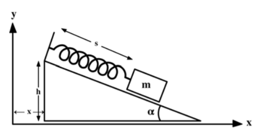
A block of mass $m$ is attached to a wedge of mass $M$ by a spring with spring constant $k$ . The inclined frictionless surface of the wedge makes an angle $\alpha$ to the horizontal. The wedge is free to slide on a horizontal frictionless surface as shown in the figure.

(a) Given that the relaxed length of the spring is $d$ , find the values $s_{0}$ when both book and wedge are stationary.

(b) Find the Lagrangian for the system as a function of the $x$ coordinate of the wedge and the length of spring $s$ . Write down the equations of motion.

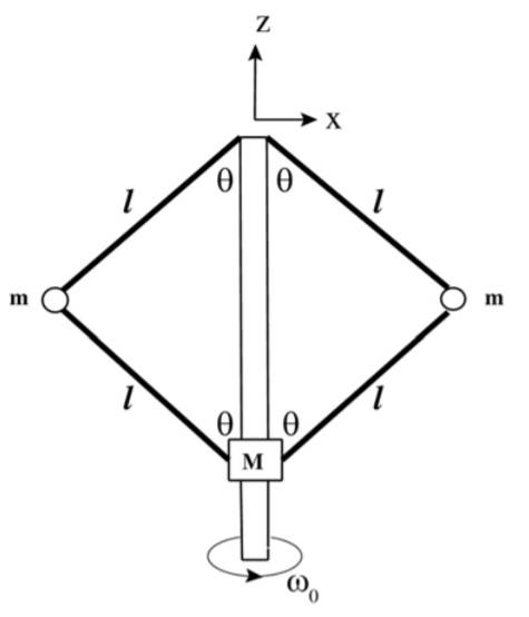
. A fly-ball governor comprises two masses $m$ connected by 4 hinged arms of length $l$ to a vertical shaft and to a mass $M$ which can slide up or down the shaft without friction in a uniform vertical gravitational field as shown in the figure The assembly is constrained to rotate around the axis of the vertical shaft with same angular velocity as that of the vertical shaft. Neglect the mass of the arms, air friction, and assume that the mass $M$ has a negligible moment of inertia. Assume that the whole system is constrained to rotate with a constant angular velocity $\omega _{0}$ .

(a) Choose suitable coordinates and use the Lagrangian to derive equations of motion of the system around the equilibrium position.

(b) Determine the height $z$ of the mass $M$ above its lowest position as a function of $\omega _{0}$ .

(d) Derive a Routhian that provides the Hamiltonian in the rotating system.

(e) Is the total energy of the fly-ball governor in the rotating frame of reference constant in time?

(f) Suppose that the shaft and assembly are not constrained to rotate at a constant angular velocity $\omega _{0}$ , that is, it is allowed to rotate freely at angular velocity $\dot{\varphi}$ . What is the difference in the overall motion?

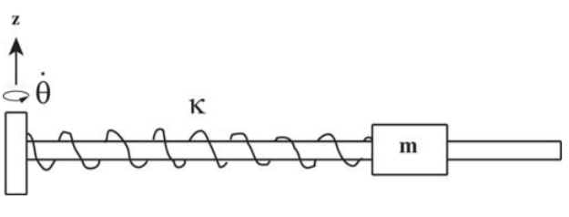
A rigid straight, frictionless, massless, rod rotates about the $z$ axis at an angular velocity $\dot{\theta}$ . A mass $m$ slides along the frictionless rod and is attached to the rod by a massless spring of spring constant $\kappa$ .

(a) Derive the Lagrangian and the Hamiltonian

(b) Derive the equations of motion in the stationary frame using Hamiltonian mechanics.

(d) If the rotation is constrained to have a constant angular velocity $\dot{\theta}=\omega$ then is the non-cyclic Routhian $R_{noncyclic}=H-p_{\theta }\dot{\theta}$ a constant of motion, and does it equal the total energy?

(e) Use the non-cyclic Routhian $R_{noncyclic}$ to derive the radial equation of motion in the rotating frame of reference for the cranked system with $\dot{\theta}=\omega$ .

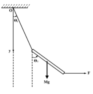
A thin uniform rod of length $2L$ and mass $M$ is suspended from a massless string of length $l$ tied to a nail. Initially the rod hangs vertically. A weak horizontal force $F$ is applied to the rod’s free end.

(a) Write the Lagrangian for this system.

(b) For very short times such that all angles are small, determine the angles that string and the rod make with the vertical. Start from rest at $t=0.$

A uniform ladder of mass $M$ and length $2L$ is leaning against a frictionless vertical wall with its feet on a frictionless horizontal floor. Initially the stationary ladder is released at an angle $\theta _{0}=60^{\circ }$ to the floor. Assume that gravitation field $g=9.81m/s^{2}$ acts vertically downward and that the moment of inertia of the ladder about its midpoint is $I=\frac{1}{3}ML^{2}$ .

(a) Derive the Lagrangian

(b) Derive the Hamiltonian

(d) Use the Lagrangian to derive the equations of motion

(e) Derive the angle $\theta$ at which the ladder loses contact with the vertical wall?

The classical mechanics exam induces Jacob to try his hand at bungee jumping. Assume Jacob’s mass $m$ is suspended in a gravitational field by the bungee of unstretched length $b$ and spring constant $k$ . Besides the longitudinal oscillations due to the bungee jump, Jacob also swings with plane pendulum motion in a vertical plane. Use polar coordinates $r,\phi$ , neglect air drag, and assume that the bungee always is under tension.

(a) Derive the Lagrangian

(b) Determine Lagrange’s equation of motion for angular motion and identify by name the forces contributing to the angular motion.

(c) Determine Lagrange’s equation of motion for radial oscillation and identify by name the forces contributing to the tension in the spring.

(d) Derive the generalized momenta

(e) Determine the Hamiltonian and give all of Hamilton’s equations of motion.

²Recommended****reading: “Classical Mechanics” H. Goldstein, Addison-Wesley, Reading (1950). The present chapter closely follows the notation used by Goldstein to facilitate cross-referencing and reading the many other textbooks that have adopted this notation.

8.S: Hamiltonian Mechanics (Summary)¶

Hamilton’s equations of motion¶

Inserting the generalized momentum into Jacobi’s generalized energy relation was used to define the Hamiltonian function to be

H\left( \mathbf{q},\mathbf{p},t\right) =\mathbf{p\cdot \dot{q}-}L(\mathbf{q}, \mathbf{\dot{q}},t) \tag{8.3}

The Legendre transform of the Lagrange-Euler equations, led to Hamilton’s equations of motion.

\dot{q}_{j} = \frac{\partial H}{\partial p_{j}} \tag{8.25}

\dot{p}_{j} = -\frac{\partial H}{\partial q_{j}}+\left[ \sum_{k=1}^{m} \lambda _{k}\frac{\partial g_{k}}{\partial q_{j}}+Q_{j}^{EXC}\right] \tag{8.26}

The generalized energy equation $(8.8.1)$ gives the time dependence

\frac{dH(\mathbf{q,p,}t\mathbf{)}}{dt}=\sum_{j}\left( \left[ \sum_{k=1}^{m}\lambda _{k}\frac{\partial g_{k}}{\partial q_{j}}+Q_{j}^{EXC} \right] \dot{q}_{j}\right) -\frac{\partial L(\mathbf{q,\dot{q},}t\mathbf{)}}{ \partial t} \tag{8.27}

where

\frac{\partial H}{\partial t}=-\frac{\partial L}{\partial t} \tag{8.24}

The $p_{k},q_{k}$ are treated as independent canonical variables. Lagrange was the first to derive the canonical equations but he did not recognize them as a basic set of equations of motion. Hamilton derived the canonical equations of motion from his fundamental variational principle and made them the basis for a far-reaching theory of dynamics. Hamilton’s equations give $2s$ first-order differential equations for $p_{k},q_{k}$ for each of the $s$ degrees of freedom. Lagrange’s equations give $s$ second-order differential equations for the variables $q_{k},\dot{q}_{k}.$

Routhian reduction technique¶

The Routhian reduction technique is a hybrid of Lagrangian and Hamiltonian mechanics that exploits the advantages of both approaches for solving problems involving cyclic variables. It is especially useful for solving motion in rotating systems in science and engineering. Two Routhians are used frequently for solving the equations of motion of rotating systems. Assuming that the variables between $1\leq i\leq s$ are non-cyclic, while the $m$ variables between $s+1\leq i\leq n$ are ignorable cyclic coordinates, then the two Routhians are:

R_{cyclic}(q_{1},\dots ,q_{n};\dot{q}_{1},\dots ,\dot{q}_{s};p_{s+1},\dots .,p_{n};t) = \sum_{cyclic}^{m}p_{i}\dot{q}_{i}-L=H-\sum_{noncyclic}^{s}p_{i}\dot{q}_{i} \tag{8.65}

R_{noncyclic}(q_{1},\dots ,q_{n};p_{1},\dots ,p_{s};\dot{q}_{s+1},\dots .,\dot{q} _{n};t) = \sum_{noncyclic}^{s}p_{i}\dot{q}_{i}-L=H-\sum_{cyclic}^{m}p_{i} \dot{q}_{i} \tag{8.68}

The Routhian $R_{cyclic}$ is a negative Lagrangian for the non-cyclic variables between $1\leq i\leq s$ , where $s=n-m,$ and is a Hamiltonian for the $m$ cyclic variables between $s+1\leq i\leq n$ . Since the cyclic variables are constants of the Hamiltonian, their solution is trivial, and the number of variables included in the Lagrangian is reduced from $n$ to $s=n-m$ . The Routhian $R_{cyclic}$ is useful for solving some problems in classical mechanics. The Routhian $R_{noncyclic}$ is a Hamiltonian for the non-cyclic variables between $1\leq i\leq s$ , and is a negative Lagrangian for the $m$ cyclic variables between $s+1\leq i\leq n$ . Since the cyclic variables are constants of motion, the Routhian $R_{noncyclic}$ also is a constant of motion but it does not equal the total energy since the coordinate transformation is time dependent. The Routhian $R_{noncyclic}$ is especially valuable for solving rotating many-body systems such as galaxies, molecules, or nuclei, since the Routhian $R_{noncyclic}$ is the Hamiltonian in the rotating body-fixed coordinate frame.

Variable mass systems:¶

Two examples of heavy flexible chains falling in a uniform gravitational field were used to illustrate how variable mass systems can be handled using Lagrangian and Hamiltonian mechanics. The falling-mass system is conservative assuming that both the donor plus the receptor body systems are included.

Comparison of Lagrangian and Hamiltonian mechanics¶

Lagrangian and the Hamiltonian dynamics are two powerful and related variational algebraic formulations of mechanics that are based on Hamilton’s action principle. They can be applied to any conservative degrees of freedom as discussed in chapters 7, 9, and 16. Lagrangian and Hamiltonian mechanics both concentrate solely on active forces and can ignore internal forces. They can handle many-body systems and allow convenient generalized coordinates of choice. This ability is impractical or impossible using Newtonian mechanics. Thus it is natural to compare the relative advantages of these two algebraic formalisms in order to decide which should be used for a specific problem.

For a system with $n$ generalized coordinates, plus $m$ constraint forces that are not required to be known, then the Lagrangian approach, using a minimal set of generalized coordinates, reduces to only $s=n-m$ second-order differential equations and unknowns compared to the Newtonian approach where there are $n+m$ unknowns. Alternatively, use of Lagrange multipliers allows determination of the constraint forces resulting in $n+m$ second order equations and unknowns. The Lagrangian potential function is limited to conservative forces, Lagrange multipliers can be used to handle holonomic forces of constraint, while generalized forces can be used to handle non-conservative and non-holonomic forces. The advantage of the Lagrange equations of motion is that they can deal with any type of force, conservative or non-conservative, and they directly determine $q$ , $\dot{q}$ rather than $q,p$ which then requires relating $p$ to $\dot{q}$ .

For a system with $n$ generalized coordinates, the Hamiltonian approach determines $2n$ first-order differential equations which are easier to solve than second-order equations. However, the $2n$ solutions must be combined to determine the equations of motion. The Hamiltonian approach is superior to the Lagrange approach in its ability to obtain an analytical solution of the integrals of the motion. Hamiltonian dynamics also has a means of determining the unknown variables for which the solution assumes a soluble form. Important applications of Hamiltonian mechanics are to quantum mechanics and statistical mechanics, where quantum analogs of $q_{i}$ and $p_{i},$ can be used to relate to the fundamental variables of Hamiltonian mechanics. This does not apply for the variables $q_{i}$ and $\dot{q}_{i}$ of Lagrangian mechanics. The Hamiltonian approach is especially powerful when the system has $m$ cyclic variables, then the $m$ conjugate momenta $p_{i}$ are constants. Thus the $m$ conjugate variables $\left( q_{i},p_{i}\right)$ can be factored out of the Hamiltonian, which reduces the number of conjugate variables required to $n-m$ . This is not possible using the Lagrangian approach since, even though the $m$ coordinates $q_{i}$ can be factored out, the velocities $\dot{q}_{i}$ still must be included, thus the $n$ conjugate variables must be included. The Lagrange approach is advantageous for obtaining a numerical solution of systems in classical mechanics. However, Hamiltonian mechanics expresses the variables in terms of the fundamental canonical variables $(\mathbf{q,p})$ which provides a more fundamental insight into the underlying physics.²

Footnotes¶

Discussions with Professor Frank Wolfs stimulated inclusion of these two examples of moving chains.
↩