4.1: Introduction to Nonlinear Systems and Chaos
In nature only a subset of systems have equations of motion that are linear. Contrary to the impression given by the analytic solutions presented in undergraduate physics courses, most dynamical systems in nature exhibit non-linear behavior that leads to complicated motion. The solutions of non-linear equations usually do not have analytic solutions, superposition does not apply, and they predict phenomena such as attractors, discontinuous period bifurcation, extreme sensitivity to initial conditions, rolling motion, and chaos. During the past four decades, exciting discoveries have been made in classical mechanics that are associated with the recognition that nonlinear systems can exhibit chaos. Chaotic phenomena have been observed in most fields of science and engineering such as, weather patterns, fluid flow, motion of planets in the solar system, epidemics, changing populations of animals, birds and insects, and the motion of electrons in atoms. The complicated dynamical behavior predicted by non-linear differential equations is not limited to classical mechanics, rather it is a manifestation of the mathematical properties of the solutions of the differential equations involved, and thus is generally applicable to solutions of first or second-order non-linear differential equations. It is important to understand that the systems discussed in this chapter follow a fully deterministic evolution predicted by the laws of classical mechanics, the evolution for which is based on the prior history. This behavior is completely different from a random walk where each step is based on a random process. The complicated motion of deterministic non-linear systems stems in part from sensitivity to the initial conditions. There are many examples of turbulent and laminar flow.
The French mathematician Poincaré is credited with being the first to recognize the existence of chaos during his investigation of the gravitational three-body problem in celestial mechanics. At the end of the nineteenth century Poincaré noticed that such systems exhibit high sensitivity to initial conditions characteristic of chaotic motion, and the existence of nonlinearity which is required to produce chaos. Poincaré’s work received little notice, in part it was overshadowed by the parallel development of the Theory of Relativity and quantum mechanics at the start of the century. In addition, solving nonlinear equations of motion is difficult, which discouraged work on nonlinear mechanics and chaotic motion. The field blossomed during the when computers became sufficiently powerful to solve the nonlinear equations required to calculate the long-time histories necessary to document the evolution of chaotic behavior.
Laplace, and many other scientists, believed in the deterministic view of nature which assumes that if the position and velocities of all particles are known, then one can unambiguously predict the future motion using Newtonian mechanics. Researchers in many fields of science now realize that this “clockwork universe" is invalid. That is, knowing the laws of nature can be insufficient to predict the evolution of nonlinear systems in that the time evolution can be extremely sensitive to the initial conditions even though they follow a completely deterministic development. There are two major classifications of nonlinear systems that lead to chaos in nature. The first classification encompasses nondissipative Hamiltonian systems such as Poincaré’s three-body celestial mechanics system. The other main classification involves driven, damped, non-linear oscillatory systems.
Nonlinearity and chaos is a broad and active field and thus this chapter will focus only on a few examples that illustrate the general features of non-linear systems. Weak non-linearity is used to illustrate bifurcation and asymptotic attractor solutions for which the system evolves independent of the initial conditions. The common sinusoidally-driven linearly-damped plane pendulum illustrates several features characteristic of the evolution of a non-linear system from order to chaos. The impact of non-linearity on wavepacket propagation velocities and the existence of soliton solutions is discussed. The example of the three-body problem is discussed in chapter 11. The transition from laminar flow to turbulent flow is illustrated by fluid mechanics discussed in chapter 16.8. Analytic solutions of nonlinear systems usually are not available and thus one must resort to computer simulations. As a consequence the present discussion focuses on the main features of the solutions for these systems and ignores how the equations of motion are solved.
4.2: Weak Nonlinearity
Most physical oscillators become non-linear with increase in amplitude of the oscillations. Consequences of non-linearity include breakdown of superposition, introduction of additional harmonics, and complicated chaotic motion that has great sensitivity to the initial conditions as illustrated in this chapter. Weak non-linearity is interesting since perturbation theory can be used to solve the non-linear equations of motion.
The potential energy function for a linear oscillator has a pure parabolic shape about the minimum location, that is, where is the location of the minimum. Weak non-linear systems have small amplitude oscillations about the minimum allowing use of the Taylor expansion
By definition, at the minimum and thus Equation 4.1 can be written as
For small amplitude oscillations the system is linear when only the second-order term in Equation 4.2 is significant. The linearity for small amplitude oscillations greatly simplifies description of the oscillatory motion in that superposition applies, and complicated chaotic motion is avoided. For slightly larger amplitude motion, where the higher-order terms in the expansion are still much smaller than the second-order term, then perturbation theory can be used as illustrated by the simple plane pendulum which is non linear since the restoring force equals
This is linear only at very small angles where the higher-order terms in the expansion can be neglected. Consider the equation of motion at small amplitudes for the harmonically-driven, linearly-damped plane pendulum
where only the first two terms in the expansion 4.3 have been included. It was shown in chapter 3 that when then the steady-state solution of Equation 4.4 is of the form
Insert this first-order solution into Equation 4.4, then the cubic term in the expansion gives a term . Thus the perturbation expansion to third order involves a solution of the form
This perturbation solution shows that the non-linear term has distorted the signal by addition of the third harmonic of the driving frequency with an amplitude that depends sensitively on . This illustrates that the superposition principle is not obeyed for this non-linear system, but, if the non-linearity is weak, perturbation theory can be used to derive the solution of a non-linear equation of motion.
Figure 4.2.1 illustrates that for a potential the non-linear term are greatest at the maximum amplitude which makes the total energy contours in state-space more rectangular than the elliptical shape for the harmonic oscillator as shown in figure (3.4.2). The solution is of the form given in Equation 4.6.
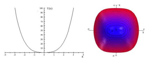
Figure 4.2.1:The left side shows the potential energy for a symmetric potential . The right side shows the contours of constant total energy on a state-space diagram.
4.3: Bifurcation and Point Attractors
Interesting new phenomena, such as bifurcation, and attractors, occur when the non-linearity is large. In chapter 3 it was shown that the state-space diagram for an undamped harmonic oscillator is an ellipse with dimensions defined by the total energy of the system. As shown in figure (3.5.1), for the damped harmonic oscillator, the state-space diagram spirals inwards to the origin due to dissipation of energy. Non-linearity distorts the shape of the ellipse or spiral on the state-space diagram, and thus the state-space, or corresponding phase-space, diagrams, provide useful representations of the motion of linear and non-linear periodic systems.
The complicated motion of non-linear systems makes it necessary to distinguish between transient and asymptotic behavior. The damped harmonic oscillator executes a transient spiral motion that asymptotically approaches the origin. The transient behavior depends on the initial conditions, whereas the asymptotic limit of the steady-state solution is a specific location, that is called a point attractor. The point attractor for damped motion in the anharmonic potential well
is at the minimum, which is the origin of the state-space diagram as shown in figure (4.2.1).
The more complicated one-dimensional potential well
shown in Figure 4.3.1, has two minima that are symmetric about with a saddle of height 8.
The kinetic plus potential energies of a particle with mass released in this potential, will be assumed to be given by
The state-space plot in Figure 4.3.1 shows contours of constant energy with the minima at . At slightly higher total energy the contours are closed loops around either of the two minima at . At total energies above the saddle energy of 8 the contours are peanut-shaped and are symmetric about the origin. Assuming that the motion is weakly damped, then a particle released with total energy which is higher than will follow a peanut-shaped spiral trajectory centered at in the state-space diagram for . For there are two separate solutions for the two minimum centered at and . This is an example of bifurcation where the one solution for bifurcates into either of the two solutions for .
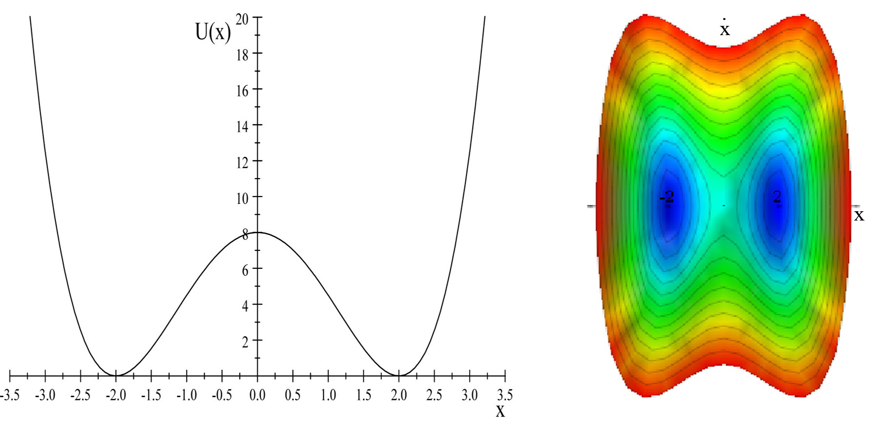
Figure 4.3.1:The left side shows the potential energy for a bimodal symmetric potential . The right-hand figure shows contours of the sum of kinetic and potential energies on a state-space diagram. For total energies above the saddle point the particle follows peanut-shaped trajectories in statespace centered around . For total energies below the saddle point the particle will have closed trajectories about either of the two symmetric minima located at . Thus the system solution bifurcates when the total energy is below the saddle point.
For an initial total energy damping will result in spiral trajectories of the particle that will be trapped in one of the two minima. For the particle trajectories are centered giving the impression that they will terminate at when the kinetic energy is dissipated. However, for the particle will be trapped in one of the two minimum and the trajectory will terminate at the bottom of that potential energy minimum occurring at . These two possible terminal points of the trajectory are called point attractors. This example appears to have a single attractor for which bifurcates leading to two attractors at for . The determination as to which minimum traps a given particle depends on exactly where the particle starts in state space and the damping etc. That is, for this case, where there is symmetry about the -axis, the particle has an initial total energy then the initial conditions with radians of state space will lead to trajectories that are trapped in the left minimum, and the other radians of state space will be trapped in the right minimum. Trajectories starting near the split between these two halves of the starting state space will be sensitive to the exact starting phase. This is an example of sensitivity to initial conditions.
4.4: Limit Cycles
Poincaré-Bendixson theorem
Coupled first-order differential equations in two dimensions of the form
occur frequently in physics. The state-space paths do not cross for such two-dimensional autonomous systems, where an autonomous system is not explicitly dependent on time.
The Poincaré-Bendixson theorem states that, state-space, and phase-space, can have three possible paths:
closed paths, like the elliptical paths for the undamped harmonic oscillator,
terminate at an equilibrium point as , like the point attractor for a damped harmonic oscillator,
tend to a limit cycle as .
The limit cycle is unusual in that the periodic motion tends asymptotically to the limit-cycle attractor independent of whether the initial values are inside or outside the limit cycle. The balance of dissipative forces and driving forces often leads to limit-cycle attractors, especially in biological applications. Identification of limit-cycle attractors, as well as the trajectories of the motion towards these limit-cycle attractors, is more complicated than for point attractors.
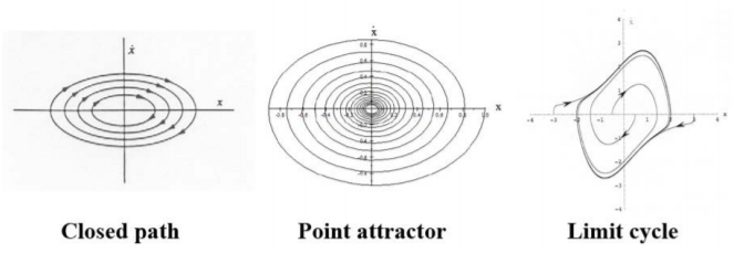
Figure 4.4.1:The Poincaré-Bendixson theorem allows the following three scenarios for two-dimensional autonomous systems. (1) Closed paths as illustrated by the undamped harmonic oscillator. (2) Terminate at an equilibrium point as , as illustrated by the damped harmonic oscillator, and (3) Tend to a limit cycle as as illustrated by the van der Pol oscillator.
van der Pol damped harmonic oscillator
The van der Pol damped harmonic oscillator illustrates a non-linear equation that leads to a well-studied, limit-cycle attractor that has important applications in diverse fields. The van der Pol oscillator has an equation of motion given by
The non-linear damping term is unusual in that the sign changes when leading to positive damping for and negative damping for To simplify Equation 4.11, assume that the term that is, .
This equation was studied extensively during the 1920’s and 1930’s by the Dutch engineer, Balthazar van der Pol, for describing electronic circuits that incorporate feedback. The form of the solution can be simplified by defining a variable Then the second-order Equation 4.11 can be expressed as two coupled first-order equations.
It is advantageous to transform the state space to polar coordinates by setting
and using the fact that . Therefore
Similarly for the angle coordinate
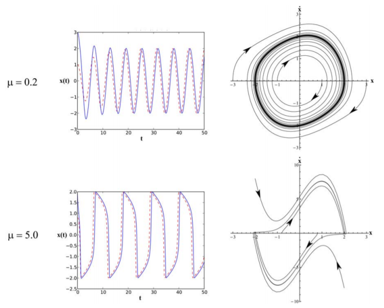
Figure 4.4.2:Solutions of the van der Pol system for top row and bottom row, assuming that . The left column shows the time dependence . The right column shows the corresponding state space plots. Upper: Weak nonlinearity, ; At large times the solution tends to one limit cycle for initial values inside or outside the limit cycle attractor. The amplitude for two initial conditions approaches an approximately harmonic oscillation. Lower: Strong nonlinearity, ; Solutions approach a common limit cycle attractor for initial values inside or outside the limit cycle attractor while the amplitude approaches a common approximate square-wave oscillation.
Multiply Equation 4.16 by and 4.17 by and subtract gives
Equations 4.15 and 4.18 allow the van der Pol equations of motion to be written in polar coordinates
The non-linear terms on the right-hand side of equations 4.19-4.20 have a complicated form.
Weak non-linearity: 
In the limit that , equations 4.19, 4.20 correspond to a circular state-space trajectory similar to the harmonic oscillator. That is, the solution is of the form
where and are arbitrary parameters. For weak non-linearity, the angular Equation 4.20 has a rotational frequency that is unity since the term changes sign twice per period, in addition to the small value of . For and the radial Equation 4.19 has a sign of the term that is positive and thus the radius increases monotonically to unity. For the bracket is predominantly negative resulting in a spiral decrease in the radius. Thus, for very weak non-linearity, this radial behavior results in the amplitude spiralling to a well defined limit-cycle attractor value of as illustrated by the state-space plots in Figure 4.4.2 for cases where the initial condition is inside or external to the circular attractor. The final amplitude for different initial conditions also approach the same asymptotic behavior.
Dominant non-linearity: 
For the case where the non-linearity is dominant, that is , then as shown in Figure 4.4.2, the system approaches a well defined attractor, but in this case it has a significantly skewed shape in state-space, while the amplitude approximates a square wave. The solution remains close to until and then it relaxes quickly to with This is followed by the mirror image. This behavior is called a relaxed vibration in that a tension builds up slowly then dissipates by a sudden relaxation process. The seesaw is an extreme example of a relaxation oscillator where the seesaw angle switches spontaneously from one solution to the other when the difference in their moment arms changes sign.
The study of feedback in electronic circuits was the stimulus for study of this equation by van der Pol. However, Lord Rayleigh first identified such relaxation oscillator behavior in 1880 during studies of vibrations of a stringed instrument excited by a bow, or the squeaking of a brake drum. In his discussion of non-linear effects in acoustics, he derived the equation
Differentiation of Rayleigh’s Equation 4.22 gives
Using the substitution of
leads to the relations
Substituting these relations into Equation 4.23 gives
Multiplying by and rearranging leads to the van der Pol equation
The rhythm of a heartbeat driven by a pacemaker is an important application where the self-stabilization of the attractor is a desirable characteristic to stabilize an irregular heartbeat; the medical term is arrhythmia. The mechanism that leads to synchronization of the many pacemaker cells in the heart and human body due to the influence of an implanted pacemaker is discussed in chapter 14.12. Another biological application of limit cycles is the time variation of animal populations.
In summary the non-linear damping of the van der Pol oscillator leads to a self-stabilized, single limit-cycle attractor that is insensitive to the initial conditions. The van der Pol oscillator has many important applications such as bowed musical instruments, electrical circuits, and human anatomy as mentioned above. The van der Pol oscillator illustrates the complicated manifestations of the motion that can be exhibited by non-linear systems.
4.5: Harmonically-driven, linearly-damped, plane pendulum
The harmonically-driven, linearly-damped, plane pendulum illustrates many of the phenomena exhibited by non-linear systems as they evolve from ordered to chaotic motion. It illustrates the remarkable fact that determinism does not imply either regular behavior or predictability. The well-known, harmonically-driven linearly-damped pendulum provides an ideal basis for an introduction to non-linear dynamics[1].
Consider a harmonically-driven linearly-damped plane pendulum of moment of inertia and mass in a gravitational field that is driven by a torque due to a force acting at a moment arm . The damping term is and the angular displacement of the pendulum, relative to the vertical, is . The equation of motion of the harmonically-driven linearly-damped simple pendulum can be written as
Note that the sinusoidal restoring force for the plane pendulum is non-linear for large angles . The natural period of the free pendulum is
A dimensionless parameter , which is called the drive strength, is defined by
The equation of motion 4.28 can be generalized by introducing dimensionless units for both time and relative drive frequency defined by
In addition, define the inverse damping factor as
These definitions allow Equation 4.28 to be written in the dimensionless form
The behavior of the angle for the driven damped plane pendulum depends on the drive strength and the damping factor . Consider the case where Equation 4.33 is evaluated assuming that the damping coefficient , and that the relative angular frequency which is close to resonance where chaotic phenomena are manifest. The Runge-Kutta method is used to solve this non-linear equation of motion.
Close to Linearity
For drive strength the amplitude is sufficiently small that superposition applies, and the solution is identical to that for the driven linearly-damped linear oscillator. As shown in Figure 4.5.1, once the transient solution dies away, the steady-state solution asymptotically approaches one attractor that has an amplitude of radians and a phase shift with respect to the driving force. The abscissa is given in units of the dimensionless time . The transient solution depends on the initial conditions and dies away after about 5 periods, whereas the steady-state solution is independent of the initial conditions and has a state-space diagram that has an elliptical shape, characteristic of the harmonic oscillator. For all initial conditions, the time dependence and state space diagram for steady-state motion approaches a unique solution, called an “attractor”, that is, the pendulum oscillates sinusoidally with a given amplitude at the frequency of the driving force and with a constant phase shift , i.e.
This solution is identical to that for the harmonically-driven, linearly-damped, linear oscillator discussed in chapter 3.6.
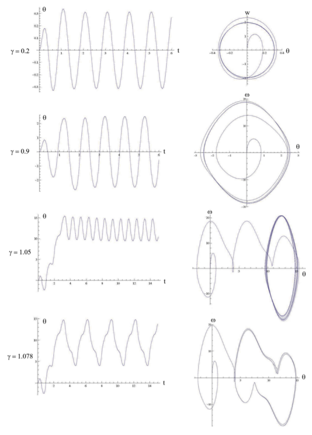
Figure 4.5.1:Motion of the driven damped pendulum for drive strengths of , , , and . The left side shows the time dependence of the deflection angle with the time axis expressed in dimensionless units . The right side shows the corresponding state-space plots. These plots assume , , and the motion starts with .
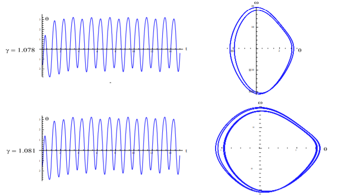
Figure 4.5.2:The driven damped pendulum assuming that , , with initial conditions , . The system exhibits period-two motion for drive strengths of as shown by the state space diagram for cycles . For the system exhibits period-four motion shown for cycles .
Weak nonlinearity
Figure 4.5.1 shows that for drive strength , after the transient solution dies away, the steady-state solution settles down to one attractor that oscillates at the drive frequency with an amplitude of slightly more than radians for which the small angle approximation fails. The distortion due to the non-linearity is exhibited by the non-elliptical shape of the state-space diagram.
The observed behavior can be calculated using the successive approximation method discussed in chapter 4.2. That is, close to small angles the sine function can be approximated by replacing
in Equation 4.33 to give
As a first approximation assume that
then the small term in Equation 4.35 contributes a term proportional to . But
That is, the nonlinearity introduces a small term proportional to . Since the right-hand side of Equation 4.35 is a function of only then the terms in and on the left hand side must contain the third harmonic term. Thus a better approximation to the solution is of the form
where the admixture coefficient . This successive approximation method can be repeated to add additional terms proportional to where is an integer with . Thus the nonlinearity introduces progressively weaker -fold harmonics to the solution. This successive approximation approach is viable only when the admixture coefficient Note that these harmonics are integer multiples of , thus the steady-state response is identical for each full period even though the state space contours deviate from an elliptical shape.
Onset of complication
Figure 4.5.1 shows that for the drive strength is sufficiently strong to cause the transient solution for the pendulum to rotate through two complete cycles before settling down to a single steady-state attractor solution at the drive frequency. However, this attractor solution is shifted two complete rotations relative to the initial condition. The state space diagram clearly shows the rolling motion of the transient solution for the first two periods prior to the system settling down to a single steady-state attractor. The successive approximation approach completely fails at this coupling strength since oscillates through large values that are multiples of
Figure 4.5.1 shows that for drive strength the motion evolves to a much more complicated periodic motion with a period that is three times the period of the driving force. Moreover the amplitude exceeds corresponding to the pendulum oscillating over top dead center with the centroid of the motion offset by from the initial condition. Both the state-space diagram, and the time dependence of the motion, illustrate the complexity of this motion which depends sensitively on the magnitude of the drive strength in addition to the initial conditions, and damping factor as is shown in Figure 4.5.2
Period doubling and bifurcation
For drive strength with the initial condition the system exhibits a regular motion with a period that is three times the drive period. In contrast, if the initial condition is then, as shown in Figure 4.5.2, the steady-state solution has the drive frequency with no offset in , that is, it exhibits period-one oscillation. This appearance of two separate and very different attractors for using different initial conditions, is called bifurcation.
An additional feature of the system response for is that changing the initial conditions to shows that the amplitude of the even and odd periods of oscillation differ slightly in shape and amplitude, that is, the system really has period-two oscillation. This period-two motion, i.e. period doubling, is clearly illustrated by the state space diagram in that, although the motion still is dominated by period-one oscillations, the even and odd cycles are slightly displaced. Thus, for different initial conditions, the system for bifurcates into either of two attractors that have very different waveforms, one of which exhibits period doubling.
The period doubling exhibited for is followed by a second period doubling when as shown in Figure 4.5.2. With increase in drive strength this period doubling keeps increasing in binary multiples to period 8, 16, 32, 64 etc. Numerically it is found that the threshold for period doubling is from two to four occurs at etc. Feigenbaum showed that this cascade increases with increase in drive strength according to the relation that obeys
where , is called a Feigenbaum number. As this cascading sequence goes to a limit where
Rolling motion
It was shown that for the transient solution causes the pendulum to have angle excursions exceeding , that is, the system rolls over top dead center. For drive strengths in the range the steady-state solution for the system undergoes continuous rolling motion as illustrated in Figure 4.5.3. The time dependence for the angle exhibits a periodic oscillatory motion superimposed upon a monotonic rolling motion, whereas the time dependence of the angular frequency is periodic. The state space plots for rolling motion corresponds to a chain of loops with a spacing of between each loop. The state space diagram for rolling motion is more compactly presented if the origin is shifted by per revolution to keep the plot within bounds as illustrated in Figure 4.5.3c.
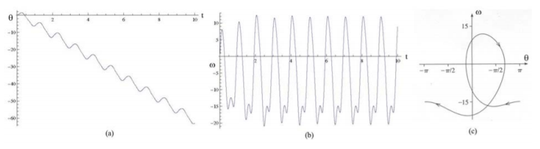
Figure 4.5.3:Rolling motion for the driven damped plane pendulum for . (a) The time dependence of angle increases by per drive period whereas (b) the angular velocity exhibits periodicity. (c) The state space plot for rolling motion is shown with the origin shifted by per revolution to keep the plot within the bounds
Onset of chaos
When the drive strength is increased to then the system does not approach a unique attractor as illustrated by Figure 4.5.4 left which shows state space orbits for cycles . Note that these orbits do not repeat implying the onset of chaos. For drive strengths greater than the driven damped plane pendulum starts to exhibit chaotic behavior. The onset of chaotic motion is illustrated by making a 3-dimensional plot which combines the time coordinate with the state-space coordinates as illustrated in Figure 4.5.4 right. This plot shows 16 trajectories starting at different initial values in the range for . Some solutions are erratic in that, while trying to oscillate at the drive frequency, they never settle down to a steady periodic motion which is characteristic of chaotic motion. Figure 4.5.4 right illustrates the considerable sensitivity of the motion to the initial conditions. That is, this deterministic system can exhibit either order, or chaos, dependent on minuscule differences in initial conditions.
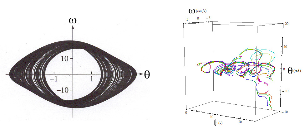
Figure 4.5.4:Left: Space-space orbits for the driven damped pendulum with . Note that the orbits do not repeat for cycles 25 to 200. Right: Time-state-space diagram for . The plot shows 16 trajectories starting with different initial values in the range .
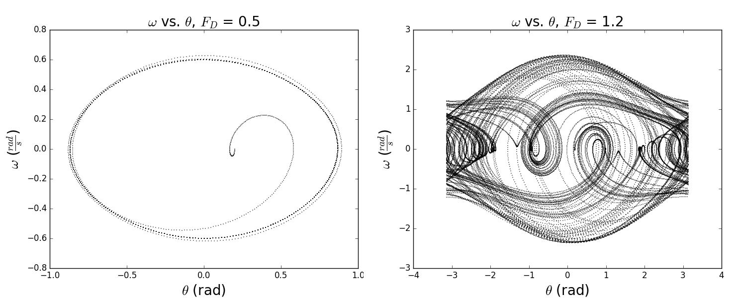
Figure 4.5.5:State-space plots for the harmonically-driven, linearly-damped, pendulum for driving amplitudes of and . These calculations were performed using the Runge-Kutta method by E. Shah, (Private communication)
4.6: Differentiation Between Ordered and Chaotic Motion
Chapter 4.5 showed that motion in non-linear systems can exhibit both order and chaos. The transition between ordered motion and chaotic motion depends sensitively on both the initial conditions and the model parameters. It is surprisingly difficult to unambiguously distinguish between complicated ordered motion and chaotic motion. Moreover, the motion can fluctuate between order and chaos in an erratic manner depending on the initial conditions. The extremely sensitivity to initial conditions of the motion for non-linear systems, makes it essential to have quantitative measures that can characterize the degree of order, and interpret the complicated dynamical motion of systems. As an illustration, consider the harmonically-driven, linearly-damped, pendulum with and driving force where . Figure (4.5.5) shows the state-space plots for two driving amplitudes, which leads to ordered motion, and which leads to possible chaotic motion. It can be seen that for the state-space diagram converges to a single attractor once the transient solution has died away. This is in contrast to the case for where the state-space diagram does not converge to a single attractor, but exhibits possible chaotic motion. Three quantitative measures can be used to differentiate ordered motion from chaotic motion for this system; namely, the Lyapunov exponent, the bifurcation diagram, and the Poincaré section, as illustrated below.
Lyapunov Exponent
The Lyapunov exponent provides a quantitative and useful measure of the instability of trajectories, and how quickly nearby initial conditions diverge. It compares two identical systems that start with an infinitesimally small difference in the initial conditions in order to ascertain whether they converge to the same attractor at long times, corresponding to a stable system, or whether they diverge to very different attractors, characteristic of chaotic motion. If the initial separation between the trajectories in phase space at is , then to first order the time dependence of the difference can be assumed to depend exponentially on time. That is,
where is the Lyapunov exponent. That is, the Lyapunov exponent is defined to be
Systems for which the Lyapunov exponent (negative), converge exponentially to the same attractor solution at long times since for . By contrast, systems for which (positive) diverge to completely different long-time solutions, that is, for . Even for infinitesimally small differences in the initial conditions, systems having a positive Lyapunov exponent diverge to different attractors, whereas when the Lyapunov exponent they correspond to stable solutions.
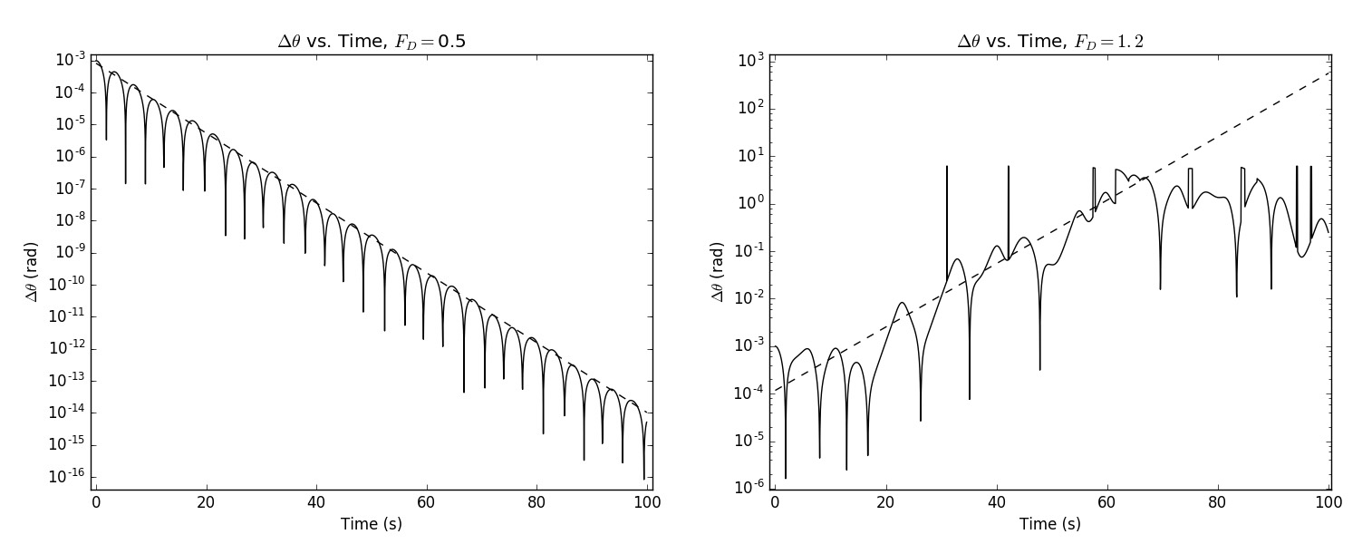
Figure 4.6.1:Lyapunov plots of versus time for two initial starting points differing by . The parameters are , and , and . The Lyapunov exponent for which is drawn as a dashed line, is convergent with . For the exponent is divergent as indicated by the dashed line which as a slope of . These calculations were performed using the Runge-Kutta method by E. Shah, (Private communication)
Figure 4.6.1 illustrates Lyapunov plots for the harmonically-driven, linearly-damped, plane pendulum, with the same conditions discussed in chapter 4.5. Note that for the small driving amplitude the Lyapunov plot converges to ordered motion with an exponent whereas for the plot diverges characteristic of chaotic motion with an exponent The Lyapunov exponent usually fluctuates widely at the local oscillator frequency, and thus the time average of the Lyapunov exponent must be taken over many periods of the oscillation to identify the general trend with time. Some systems near an order-to-chaos transition can exhibit positive Lyapunov exponents for short times, characteristic of chaos, and then converge to negative at longer time implying ordered motion. The Lyapunov exponents are used extensively to monitor the stability of the solutions for non-linear systems. For example the Lyapunov exponent is used to identify whether fluid flow is laminar or turbulent as discussed in chapter 16.8.
A dynamical system in -dimensional phase space will have a set of Lyapunov exponents associated with a set of attractors, the importance of which depend on the initial conditions. Typically one Lyapunov exponent dominates at one specific location in phase space, and thus it is usual to use the maximal Lyapunov exponent to identify chaos. The Lyapunov exponent is a very sensitive measure of the onset of chaos and provides an important test of the chaotic nature for the complicated motion exhibited by non-linear systems.
Bifurcation Diagram
The bifurcation diagram simplifies the presentation of the dynamical motion by sampling the status of the system once per period, synchronized to the driving frequency, for many sets of initial conditions. The results are presented graphically as a function of one parameter of the system in the bifurcation diagram. For example, the wildly different behavior in the driven damped plane pendulum is represented on a bifurcation diagram in Figure 4.6.2, which shows the observed angular velocity of the pendulum sampled once per drive cycle plotted versus drive strength. The bifurcation diagram is obtained by sampling either the angle , or angular velocity , once per drive cycle, that is, it represents the observables of the pendulum using a stroboscopic technique that samples the motion synchronous with the drive frequency. Bifurcation plots also can be created as a function of either the time , the damping factor , the normalized frequency , or the driving amplitude .
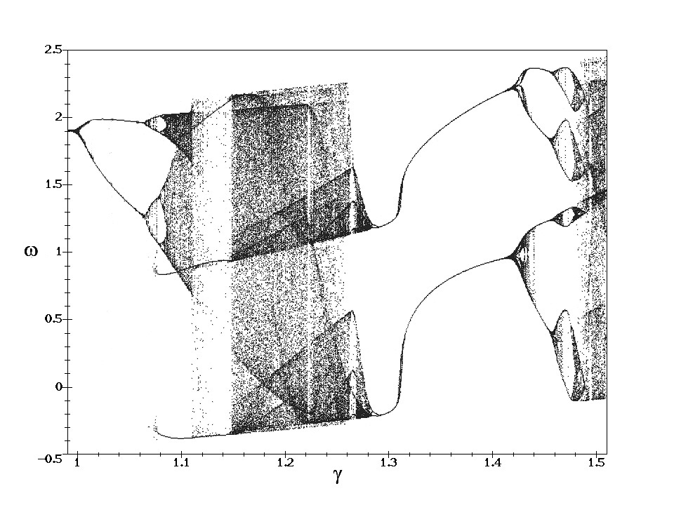
Figure 4.6.2:Bifurcation diagram samples the angular velocity once per period for the driven, linearly-damped, plane pendulum plotted as a function of the drive strength . Regions of period doubling, and chaos, as well as islands of stability all are manifest as the drive strength is changed. Note that the limited number of samples causes broadening of the lines adjacent to bifurcations.
In the domain with drive strength there is one unique angle each drive cycle as illustrated by the bifurcation diagram. For slightly higher drive strength period-two bifurcation behavior results in two different angles per drive cycle. The Lyapunov exponent is negative for this region corresponding to ordered motion. The cascade of period doubling with increase in drive strength is readily apparent until chaos sets in at the critical drive strength when there is a random distribution of sampled angular velocities and the Lyapunov exponent becomes positive. Note that at there is a brief interval of period-6 motion followed by another region of chaos. Around there is a region that is primarily chaotic which is reflected by chaotic values of the angular velocity on the bifurcation plot and large positive values of the Lyapunov exponent. The region around exhibits period three motion and negative Lyapunov exponent corresponding to ordered motion. The region is mainly chaotic and has a large positive Lyapunov exponent. The region with is striking in that this corresponds to rolling motion with reemergence of period one and negative Lyapunov exponent. This period-1 motion is due to a continuous rolling motion of the plane pendulum as shown in figure (4.5.3) where it is seen that the average increases per cycle, whereas the angular velocity exhibits a periodic motion. That is, on average the pendulum is rotating per cycle. Above the system starts to exhibit period doubling followed by chaos reminiscent of the behavior seen at lower values.
These results show that the bifurcation diagram nicely illustrates the order to chaos transitions for the harmonically-driven, linearly-damped, pendulum. Several transitions between order and chaos are seen to occur. The apparent ordered and chaotic regimes are confirmed by the corresponding Lyapunov exponents which alternate between negative and positive values for the ordered and chaotic regions respectively.
Poincaré Section
State-space plots are very useful for characterizing periodic motion, but they become too dense for useful interpretation when the system approaches chaos as illustrated in Figure 4.6.2. Poincaré sections solve this difficulty by taking a stroboscopic sample once per cycle of the state-space diagram. That is, the point on the state space orbit is sampled once per drive frequency. For period-1 motion this corresponds to a single point . For period-2 motion this corresponds to two points etc. For chaotic systems the sequence of state-space sample points follow complicated trajectories. Figure 4.6.3 shows the Poincaré sections for the corresponding state space diagram shown in figure (4.5.5) for cycles 10 to 6000. Note the complicated curves do not cross or repeat. Enlargements of any part of this plot will show increasingly dense parallel trajectories, called fractals, that indicates the complexity of the chaotic cyclic motion. That is, zooming in on a small section of this Poincaré plot shows many closely parallel trajectories. The fractal attractors are surprisingly robust to large differences in initial conditions. Poincaré sections are a sensitive probe of periodic motion for systems where periodic motion is not readily apparent.
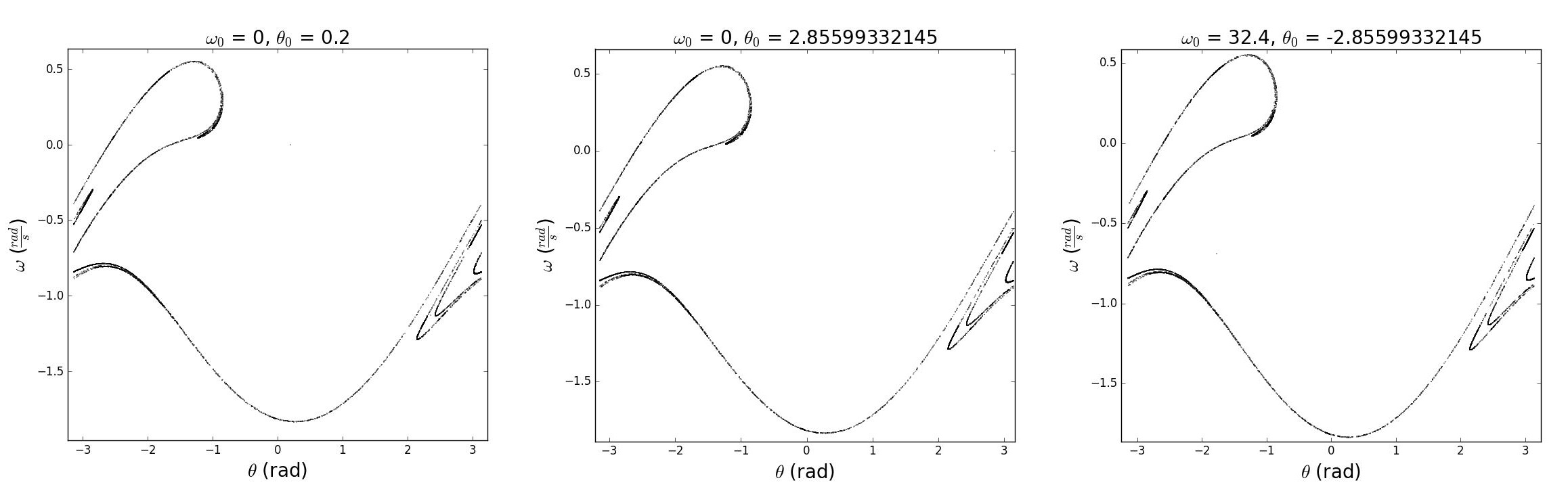
Figure 4.6.3:Three Poincaré section plots for the harmonically-driven, linearly-damped, pendulum for various initial conditions with , , and . These calculations used the Runge-Kutta method and were performed for 6000 cycles by E. Shah (Private communication).
In summary, the behavior of the well-known, harmonically-driven, linearly-damped, plane pendulum becomes remarkably complicated at large driving amplitudes where non-linear effects dominate. That is, when the restoring force is non-linear. The system exhibits bifurcation where it can evolve to multiple attractors that depend sensitively on the initial conditions. The system exhibits both oscillatory, and rolling, solutions depending on the amplitude of the motion. The system exhibits domains of simple ordered motion separated by domains of very complicated ordered motion as well as chaotic regions. The transitions between these dramatically different modes of motion are extremely sensitive to the amplitude and phase of the driver. Eventually the motion becomes completely chaotic. The Lyapunov exponent, bifurcation diagram, and Poincaré section plots, are sensitive measures of the order of the motion. These three sensitive measures of order and chaos are used extensively in many fields in classical mechanics. Considerable computing capabilities are required to elucidate the complicated motion involved in non-linear systems. Examples include laminar and turbulent flow in fluid dynamics and weather forecasting of hurricanes, where the motion can span a wide dynamic range in dimensions from 10-5 to 104 .
4.7: Wave Propagation for Non-linear Systems
Phase, group, and signal velocities
Chapter 3 discussed the wave equation and solutions for linear systems. It was shown that, for linear systems, the wave motion obeys superposition and exhibits dispersion, that is, a frequency-dependent phase velocity, and, in some cases, attenuation. Nonlinear systems introduce intriguing new wave phenomena. For example for nonlinear systems, second, and higher terms must be included in the Taylor expansion given in equation . These second and higher order terms result in the group velocity being a function of that is, group velocity dispersion occurs which leads to the shape of the envelope of the wave packet being time dependent. As a consequence the group velocity in the wave packet is not well defined, and does not equal the signal velocity of the wave packet or the phase velocity of the wavelets. Nonlinear optical systems have been studied experimentally where , which is called slow light, while other systems have which is called superluminal light. The ability to control the velocity of light in such optical systems is of considerable current interest since it has signal transmission applications.
The dispersion relation for a nonlinear system can be expressed as a Taylor expansion of the form
where is used as the independent variable since it is invariant to phase transitions of the system. Note that the factor for the first derivative term is the reciprocal of the group velocity
while the factor for the second derivative term is
which gives the velocity dispersion for the system.
Since
then
The inverse velocities for electromagnetic waves are best represented in terms of the corresponding refractive indices where
and the group refractive index
Then Equation \text{(4.45)} can be written in the more convenient form
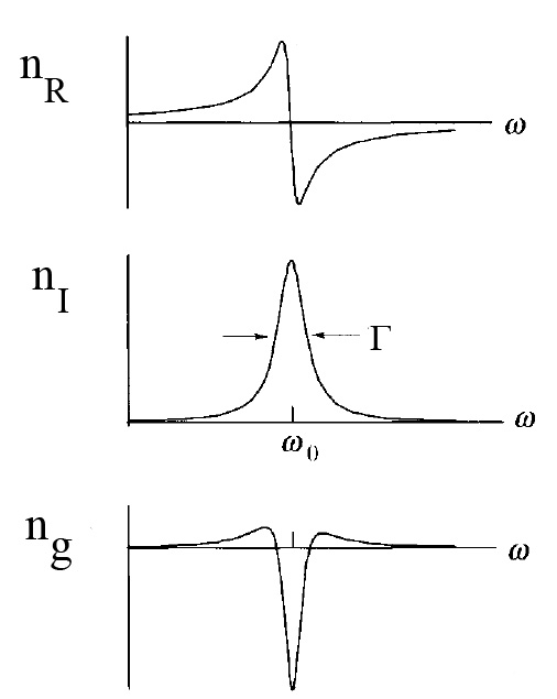
Figure 4.7.1:The real and imaginary parts of the phase refractive index n plus the real part of the group refractive index associated with an isolated atomic resonance.
Wave propagation for an optical system that is subject to a single resonance gives one example of nonlinear frequency response that has applications to optics.
Figure 4.7.1 shows that the real and imaginary parts of the phase refractive index exhibit the characteristic resonance frequency dependence of the sinusoidally-driven, linear oscillator that was discussed in chapter 3.6 and as illustrated in figure (3.6.4). Figure 4.7.1 also shows the group refractive index computed using Equation \text{(4.48)}.
Note that at resonance, is reduced below the non-resonant value which corresponds to superluminal (fast) light, whereas in the wings of the resonance is larger than the non-resonant value corresponding to slow light. Thus the nonlinear dependence of the refractive index on angular frequency leads to fast or slow group velocities for isolated wave packets. Velocities of light as slow as 17 have been observed. Experimentally the energy absorption that occurs on resonance makes it difficult to observe the superluminal electromagnetic wave at resonance.
Note that Sommerfeld and Brillouin showed that even though the group velocity may exceed , the signal velocity, which marks the arrival of the leading edge of the optical pulse, does not exceed , the velocity of light in vacuum, as was postulated by Einstein.
Soliton wave propagation
The soliton is a fascinating and very special wave propagation phenomenon that occurs for certain non-linear systems. The soliton is a self-reinforcing solitary localized wave packet that maintains its shape while traveling long distances at a constant speed. Solitons are caused by a cancellation of phase modulation resulting from non-linear velocity dependence, and the group velocity dispersive effects in a medium. Solitons arise as solutions of a widespread class of weakly-nonlinear dispersive partial differential equations describing many physical systems. Figure 4.7.2 shows a soliton comprising a solitary water wave approaching the coast of Hawaii. While the soliton in Fig. 4.7.2 may appear like a normal wave, it is unique in that there are no other waves accompanying it. This wave was probably created far away from the shore when a normal wave was modulated by a geometrical change in the ocean depth, such as the rising sea floor, which forced it into the appropriate shape for a soliton. The wave then was able to travel to the coast intact, despite the apparently placid nature of the ocean near the beach. Solitons are notable in that they interact with each other in ways very different from normal waves. Normal waves are known for their complicated interference patterns that depend on the frequency and wavelength of the waves. Solitons, can pass right through each other without being a affected at all. This makes solitons very appealing to scientists because soliton waves are more sturdy than normal waves, and can therefore be used to transmit information in ways that are distinctly different than for normal wave motion. For example, optical solitons are used in optical fibers made of a dispersive, nonlinear optical medium, to transmit optical pulses with an invariant shape.

Figure 4.7.2:A solitary wave approaches the coast of Hawaii. (Image: Robert Odom/University of Washington)
Solitons were first observed in 1834 by John Scott Russell (). Russell was an engineer conducting experiments to increase the efficiency of canal boats. His experimental and theoretical investigations allowed him to recreate the phenomenon in wave tanks. Through his extensive studies, Scott Russell noticed that soliton propagation exhibited the following properties:
The waves are stable and hold their shape for long periods of time.
The waves can travel over long distances at uniform speed.
The speed of propagation of the wave depends on the size of the wave, with larger waves traveling faster than smaller waves.
The waves maintained their shape when they collided - seemingly passing right through each other.
Scott Russell’s work was met with skepticism by the scientific community. The problem with the Wave of Translation was that it was an effect that depended on nonlinear effects, whereas previously existing theories of hydrodynamics (such as those of Newton and Bernoulli) only dealt with linear systems. George Biddell Airy, and George Gabriel Stokes, published papers attacking Scott Russell’s observations because the observations could not be explained by their theories of wave propagation in water. Regardless, Scott Russell was convinced of the prime importance of the Wave of Translation, and history proved that he was correct. Scott Russell went on to develop the “wave line” system of hull construction that revolutionized nineteenth century naval architecture, along with a number of other great accomplishments leading him to fame and prominence. Despite all of the success in his career, he continued throughout his life to pursue his studies of the Wave of Translation.
In 1895 Korteweg and de Vries developed a wave equation for surface waves for shallow water.
A solution of this equation has the characteristics of a solitary wave with fixed shape. It is given by substituting the form into the Korteweg-de Vries equation which gives
Integrating with respect to gives
where is a constant of integration. This non-linear equation has a solution
where is a constant. Equation \text{(4.52)} is the equation of a solitary wave moving in the direction at a velocity .
Soliton behavior is observed in phenomena such as tsunamis, tidal bores that occur for some rivers, signals in optical fibers, plasmas, atmospheric waves, vortex filaments, superconductivity, and gravitational fields having cylindrical symmetry. Much work has been done on solitons for fiber optics applications. The soliton’s inherent stability make long-distance transmission possible without the use of repeaters, and could potentially double the transmission capacity.
Before the discovery of solitons, mathematicians were under the impression that nonlinear partial differential equations could not be solved exactly. However, solitons led to the recognition that there are non-linear systems that can be solved analytically. This discovery has prompted much investigation into these so-called “integrable systems.” Such systems are rare, as most non-linear differential equations admit chaotic behavior with no explicit solutions. Integrable systems nevertheless lead to very interesting mathematics ranging from differential geometry and complex analysis to quantum field theory and fluid dynamics.
Many of the fundamental equations in physics (Maxwell’s, Schrödinger’s) are linear equations. However, physicists have begun to recognize many areas of physics in which nonlinearity can result in qualitatively new phenomenon which cannot be constructed via perturbation theory starting from linearized equations. These include phenomena in magnetohydrodynamics, meteorology, oceanography, condensed matter physics, nonlinear optics, and elementary particle physics. For example, the European space mission Cluster detected a soliton-like electrical disturbances that traveled through the ionized gas surrounding the Earth starting about 50,000 kilometers from Earth and traveling towards the planet at about 8 km/s. It is thought that this soliton was generated by turbulence in the magnetosphere.
Efforts to understand the nonlinearity of solitons has led to much research in many areas of physics. In the context of solitons, their particle-like behavior (in that they are localized and preserved under collisions) leads to a number of experimental and theoretical applications. The technique known as bosonization allows viewing particles, such as electrons and positrons, as solitons in appropriate field equations. There are numerous macroscopic phenomena, such as internal waves on the ocean, spontaneous transparency, and the behavior of light in fiber optic cable, that are now understood in terms of solitons. These phenomena are being applied to modern technology.
4.E: Nonlinear Systems and Chaos (Exercises)
Consider the chaotic motion of the driven damped pendulum whose equation of motion is given by
for which the Lyapunov exponent is with time measured in units of the drive period.
Assume that you need to predict with accuracy of , and that the initial value is known to within 10-6 . What is the maximum time horizon for which you can predict to within the required accuracy?
Suppose that you manage to improve the accuracy of the initial value to 10-9 (that is, a thousand-fold improvement). What is the time horizon now for achieving the accuracy of 10-2 ?
By what factor has improved with the improvement in initial measurement.
What does this imply regarding long-term predictions of chaotic motion?
A non-linear oscillator satisfies the equation Find the polar equations for the motion in the state-space diagram. Show that any trajectory that starts within the circle encircle the origin infinitely many times in the clockwise direction. Show further that these trajectories in state space terminate at the origin.
Consider the system of a mass suspended between two identical springs as shown.
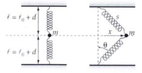
If each spring is stretched a distance to attach the mass at the equilibrium position the mass is subject to two equal and oppositely directed forces of magnitude . Ignore gravity. Show that the potential in which the mass moves is approximately
Construct a state-space diagram for this potential.
A non-linear oscillator satisfies the equation
Find the polar equations for the motion in the state-space diagram. Show that any trajectory that starts in the domain spirals clockwise and tends to the limit cycle . [The same is true of trajectories that start in the domain . ] What is the period of the limit cycle?
A mass moves in one direction and is subject to a constant force when and to a constant force when . Describe the motion by constructing a state space diagram. Calculate the period of the motion in terms of and the amplitude . Disregard damping.
Investigate the motion of an undamped mass subject to a force of the form
4.S: Nonlinear Systems and Chaos (Summary)
The study of the dynamics of non-linear systems remains a vibrant and rapidly evolving field in classical mechanics as well as many other branches of science. This chapter has discussed examples of non-linear systems in classical mechanics. It was shown that the superposition principle is broken even for weak nonlinearity. It was shown that increased nonlinearity leads to bifurcation, point attractors, limit-cycle attractors, and sensitivity to initial conditions.
Limit-cycle attractors
The Poincaré-Bendixson theorem for limit cycle attractors states that the paths, both in state-space and phase-space, can have three possible paths:
closed paths, like the elliptical paths for the undamped harmonic oscillator,
terminate at an equilibrium point as , like the point attractor for a damped harmonic oscillator,
tend to a limit cycle as .
The limit cycle is unusual in that the periodic motion tends asymptotically to the limit-cycle attractor independent of whether the initial values are inside or outside the limit cycle. The balance of dissipative forces and driving forces often leads to limit-cycle attractors, especially in biological applications. Identification of limit-cycle attractors, as well as the trajectories of the motion towards these limit-cycle attractors, is more complicated than for point attractors.
The van der Pol oscillator is a common example of a limit-cycle system that has an equation of motion of the form
The van der Pol oscillator has a limit-cycle attractor that includes non-linear damping and exhibits periodic solutions that asymptotically approach one attractor solution independent of the initial conditions. There are many examples in nature that exhibit similar behavior.
Harmonically-driven, linearly-damped, plane pendulum
The non-linearity of the well-known driven linearly-damped plane pendulum was used as an example of the behavior of non-linear systems in nature. It was shown that non-linearity leads to discontinuous period bifurcation, extreme sensitivity to initial conditions, rolling motion and chaos.
Differentiation between ordered and chaotic motion
Lyapunov exponents, bifurcation diagrams, and Poincaré sections were used to identify the transition from order to chaos. Chapter 16.8 discusses the non-linear Navier-Stokes equations of viscous-fluid flow which leads to complicated transitions between laminar and turbulent flow. Fluid flow exhibits remarkable complexity that nicely illustrates the dominant role that non-linearity can have on the solutions of practical non-linear systems in classical mechanics.
Wave propagation for non-linear systems
Non-linear equations can lead to unexpected behavior for wave packet propagation such as fast or slow light as well as soliton solutions. Moreover, it is notable that some non-linear systems can lead to analytic solutions.
The complicated phenomena exhibited by the above non-linear systems is not restricted to classical mechanics, rather it is a manifestation of the mathematical behavior of the solutions of the differential equations involved. That is, this behavior is a general manifestation of the behavior of solutions for second-order differential equations. Exploration of this complex motion has only become feasible with the advent of powerful computer facilities during the past three decades. The breadth of phenomena exhibited by these examples is manifest in other nonlinear systems, ranging from many-body motion, weather patterns, growth of biological species, epidemics, motion of electrons in atoms, etc. Other examples of non-linear equations of motion not discussed here, are the three-body problem, which is mentioned in chapter 11, and turbulence in fluid flow which is discussed in chapter 16.
It is stressed that the behavior discussed in this chapter is very different from the random walk problem which is a stochastic process where each step is purely random and not deterministic. This chapter has assumed that the motion is fully deterministic and rigorously follows the laws of classical mechanics. Even though the motion is fully deterministic, and follows the laws of classical mechanics, the motion is extremely sensitive to the initial conditions and the non-linearities can lead to chaos. Computer modeling is the only viable approach for predicting the behavior of such non-linear systems. The complexity of solving non-linear equations is the reason that this book will continue to consider only linear systems. Fortunately, in nature, non-linear systems can be approximately linear when the small-amplitude assumption is applicable.
A similar approach is used by the book “Chaotic Dynamics” by Baker and Gollub[Bak96].