11.1: Introduction to Conservative two-body Central Forces
Conservative two-body central forces are important in physics because of the pivotal role that the Coulomb and the gravitational forces play in nature. The Coulomb force plays a role in electrodynamics, molecular, atomic, and nuclear physics, while the gravitational force plays an analogous role in celestial mechanics. Therefore this chapter focuses on the physics of systems involving conservative two-body central forces because of the importance and ubiquity of these conservative two-body central forces in nature.
A conservative two-body central force has the following three important attributes.
Conservative: A conservative force depends only on the particle position, that is, the force is not time dependent. Moreover the work done by the force moving a body between any two points 1 and 2 is path independent. Conservative fields are discussed in chapter 2.10.
Two-body: A two-body force between two bodies depends only on the relative locations of the two interacting bodies and is not influenced by the proximity of additional bodies. For two-body forces acting between bodies, the force on body 1 is the vector superposition of the two-body forces due to the interactions with each of the other bodies. This differs from three-body forces where the force between any two bodies is influenced by the proximity of a third body.
**Central:**A central force field depends on the distance from the origin of the force at point to the body location at point 2, and the force is directed along the line joining them, that is, .
A conservative, two-body, central force combines the above three attributes and can be expressed as,
The force field has a magnitude that depends only on the magnitude of the relative separation vector between the origin of the force at point 1 and point 2 where the force acts, and the force is directed along the line joining them, that is, .
Chapter 2.10 showed that if a two-body central force is conservative, then it can be written as the gradient of a scalar potential energy which is a function of the distance from the center of the force field.
As discussed in chapter 2, the ability to represent the conservative central force by a scalar function greatly simplifies the treatment of central forces.
The Coulomb and gravitational forces both are true conservative, two-body, central forces whereas the nuclear force between nucleons in the nucleus has three-body components. Two bodies interacting via a two-body central force is the simplest possible system to consider, but Equation 11.1 is applicable equally for bodies interacting via two-body central forces because the superposition principle applies for two-body central forces. This chapter will focus first on the motion of two bodies interacting via conservative two-body central forces followed by a brief discussion of the motion for interacting bodies.
11.2: Equivalent one-body Representation for two-body motion
The motion of two bodies, 1 and 2, interacting via two-body central forces, requires 6 spatial coordinates, that is, three each for and . Since the two-body central force only depends on the relative separation of the two bodies, it is more convenient to separate the 6 degrees of freedom into 3 spatial coordinates of relative motion plus 3 spatial coordinates for the center-of-mass location as described in chapter 2.7. It will be shown here that the equation of motion for relative motion of the two-bodies in the center of mass can be represented by an equivalent one-body problem which simplifies the mathematics.
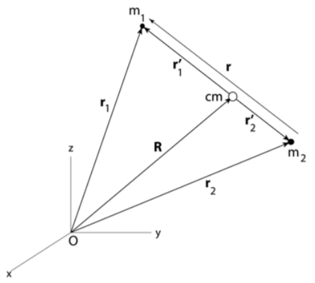
Figure 11.2.1:Center of mass coordinates for the two-body system.
Consider two bodies acted upon by a conservative two-body central force, where the position vectors and specify the location of each particle as illustrated in Figure 11.2.1. An alternate set of six variables would be the three components of the center of mass position vector and the three components specifying the difference vector defined by Figure 11.2.1. Define the vectors and as the position vectors of the masses and with respect to the center of mass. Then
By the definition of the center of mass
and
so that
Therefore
that is,
Similarly;
Substituting these into Equation 11.3 gives
That is, the two vectors are written in terms of the position vector for the center of mass and the position vector for relative motion in the center of mass frame.
Assuming that the two-body central force is conservative and represented by , then the Lagrangian of the two-body system can be written as
Differentiating equations 11.10, with respect to time, and inserting them into the Lagrangian, gives
where the total mass is defined as
and the reduced mass is defined by
or equivalently
The total Lagrangian can be separated into two independent parts
where
Assuming that no external forces are acting, then and the three Lagrange equations for each of the three coordinates of the coordinate can be written as
That is, for a pure central force, the center-of-mass momentum is a constant of motion where
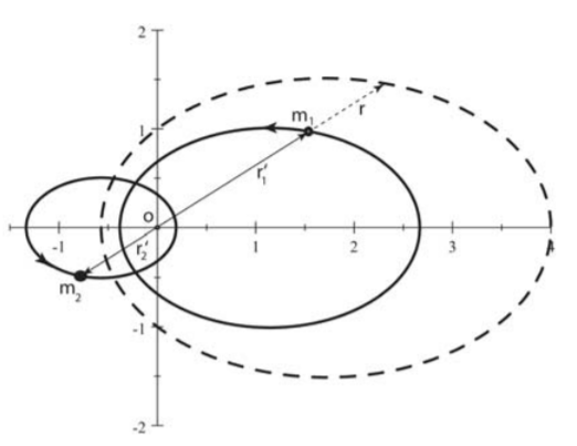
Figure 11.2.2:Orbits of a two-body system with mass ratio of 2 rotating about the center-of-mass, O. The dashed ellipse is the equivalent one-body orbit with the center of force at the focus O.
It is convenient to work in the center-of-mass frame using the effective Lagrangian . In the center-of-mass frame of reference, the translational kinetic energy associated with center-of-mass motion is ignored, and only the energy in the center-of-mass is considered. This center-of-mass energy is the energy involved in the interaction between the colliding bodies. Thus, in the center-of-mass, the problem has been reduced to an equivalent one-body problem of a mass moving about a fixed force center with a path given by which is the separation vector between the two bodies, as shown in figure 11.2.2. In reality, both masses revolve around their center of mass, also called the barycenter, in the center-of-mass frame as shown in Figure 11.2.2. Knowing allows the trajectory of each mass about the center of mass and to be calculated. Of course the true path in the laboratory frame of reference must take into account both the translational motion of the center of mass, in addition to the motion of the equivalent one-body representation relative to the barycenter. Be careful to remember the difference between the actual trajectories of each body, and the effective trajectory assumed when using the reduced mass which only determines the relative separation of the two bodies. This reduction to an equivalent one-body problem greatly simplifies the solution of the motion, but it misrepresents the actual trajectories and the spatial locations of each mass in space. The equivalent one-body representation will be used extensively throughout this chapter.
11.3: Angular Momentum
Angular momentum 
The notation used for the angular momentum vector is where the magnitude is designated by . Be careful not to confuse the angular momentum vector with the Lagrangian Note that the angular momentum for two-body rotation about the center of mass with angular velocity is identical when evaluated in either the laboratory or equivalent two-body representation. That is, using equations and
The center-of-mass Lagrangian leads to the following two general properties regarding the angular momentum vector .
The motion lies entirely in a plane perpendicular to the fixed direction of the total angular momentum vector. This is because
that is, the radius vector is in the plane perpendicular to the total angular momentum vector. Thus, it is possible to express the Lagrangian in polar coordinates, rather than spherical coordinates. In polar coordinates the center-of-mass Lagrangian becomes
If the potential is spherically symmetric, then the polar angle is cyclic and therefore Noether’s theorem gives that**the angular momentum is a constant of motion. That is, since then the Lagrange equations imply that
where the vectors and imply that Equation \text{(11.23)} refers to three independent equations corresponding to the three components of these vectors. Thus the angular momentum conjugate to is a constant of motion. The generalized momentum is a first integral of the motion which equals
where the magnitude of the angular momentum , and the direction both are constants of motion.
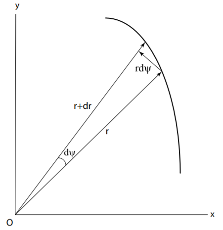
Figure 11.3.1:Area swept out by the radius vector in the time dt.
A simple geometric interpretation of Equation \text{(11.24)} is illustrated in Figure 11.3.1. The radius vector sweeps out an area in time where
and the vector is perpendicular to the plane. The rate of change of area is
But the angular momentum is
Thus the conservation of angular momentum implies that the areal velocity also is a constant of motion. This fact is called Kepler’s second law of planetary motion which he deduced in 1609 based on Tycho Brahe’s 55 years of observational records of the motion of Mars. Kepler’s second law implies that a planet moves fastest when closest to the sun and slowest when farthest from the sun. Note that Kepler’s second law is a statement of the conservation of angular momentum which is independent of the radial form of the central potential.
11.4: Equations of Motion
The equations of motion for two bodies interacting via a conservative two-body central force can be determined using the center of mass Lagrangian, given by equation . For the radial coordinate, the operator equation for Lagrangian mechanics leads to
But
therefore the radial equation of motion is
Similarly, for the angular coordinate, the operator equation leads to equation . That is, the angular equation of motion for the magnitude of is
Lagrange’s equations have given two equations of motion, one dependent on radius and the other on the polar angle . Note that the radial acceleration is just a statement of Newton’s Laws of motion for the radial force in the center-of-mass system of
This can be written in terms of an effective potential
which leads to an equation of motion
Since , the second term in Equation \text{(11.33)} is the usual centrifugal force that originates because the variable is in a non-inertial, rotating frame of reference. Note that the angular equation of motion is independent of the radial dependence of the conservative two-body central force.
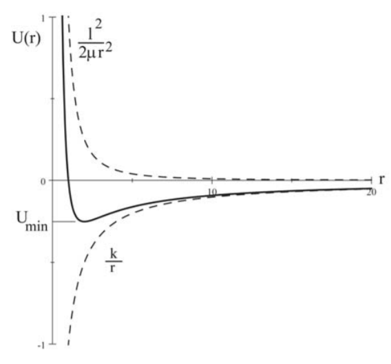
Figure 11.4.1:The attractive inverse-square law potential , the centrifugal potential , and the combined effective bound potential.
Figure 11.4.1 shows, by dashed lines, the radial dependence of the potential corresponding to the attractive inverse square law force, that is , and the potential corresponding to the centrifugal term corresponding to a repulsive centrifugal force. The sum of these two potentials , shown by the solid line, has a minimum value at a certain radius similar to that manifest by the diatomic molecule discussed in example .
It is remarkable that the six-dimensional equations of motion, for two bodies interacting via a two-body central force, has been reduced to trivial center-of-mass translational motion, plus a one-dimensional one-body problem given by \text{(11.34)} in terms of the relative separation and an effective potential .
11.5: Differential Orbit Equation
The differential orbit equation relates the shape of the orbital motion, in plane polar coordinates, to the radial dependence of the two-body central force. A Binet coordinate transformation, which depends on the functional form of can simplify the differential orbit equation. For the inverse-square law force, the best Binet transformed variable is which is defined to be
Inserting the transformed variable into equation gives
From the definition of the new variable
Differentiating again gives
Substituting these into Lagrange’s radial equation of motion gives
Binet’s differential orbit equation directly relates and which determines the overall shape of the orbit trajectory. This shape is crucial for understanding the orbital motion of two bodies interacting via a two-body central force. Note that for the special case of an inverse square-law force, that is where , then the right-hand side of Equation \text{(11.39)} equals a constant since the orbital angular momentum is a conserved quantity.
11.6: Hamiltonian
Since the center-of-mass Lagrangian is not an explicit function of time, then
Thus the center-of mass Hamiltonian is a constant of motion. However, since the transformation to center of mass can be time dependent, then that is, it does not include the total energy because the kinetic energy of the center-of-mass motion has been omitted from . Also, since no transformation is involved, then
That is, the center-of-mass Hamiltonian equals the center-of-mass total energy. The center-of-mass Hamiltonian then can be written using the effective potential in the form
It is convenient to express the center-of-mass Hamiltonian in terms of the energy equation for the orbit in a central field using the transformed variable . Substituting equations and into the Hamiltonian Equation \text{(11.42)} gives theenergy equation of the orbit
Energy conservation allows the Hamiltonian to be used to solve problems directly. That is, since
then
The time dependence can be obtained by integration
An inversion of this gives the solution in the standard form However, it is more interesting to find the relation between and From relation \text{(11.46)} for then
while equation gives
Therefore
which can be used to calculate the angular coordinate. This gives the relation between the radial and angular coordinates which specifies the trajectory.
Although equations \text{(11.45)} and \text{(11.49)} formally give the solution, the actual solution can be derived analytically only for certain specific forms of the force law and these solutions differ for attractive versus repulsive interactions.
11.7: General Features of the Orbit Solutions
It is useful to look at the general features of the solutions of the equations of motion given by the equivalent one-body representation of the two-body motion. These orbits depend on the net center of mass energy There are five possible situations depending on the center-of-mass total energy .
The trajectory is hyperbolic and has a minimum distance, but no maximum. The distance of closest approach is given when At the turning point
It can be shown that the orbit for this case is parabolic.
For this case the equivalent orbit has both a maximum and minimum radial distance at which At the turning points the radial kinetic energy term is zero so For the attractive inverse square law force the path is an ellipse with the focus at the center of attraction (Figure ), which is Kepler’s First Law. During the time that the radius ranges from to and back the radius vector turns through an angle which is given by
The general path prescribes a rosette shape which is a closed curve only if is a rational fraction of .
In this case is a constant implying that the path is circular since
For this case the square root is imaginary and there is no real solution.
In general the orbit is not closed, and such open orbits do not repeat. Bertrand’s Theorem states that the inverse-square central force, and the linear harmonic oscillator, are the only radial dependences of the central force that lead to stable closed orbits.
11.8: Inverse-square, two-body, central force
The most important conservative, two-body, central interaction is the attractive inverse-square law force, which is encountered in both gravitational attraction and the Coulomb force. This force can be written in the form
The force constant is defined to be negative for an attractive force and positive for a repulsive force. In S.I. units the force constant for the gravitational force and for the Coulomb force. Note that this sign convention is the opposite of what is used in many books which use a negative sign in Equation \text{(11.52)} and assume to be positive for an attractive force and negative for a repulsive force.
The conservative, inverse-square, two-body, central force is unique in that the underlying symmetries lead to four conservation laws, all of which are of pivotal importance in nature.
Conservation of angular momentum: Like all conservative central forces, the inverse-square central two-body force conserves angular momentum as proven in chapter 11.3.
Conservation of energy: This conservative central force can be represented in terms of a scalar potential energy as given by equation , where for this central force
Moreover, equation showed that the center-of-mass Hamiltonian is conserved, that is,
Gauss’ Law: For a conservative, inverse-square, two-body, central force, the flux of the force field out of any closed surface is proportional to the algebraic sum of the sources and sinks of this field that are located inside the closed surface. The net flux is independent of the distribution of the sources and sinks inside the closed surface, as well as the size and shape of the closed surface. Chapter 2.14.5 proved this for the gravitational force field.
Closed orbits: Two bodies interacting via the conservative, inverse-square, two-body, central force follow closed (degenerate) orbits as stated by Bertrand’s Theorem. The first consequence of this symmetry is that Kepler’s laws of planetary motion have stable, single-valued orbits. The second consequence of this symmetry is the conservation of the eccentricity vector defined in Equation \text{(11.86)}.
Observables that depend on Gauss’s Law, or on closed planetary orbits, are extremely sensitive to addition of even a minuscule incremental exponent to the radial dependence of the force. The statement that the inverse-square, two-body, central force leads to closed orbits can be proven by inserting Equation \text{(11.52)} into the orbit differential equation,
Using the transformation
the orbit equation becomes
A solution of this equation is
Therefore
This is the equation of a conic section. For an attractive, inverse-square, central force, Equation \text{(11.58)} is the equation for an ellipse with the origin of at one of the foci of the ellipse that has eccentricity defined as
Equation \text{(11.58)} is the polar equation of a conic section. Equation \text{(11.58)} also can be derived with the origin at a focus by inserting the inverse square law potential into equation which gives
The solution of this gives
Equations \text{(11.58)} and \text{(11.61)} are identical if the eccentricity equals
The value of merely determines the orientation of the major axis of the equivalent orbit. Without loss of generality, it is possible to assume that the angle is measured with respect to the major axis of the orbit, that is . Then the equation can be written as
This is the equation of a conic section where is the eccentricity of the conic section. The conic section is a hyperbola if , parabola if ellipse if and a circle if All the equivalent one-body orbits for an attractive force have the origin of the force at a focus of the conic section. The orbits depend on whether the force is attractive or repulsive, on the conserved angular momentum and on the center-of-mass energy .
Bound orbits
Closed bound orbits occur only if the following requirements are satisfied.
The force must be attractive, then Equation \text{(11.63)} ensures that is positive.
For a closed elliptical orbit. the eccentricity of the equivalent one-body representation of the orbit implies that the total center-of-mass energy , that is, the closed orbit is bound.
Bound elliptical orbits have the center-of-force at one interior focus of the elliptical one-body representation of the orbit as shown in Figure 11.8.1.
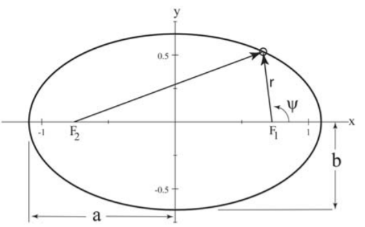
Figure 11.8.1:Bound elliptical orbit.
The minimum value of the orbit occurs when where
This minimum distance is called the periapsis[1].
The maximum distance, which is called the apoapsis, occurs when
Remember that since for bound orbits, the negative signs in equations \text{(11.64)} and \text{(11.65)} lead to . The most bound orbit is a circle having which implies that .
The shape of the elliptical orbit also can be described with respect to the center of the elliptical equivalent orbit by deriving the lengths of the semi-major axis and the semi-minor axis shown in Figure 11.8.1. $$
$$
Remember that the predicted bound elliptical orbit corresponds to the equivalent one-body representation for the two-body motion as illustrated in Figure . This can be transformed to the individual spatial trajectories of the each of the two bodies in an inertial frame.
Kepler’s laws for bound planetary motion
Kepler’s three laws of motion apply to the motion of two bodies in a bound orbit due to the attractive gravitational force for which .
Each planet moves in an elliptical orbit with the sun at one focus
The radius vector, drawn from the sun to a planet, describes equal areas in equal times
The square of the period of revolution about the sun is proportional to the cube of the major axis of the orbit.
Two bodies interacting via the gravitational force, which is a conservative, inverse-square, two-body central force, is best handled using the equivalent orbit representation. The first and second laws were proved in chapters 11.8 and 11.3. That is, the second law is equivalent to the statement that the angular momentum is conserved. The third law can be derived using the fact that the area of an ellipse is
Equations and give that the rate of change of area swept out by the radius vector is
Therefore the period for one revolution is given by the time to sweep out one complete ellipse
This leads to Kepler’s law
Bound orbits occur only for attractive forces for which the force constant is negative, and thus cancel the negative sign in Equation \text{(11.71)}. For example, for the gravitational force .
Note that the reduced mass occurs in Kepler’s law. That is, Kepler’s third law can be written in terms of the actual masses of the bodies to be
In relating the relative periods of the different planets Kepler made the approximation that the mass of the planet is negligible relative to the mass of the sun
The eccentricity of the major planets ranges from for Mercury, to for Venus. The Earth has an eccentricity of with miles and miles. On the other hand, for Halley’s comet, that is, the radius vector ranges from 0.6 to 18 times the radius of the orbit of the Earth.
The orbit energy can be derived by substituting the eccentricity, given by Equation \text{(11.62)}, into the semi-major axis length given by Equation \text{(11.66)}, which leads to the center-of-mass energy of
However, the Hamiltonian, given by equation , implies that is
For the simple case of a circular orbit, then the velocity equals
For a circular orbit, the drag on a satellite lowers the total energy resulting in a decrease in the radius of the orbit and a concomitant increase in velocity. That is, when the orbit radius is decreased, part of the gain in potential energy accounts for the work done against the drag, and the remaining part goes towards increase of the kinetic energy. Also note that, as predicted by the Virial Theorem, the kinetic energy always is half the potential energy for the inverse square law force.
Unbound orbits
Attractive inverse-square central forces lead to hyperbolic orbits for for which , that is, the orbit is unbound. In addition, the orbits always are unbound for a repulsive force since is positive as is the kinetic energy , thus . The radial orbit equation for either an attractive or a repulsive force is
For a repulsive force is positive and always is positive. Therefore to ensure that remain positive the bracket term must be negative. That is
For an attractive force is negative and since is positive then the bracket term must be positive to ensure that is positive. That is,
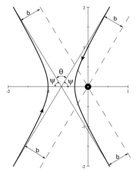
Figure 11.8.2:Hyperbolic two-body orbits for a repulsive (left) and attractive (right) inverse-square, central two-body forces. Both orbits have the angular momentum vector pointing upwards out of the plane of the orbit
Figure 11.8.2 shows both branches of the hyperbola for a given angle for the equivalent two-body orbits where the center of force is at the origin. For an attractive force, the center of force is at the interior focus of the hyperbola, whereas for a repulsive force the center of force is at the exterior focus. For a given value of the asymptotes of the orbits both are displaced by the same impact parameter from parallel lines passing through the center of force. The scattering angle, between the outgoing direction of the scattered body and the incident direction, is designated to be which is related to the angle by .
Eccentricity vector
Two-bodies interacting via a conservative two-body central force have two invariant first-order integrals, namely the conservation of energy and the conservation of angular momentum. For the special case of the inverse-square law, there is a third invariant of the motion, which Hamilton called the eccentricity vector[2], that unambiguously defines the orientation and direction of the major axis of the elliptical orbit. It will be shown that the angular momentum plus the eccentricity vector completely define the plane and orientation of the orbit for a conservative inverse-square law central force.
Newton’s second law for a central force can be written in the form
Note that the angular moment is conserved for a central force, that is . Therefore the time derivative of the product reduces to
This can be simplified using the fact that
thus
This allows Equation \text{(11.80)} to be reduced to
Assume the special case of the inverse-square law, Equation \text{(11.52)}, then the central force Equation \text{(11.83)} reduces to
or
Define the eccentricity vector as
then Equation \text{(11.85)} corresponds to
This is a statement that the eccentricity vector is a constant of motion for an inverse-square, central force.
The definition of the eccentricity vector and angular momentum vector implies a zero scalar product,
Thus the eccentricity vector and angular momentum are mutually perpendicular, that is, is in the plane of the orbit while is perpendicular to the plane of the orbit. The eccentricity vector , always points along the major axis of the ellipse from the focus to the periapsis as illustrated on the left side in Figure 11.8.3. As a consequence, the two orthogonal vectors and completely define the plane of the orbit, plus the orientation of the major axis of the Kepler orbit, in this plane. The three vectors , , and obey the triangle rule as illustrated in the left side of Figure 11.8.3.
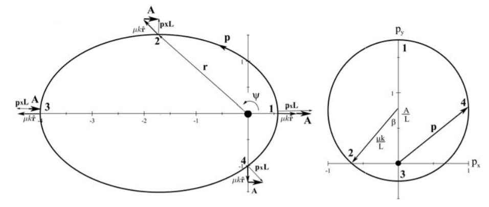
Figure 11.8.3:The elliptical trajectory and eccentricity vector for two bodies interacting via the inverse-square, central force for eccentricity . The left plot shows the elliptical spatial trajectory where the semi-major axis is assumed to be on the -axis and the angular momentum , is out of the page. The force center is at one focus of the ellipse. The vector coupling relation is illustrated at four points on the spatial trajectory. The right plot is a hodograph of the linear momentum for this trajectory. The periapsis is denoted by the number and the apoapsis is marked as on both plots. Note that the eccentricity vector is a constant that points parallel to the major axis towards the perapsis.
Hamilton noted the direct connection between the eccentricity vector and the eccentricity of the conic section orbit. This can be shown by considering the scalar product
Note that the triple scalar product can be permuted to give
Inserting Equation \text{(11.90)} into \text{(11.89)} gives
Note that equations \text{(11.63)} and \text{(11.91)} are identical if . This implies that the eccentricity and are related by
where is defined to be negative for an attractive force. The relation between the eccentricity and total center-of-mass energy can be used to rewrite Equation \text{(11.62)} in the form
The combination of the eccentricity vector and the angular momentum vector completely specifies the orbit for an inverse square-law central force. The trajectory is in the plane perpendicular to the angular momentum vector , while the eccentricity, plus the orientation of the orbit, both are defined by the eccentricity vector . The eccentricity vector and angular momentum vector each have three independent coordinates, that is, these two vector invariants provide six constraints, while the scalar invariant energy adds one additional constraint. The exact location of the particle moving along the trajectory is not defined and thus there are only five independent coordinates governed by the above seven constraints. Thus the eccentricity vector, angular momentum, and center-of-mass energy are related by the two equations \text{(11.88)} and \text{(11.93)}.
Noether’s theorem states that each conservation law is a manifestation of an underlying symmetry. Identification of the underlying symmetry responsible for the conservation of the eccentricity vector is elucidated using Equation \text{(11.86)} to give
Take the scalar product
Choose the angular momentum to be along the -axis, that is, , and, since and are perpendicular to , then and are in the plane. Assume that the semimajor axis of the elliptical orbit is along the -axis, then the locus of the momentum vector on a momentum hodograph has the equation
Equation \text{(11.96)} implies that the locus of the momentum vector is a circle of radius with the center displaced from the origin at coordinates as shown by the momentum hodograph on the right side of an Figure 11.8.3. The angle and eccentricity are related by,
The circular orbit is centered at the origin for , and thus the magnitude is a constant around the whole trajectory.
The inverse-square, central, two-body, force is unusual in that it leads to stable closed bound orbits because the radial and angular frequencies are degenerate, i.e. In momentum space, the locus of the linear momentum vector is a perfect circle which is the underlying symmetry responsible for both the fact that the orbits are closed, and the invariance of the eccentricity vector. Mathematically this symmetry for the Kepler problem corresponds to the body moving freely on the boundary of a four-dimensional sphere in space and momentum. The invariance of the eccentricity vector is a manifestation of the special property of the inverse-square, central force under certain rotations in this four-dimensional space; this symmetry is an example of a hidden symmetry.
11.9: Isotropic, linear, two-body, central force
Closed orbits occur for the two-dimensional linear oscillator when is a rational fraction as discussed in chapter 3.3. Bertrand’s Theorem states that the linear oscillator, and the inverse-square law (Kepler problem), are the only two-body central forces that have single-valued, stable, closed orbits of the coupled radial and angular motion. The invariance of the eccentricity vector was the underlying symmetry leading to single-valued, stable, closed orbits for the Kepler problem. It is interesting to explore the symmetry that leads to stable closed orbits for the harmonic oscillator. For simplicity, this discussion will restrict discussion to the isotropic, harmonic, two-body, central force where , for which the two-body, central force is linear
where corresponds to a repulsive force and to an attractive force. This isotropic harmonic force can be expressed in terms of a spherical potential where
Since this is a central two-body force, both the equivalent one-body representation, and the conservation of angular momentum, are equally applicable to the harmonic two-body force. As discussed in section 11.3, since the two-body force is central, the motion is confined to a plane, and thus the Lagrangian can be expressed in polar coordinates. In addition, since the force is spherically symmetric, then the angular momentum is conserved. The orbit solutions are conic sections as described in chapter 11.7. The shape of the orbit for the harmonic two-body central force can be derived using either polar or cartesian coordinates as illustrated below.
Polar coordinates
The origin of the equivalent orbit for the harmonic force will be found to be at the center of an ellipse, rather than the foci of the ellipse as found for the inverse square law. The shape of the orbit can be defined using a Binet differential orbit equation that employs the transformation
Then
The chain rule gives that
Substitute this into the Hamiltonian equation , gives
Rearranging this equation gives
Addition of a constant to both sides of the equation completes the square
The right-hand side of Equation \text{(11.105)} is a constant. The solution of \text{(11.105)} must be a sine or cosine function with polar angle . That is
That is,
Equation \text{(11.107)} corresponds to a closed orbit centered at the origin of the elliptical orbit as illustrated in Figure 11.9.1. The eccentricity of this closed orbit is given by
Equations , give that the eccentricity is related to the semi-major and semi-minor axes by
Note that for a repulsive force , then leading to unbound hyperbolic or parabolic orbits centered on the origin. An attractive force, allows for bound elliptical, as well as unbound parabolic and hyperbolic orbits.
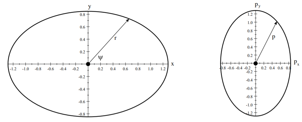
Figure 11.9.1:The elliptical equivalent trajectory for two bodies interacting via the linear, central force for eccentricity . The left plot shows the elliptical spatial trajectory where the semi-major axis is assumed to be on the -axis and the angular momentum , is out of the page. The force center is at the center of the ellipse. The right plot is a hodograph of the linear momentum for this trajectory.
Cartesian coordinates
The isotropic harmonic oscillator, expressed in terms of cartesian coordinates in the plane of the orbit, is separable because there is no direct coupling term between the and motion. That is. the center-of-mass Lagrangian in the plane separates into independent motion for and .
Solutions for the independent coordinates, and their corresponding momenta, are
where . Therefore
where
For a phase difference this equation describes an ellipse centered at the origin which agrees with Equation \text{(11.107)} that was derived using polar coordinates.
The two normal modes of the isotropic harmonic oscillator are degenerate, therefore are equally good normal modes with two corresponding total energies, , while the corresponding angular momentum points in the direction. $$
$$
Figure 11.9.1 shows the closed elliptical equivalent orbit plus the corresponding momentum hodograph for the isotropic harmonic two-body central force. Figures and 11.9.1 contrast the differences between the elliptical orbits for the inverse-square force, and those for the harmonic two-body central force. Although the orbits for bound systems with the harmonic two-body force, and the inverse-square force, both lead to elliptical bound orbits, there are important differences. Both the radial motion and momentum are two valued per cycle for the reflection-symmetric harmonic oscillator, whereas the radius and momentum have only one maximum and one minimum per revolution for the inverse-square law. Although the inverse-square, and the isotropic, harmonic, two-body central forces both lead to closed bound elliptical orbits for which the angular momentum is conserved and the orbits are planar, there is another important difference between the orbits for these two interactions. The orbit equation for the Kepler problem is expressed with respect to a foci of the elliptical equivalent orbit, as illustrated in Figure , whereas the orbit equation for the isotropic harmonic oscillator orbit isexpressed with respect to the center of the ellipse as illustrated in Figure 11.9.1.
Symmetry tensor 
The invariant vectors and provide a complete specification of the geometry of the bound orbits for the inverse square-law Kepler system. It is interesting to search for a similar invariant that fully specifies the orbits for the isotropic harmonic central force. In contrast to the Kepler problem, the harmonic force center is at the center of the elliptical orbit, and the orbit is reflection symmetric with the radial and angular frequencies related by . Since the orbit is reflection-symmetric, the orientation of the major axis of the orbit cannot be uniquely specified by a vector. Therefore, for the harmonic interaction it is necessary to specify the orientation of the principal axis by the symmetry tensor. The symmetry of the isotropic harmonic, two-body, central force leads to the symmetry tensor which is an invariant of the motion analogous to the eccentricity vector . Like a rotation matrix, the symmetry tensor defines the orientation, but not direction, of the major principal axis of the elliptical orbit. In the plane of the polar orbit the symmetry tensor reduces to a matrix having matrix elements defined to be,
The diagonal matrix elements , and are constants of motion. The off-diagonal term is given by
The terms on the right-hand side of Equation \text{(11.119)} all are constants of motion, therefore also is a constant of motion. Thus the symmetry tensor can be reduced to a symmetry tensor for which all the matrix elements are constants of motion, and the trace of the symmetry tensor is equal to the total energy.
In summary, the inverse-square, and harmonic oscillator two-body central interactions both lead to closed, elliptical equivalent orbits, the plane of which is perpendicular to the conserved angular momentum vector. However, for the inverse-square force, the origin of the equivalent orbit is at the focus of the ellipse and , whereas the origin is at the center of the ellipse and for the harmonic force. As a consequence, the elliptical orbit is reflection symmetric for the harmonic force but not for the inverse square force. The eccentricity vector and symmetry tensor both specify the major axes of these elliptical orbits, the plane of which are perpendicular to the angular momentum vector. The eccentricity vector, and the symmetry tensor, both are directly related to the eccentricity of the orbit and the total energy of the two-body system. Noether’s theorem states that the invariance of the eccentricity vector and symmetry tensor, plus the corresponding closed orbits, are manifestations of underlying symmetries. The dynamical symmetry underlies the invariance of the symmetry tensor, whereas the dynamical symmetry underlies the invariance of the eccentricity vector. These symmetries lead to stable closed elliptical bound orbits only for these two specific two-body central forces, and not for other two-body central forces.
11.10: Closed-orbit Stability
Bertrand’s theorem states that the linear oscillator and the inverse-square law are the only two-body, central forces for which all bound orbits are single-valued, and stable closed orbits. The stability of closed orbits can be illustrated by studying their response to perturbations. For simplicity, the following discussion of stability will focus on circular orbits, but the general principles are the same for elliptical orbits.
A circular orbit occurs whenever the attractive force just balances the effective ”centrifugal force” in the rotating frame. This can occur for any radial functional form for the central force. The effective potential, equation will have a stationary point when
that is, when
This is equivalent to the statement that the net force is zero. Since the central attractive force is given by
then the stationary point occurs when
This is the so-called centrifugal force in the rotating frame. The Hamiltonian, equation , gives that
For a circular orbit that is
A stable circular orbit is possible if both equations \text{(11.121)} and \text{(11.125)} are satisfied. Such a circular orbit will be a stable orbit at the minimum when
Examples of stable and unstable orbits are shown in Figure 11.10.1.
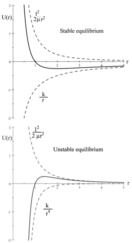
Figure 11.10.1:Stable and unstable effective central potentials. The repulsive centrifugal and the attractive potentials are shown dashed. The solid curve is the effective potential.
Stability of a circular orbit requires that
which can be written in terms of the central force for a stable orbit as
If the attractive central force can be expressed as a power law
then stability requires
or
Stable equivalent orbits will undergo oscillations about the stable orbit if perturbed. To first order, the restoring force on a bound reduced mass is given by
To the extent that this linear restoring force dominates over higher-order terms, then a perturbation of the stable orbit will undergo simple harmonic oscillations about the stable orbit with angular frequency
The above discussion shows that a small amplitude radial oscillation about the stable orbit with amplitude will be of the form
The orbit will be closed if the product of the oscillation frequency and the orbit period is an integer value.
The fact that planetary orbits in the gravitational field are observed to be closed is strong evidence that the gravitational force field must obey the inverse square law. Actually there are small precessions of planetary orbits due to perturbations of the gravitational field by bodies other than the sun, and due to relativistic effects. Also the gravitational field near the earth departs slightly from the inverse square law because the earth is not a perfect sphere, and the field does not have perfect spherical symmetry. The study of the precession of satellites around the earth has been used to determine the oblate quadrupole and slight octupole (pear shape) distortion of the shape of the earth.
The most famous test of the inverse square law for gravitation is the precession of the perihelion of Mercury. If the attractive force experienced by Mercury is of the form
where is small, then it can be shown that, for approximate circular orbitals, the perihelion will advance by a small angle per orbit period. That is, the precession is zero if , corresponding to an inverse square law dependence which agrees with Bertrand’s theorem. The position of the perihelion of Mercury has been measured with great accuracy showing that, after correcting for all known perturbations, the perihelion advances by seconds of arc per century, that is radians per revolution. This corresponds to which is small but still significant. This precession remained a puzzle for many years until 1915 when Einstein predicted that one consequence of his general theory of relativity is that the planetary orbit of Mercury should precess at 43 seconds of arc per century, which is in remarkable agreement with observations.
11.11: The Three-Body Problem
Two bodies interacting via conservative central forces can be solved analytically for the inverse square law and the Hooke’s law radial dependences as already discussed. Central forces that have other radial dependences for the equations of motion may not be expressible in terms of simple functions, nevertheless the motion always can be given in terms of an integral. For a gravitational system comprising bodies that are interacting via the two-body central gravitational force, then the equations of motion can be written as
Even when all the bodies are interacting via two-body central forces, the problem usually is insoluble in terms of known analytic integrals. Newton first posed the difficulty of the three-body Kepler problem which has been studied extensively by mathematicians and physicists. No known general analytic integral solution has been found. Each body for the -body system has 6 degrees of freedom, that is, 3 for position and 3 for momentum. The center-of-mass motion can be factored out, therefore the center-of-mass system for the -body system has degrees of freedom after subtraction of 3 degrees for location of the center of mass, 3 for the linear momentum of the center of mass, 3 for rotation of the center of mass, and 1 for the total energy of the system. Thus for there are degrees of freedom for the two-body system for which the Kepler approach takes to be and For there are 8 degrees of freedom in the center of mass system that have to be determined.
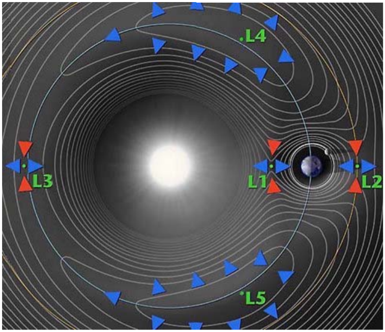
Figure 11.11.1:A contour plot of the effective potential for the Sun-Earth gravitational system in the rotating frame where the Sun and Earth are stationary. The 5 Lagrange points are saddle points where the net force is zero. (Figure created by NASA)
Numerical solutions to the three-body problem can be obtained using successive approximation or perturbation methods in computer calculations. The problem can be simplified by restricting the motion to either of following two approximations:
1) Planar approximation
This approximation assumes that the three masses move in the same plane, that is, the number of degrees of freedom are reduced from 8 to 6 which simplifies the numerical solution.
2) Restricted three-body approximation
The restricted three-body approximation assumes that two of the masses are large and bound while the third mass is negligible such that the perturbation of the motion of the larger two by the third body is negligible. This approximation essentially reduces the system to a two body problem in order to calculate the gravitational fields that act on the third much lighter mass.
Euler and Lagrange showed that the restricted three-body system has five points at which the combined gravitational attraction plus centripetal force of the two large bodies cancel. These are called the Lagrange points and are used for parking satellites in stable orbits with respect to the Earth-Moon system, or with respect to the Sun-Earth system. Figure 11.11.1 illustrates the five Lagrange points for the Earth-Sun system. Only two of the Lagrange points, and lead to stable orbits. Note that these Lagrange points are fixed with respect to the Earth-Sun system which rotates with respect to inertial coordinate frames. The 1900’s discovery of the Trojan asteroids at the and Lagrange points of the Sun-Jupiter system confirmed the Lagrange predictions.
Poincaré showed that the motion of a light mass bound to two heavy bodies can exhibit extreme sensitivity to initial conditions as well as characteristics of chaos. Solution of the three-body problem has remained a largely unsolved problem since Newton identified the difficulties involved.
11.12: Two-body Scattering
Two moving bodies, that are interacting via a central force, scatter when the force is repulsive, or when an attractive system is unbound. Two-body scattering of bodies is encountered extensively in the fields of astronomy, atomic, nuclear, and particle physics. The probability of such scattering is most conveniently expressed in terms of scattering cross sections defined below.
Total two-body scattering cross section
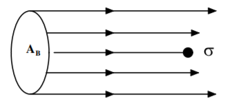
Figure 11.12.1:Scattering probability for an incident beam of cross sectional area A by a target body of cross sectional area .
The concept of scattering cross section for two-body scattering is most easily described for the total two-body cross section. The probability that a beam of incident point particles/second, distributed over a cross sectional area will hit a single solid object, having a cross sectional area is given by the ratio of the areas as illustrated in Figure 11.12.1. That is,
where it is assumed that For a spherical target body of radius , the cross section The scattering probability is proportional to the cross section which is the cross section of the target body perpendicular to the beam; thus has the units of area.
Since the incident beam of incident point particles/second, has a cross sectional area , then it will have an areal density given by
The number of beam particles scattered per second by this single target scatterer equals
Thus the cross section for scattering by this single target body is
Realistically one will have many target scatterers in the target and the total scattering probability increases proportionally to the number of target scatterers. That is, for a target comprising an areal density of target bodies per unit area of the incident beam, then the number scattered will increase proportional to the target areal density That is, there will be scattering bodies that interact with the beam assuming that the target has a larger area than the beam. Thus the total number scattered per second by a target that comprises multiple scatterers is
Note that this is independent of the cross sectional area of the beam assuming that the target area is larger than that of the beam. That is, the number scattered per second is proportional to the cross section times the product of the number of incident particles per second, and the areal density of target scatterers, . Typical cross sections encountered in astrophysics are , in atomic physics: , and in nuclear physics; [3]
N. B., the above proof assumed that the target size is larger than the cross sectional area of the incident beam. If the size of the target is smaller than the beam, then is replaced by the areal density/s of the beam and is replaced by the number of target particles and the cross-sectional size of the target cancels.
Differential two-body scattering cross section
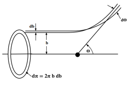
Figure 11.12.2:The equivalent one-body problem for scattering of a reduced mass by a force center in the center of mass system.
The differential two-body scattering cross section gives much more detailed information of the scattering force than does the total cross section because of the correlation between the impact parameter and the scattering angle. That is, a measurement of the number of beam particles scattered into a given solid angle as a function of scattering angles probes the radial form of the scattering force.
The differential cross section for scattering of an incident beam by a single target body into a solid angle at scattering angles is defined to be
where the right-hand side is the ratio of the number scattered per target nucleus into solid angle to the incident beam intensity .
Similar reasoning used to derive Equation \text{(11.137)} leads to the number of beam particles scattered into a solid angle for beam particles incident upon a target with areal density is
Consider the equivalent one-body system for scattering of one body by a scattering force center in the center of mass. As shown in figures and 11.12.2, the perpendicular distance between the center of force of the two body system and trajectory of the incoming body at infinite distance is called the impact parameter . For a central force the scattering system has cylindrical symmetry, therefore the solid angle can be integrated over the azimuthal angle to give
For the inverse-square, two-body, central force there is a one-to-one correspondence between impact parameter and scattering angle for a given bombarding energy. In this case, assuming conservation of flux means that the incident beam particles passing through the impact-parameter annulus between and must equal the number passing between the corresponding angles and That is, for an incident beam flux of the number of particles per second passing through the annulus is
The modulus is used to ensure that the number of particles is always positive. Thus
Impact parameter dependence on scattering angle
If the function is known, then it is possible to evaluate which can be used in Equation \text{(11.141)} to calculate the differential cross section. A simple and important case to consider is two-body elastic scattering for the inverse-square law force such as the Coulomb or gravitational forces. To avoid confusion in the following discussion, the center-of-mass scattering angle will be called while the angle used to define the hyperbolic orbits in the discussion of trajectories for the inverse square law, will be called .
In chapter 11.8 the equivalent one-body representation gave that the radial distance for a trajectory for the inverse square law is given by
Note that closest approach occurs when while for the bracket must equal zero, that is
The polar angle is measured with respect to the symmetry axis of the two-body system which is along the line of distance of closest approach as shown in Figure . The geometry and symmetry show that the scattering angle is related to the trajectory angle by
Equation gives that
Since
then the scattering angle can be written as.
Let , then
For the repulsive inverse square law
where is taken to be positive for a repulsive force. Thus the scattering angle relation becomes
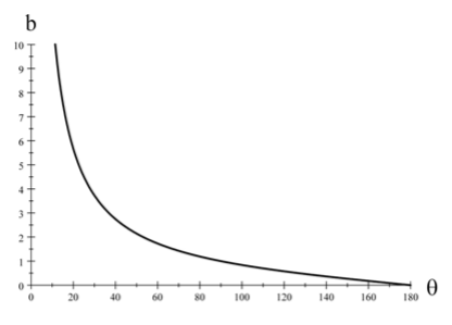
Figure 11.12.3:Impact parameter dependence on scattering angle for Rutherford scattering.
The solution of this equation is given by equation to be
where the eccentricity
For then, as shown previously,
Therefore
that is, the impact parameter is given by the relation
Thus, for an inverse-square law force, the two-body scattering has a one-to-one correspondence between impact parameter and scattering angle as shown schematically in Figure 11.12.3.
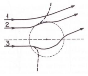
Figure 11.12.4:Classical trajectories for scattering to a given angle by the repulsive Coulomb field plus the attractive nuclear field for three different impact parameters. Path 1 is pure Coulomb. Paths 2 and 3 include Coulomb plus nuclear interactions. The dashed parts of trajectories 2 and 3 correspond to only the Coulomb force acting, i.e. zero nuclear force
If is negative, which corresponds to an attractive inverse square law, then one gets the same relation between impact parameter and scattering angle except that the sign of the impact parameter is opposite. This means that the hyperbolic trajectory has an interior rather than exterior focus. That is, the trajectory partially orbits around the center of force rather than being repelled away.
Note that for then
which is what you would expect from equating the incident kinetic energy to the potential energy at the distance of closest approach.
For scattering of two nuclei by the repulsive Coulomb force, if the impact parameter becomes small enough, the attractive nuclear force also acts leading to impact-parameter dependent effective potentials illustrated in Figure 11.12.4. Trajectory 1 does not overlap the nuclear force and thus is pure Coulomb. Trajectory 2 interacts at the periphery of the nuclear potential and the trajectory deviates from pure Coulomb shown dashed. Trajectory 3 passes through the interior of the nuclear potential. These three trajectories all can lead to the same scattering angle and thus there no longer is a one-to-one correspondence between scattering angle and impact parameter.
Rutherford scattering
Two models of the nucleus evolved in the 1900’s, the Rutherford model assumed electrons orbiting around a small nucleus like planets around the sun, while J.J. Thomson’s ”plum-pudding” model assumed the electrons were embedded in a uniform sphere of positive charge the size of the atom. When Rutherford derived his classical formula in 1911 he realized that it can be used to determine the size of the nucleus since the electric field obeys the inverse square law only when outside of the charged spherical nucleus. Inside a uniform sphere of charge the electric field is and thus the scattering cross section will not obey the Rutherford relation for distances of closest approach that are less than the radius of the sphere of negative charge. Observation of the angle beyond which the Rutherford formula breaks down immediately determines the radius of the nucleus.
This cross section assumes elastic scattering by a repulsive two-body inverse-square central force. For scattering of nuclei in the Coulomb potential, the constant is given to be
The cross section, scattering angle and of Equation \text{(11.159)} are evaluated in the center-of-mass coordinate system, whereas usually two-body elastic scattering data involve scattering of the projectiles by a stationary target as discussed in chapter 11.13.
Geiger and Marsden performed scattering of 7.7 MeV particles from a thin gold foil and proved that the differential scattering cross section obeyed the Rutherford formula back to angles corresponding to a distance of closest approach of which is much smaller that the size of the atom. This validated the Rutherford model of the atom and immediately led to the Bohr model of the atom which played such a crucial role in the development of quantum mechanics. Bohr showed that the agreement with the Rutherford formula implies the Coulomb field obeys the inverse square law to small distances. This work was performed at Manchester University, England between 1908 and 1913. It is fortunate that the classical result is identical to the quantal cross section for scattering, otherwise the development of modern physics could have been delayed for many years.
Scattering of very heavy ions, such as Pb, can electromagnetically excite target nuclei. For the Coulomb force the impact parameter and the distance of closest approach, are directly related to the scattering angle by Equation \text{(11.155)}. Thus observing the angle of the scattered projectile unambiguously determines the hyperbolic trajectory and thus the electromagnetic impulse given to the colliding nuclei. This process, called Coulomb excitation, uses the measured angular distribution of the scattered ions for inelastic excitation of the nuclei to precisely and unambiguously determine the Coulomb excitation cross section as a function of impact parameter. This unambiguously determines the shape of the nuclear charge distribution.
11.13: Two-body kinematics
So far the discussion has been restricted to the center-of-momentum system. Actual scattering measurements are performed in the laboratory frame, and thus it is necessary to transform the scattering angle, energies and cross sections between the laboratory and center-of-momentum coordinate frame. In principle the transformation between the center-of-momentum and laboratory frames is straightforward, using the vector addition of the center-of-mass velocity vector and the center-of-momentum velocity vectors of the two bodies. The following discussion assumes non-relativistic kinematics apply.
In chapter 2.8 it was shown that, for Newtonian mechanics, the center-of-mass and center-of-momentum frames of reference are identical. By definition, in the center-of-momentum frame the vector sum of the linear momentum of the incoming projectile, and target, are equal and opposite. That is
Using the center-of-momentum frame, coupled with the conservation of linear momentum, implies that the vector sum of the final momenta of the reaction products, also is zero. That is
An additional constraint is that energy conservation relates the initial and final kinetic energies by
where the value is the energy contributed to the final total kinetic energy by the reaction between the incoming projectile and target. For exothermic reactions, the summed kinetic of the reaction products exceeds the sum of the incoming kinetic energies, while for endothermic reactions, the summed kinetic energy of the reaction products is less than that of the incoming channel.
For two-body kinematics, the following are three advantages to working in the center-of-momentum frame of reference.
The two incident colliding bodies are collinear as are the two final bodies.
The linear momenta for the two colliding bodies are identical in both the incident channel and the outgoing channel.
The total energy in the center-of-momentum coordinate frame is the energy available to the reaction during the collision. The trivial kinetic energy of the center-of-momentum frame relative to the laboratory frame is handled separately.
The kinematics for two-body reactions is easily determined using the conservation of linear momentum along and perpendicular to the beam direction plus the conservation of energy, \text{(11.161)}-\text{(11.163)}. Note that it is common practice to use the term “center-of-mass” rather than “center-of-momentum” in spite of the fact that, for relativistic mechanics, only the center-of-momentum is a meaningful concept.
General features of the transformation between the center-of-momentum and laboratory frames of reference are best illustrated by elastic or inelastic scattering of nuclei where the two reaction products in the final channel are identical to the incident bodies. Inelastic excitation of an excited state energy of in either reaction product corresponds to while elastic scattering corresponds to .
For inelastic scattering, the conservation of linear momenta for the outgoing channel in the center-of-momentum simplifies to
that is, the linear momenta of the two reaction products are equal and opposite.
Assume that the center-of-momentum direction of the scattered projectile is at an angle relative to the direction of the incoming projectile and that the scattered target nucleus is scattered at a center-of-momentum direction . Elastic scattering corresponds to simple scattering for which the magnitudes of the incoming and outgoing projectile momenta are equal, that is, .
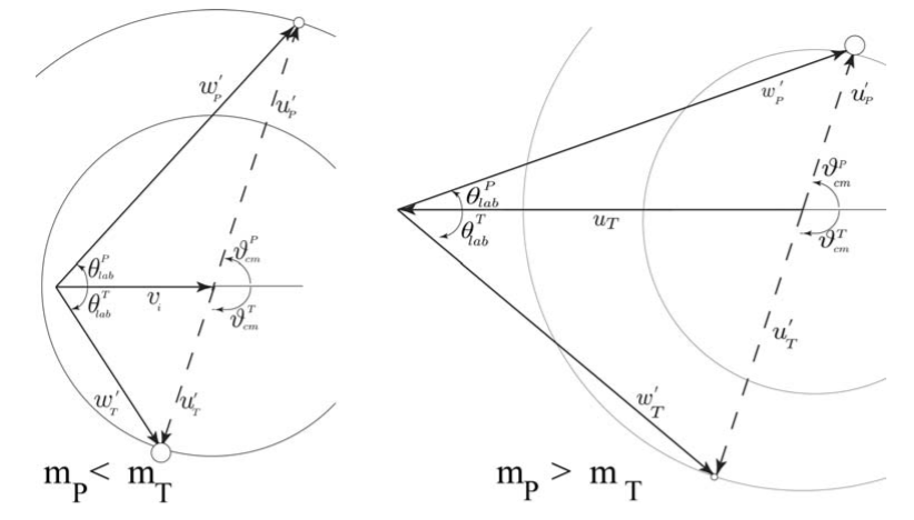
Figure 11.13.1:Vector hodograph of the scattered projectile and target velocities for a projectile, with incident velocity , that is elastically scattered by a stationary target body. The circles show the magnitude of the projectile and target body final velocities in the center of mass. The center-of-mass velocity vectors are shown as dashed lines while the laboratory vectors are shown as solid lines. The left hodograph shows normal kinematics where the projectile mass is less than the target mass. The right hodograph shows inverse kinematics where the projectile mass is greater than the target mass. For elastic scattering .
Velocities
The transformation between the center-of-momentum and laboratory frames requires knowledge of the particle velocities which can be derived from the linear momenta since the particle masses are known. Assume that a projectile, mass , with incident energy in the laboratory frame bombards a stationary target with mass The incident projectile velocity is given by
The initial velocities in the laboratory frame are taken to be
The final velocities in the laboratory frame after the inelastic collision are $$
$$
In the center-of-momentum coordinate system, equation implies that the initial center-of-momentum velocities are $$
$$
It is simple to derive that the final center-of-momentum velocities after the inelastic collision are given by
The energy is defined to be given by
where which is the excitation energy of the final excited states in the outgoing channel.
Angles
The angles of the scattered recoils are written as
and
where is the center-of-mass (center-of-momentum) scattering angle.
Figure 11.13.1 shows that the angle relations between the laboratory and center of momentum frames for the scattered projectile are connected by
where
and is the energy per nucleon on the incident projectile.
Equation \text{(11.169)} can be rewritten as
Another useful relation from Equation \text{(11.169)} gives the center-of-momentum scattering angle in terms of the laboratory scattering angle.
This gives the difference in angle between the lab scattering angle and the center-of-momentum scattering angle. Be careful with this relation since is two-valued for inverse kinematics corresponding to the two possible signs for the solution.
The angle relations between the lab and center-of-momentum for the recoiling target nucleus are connected by
That is
where
Note that is the same under interchange of the two nuclei at the same incident energy/nucleon, and that is always larger than or equal to unity since is negative. For elastic scattering which gives
For the target recoil Equation \text{(11.173)} can be rewritten as
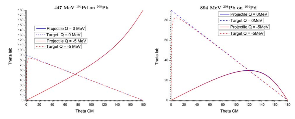
Figure 11.13.2:The kinematic correlation of the laboratory and center-of-mass scattering angles of the recoiling projectile and target nuclei for scattering for 4.3 /nucleon Pd on Pb (left) and for the inverse 4.3 /nucleon Pb on Pd (right). The projectile scattering angles are shown by solid lines while the recoiling target angles are shown by dashed lines. The blue curves correspond to elastic scattering, that is while the red curves correspond to inelastic scattering with .
Velocity vector hodographs provide useful insight into the behavior of the kinematic solutions. As shown in Figure 11.13.1, in the center-of-momentum frame the scattered projectile has a fixed final velocity , that is, the velocity vector describes a circle as a function of . The vector addition of this vector and the velocity of the center-of-mass vector gives the laboratory frame velocity . Note that for normal kinematics, where then leading to a monotonic one-to-one mapping of the center-of-momentum angle and . However, for inverse kinematics, where then leading to two valued solutions at any fixed laboratory scattering angle .
Billiard ball collisions are an especially simple example where the two masses are identical and the collision is essentially elastic. Then essentially , and , that is, the angle between the scattered billiard balls is .
Both normal and inverse kinematics are illustrated in Figure 11.13.2 which shows the dependence of the projectile and target scattering angles in the laboratory frame as a function of center-of-momentum scattering angle for the Coulomb scattering of Pd by Pb, that is, for a mass ratio of . Both normal and inverse kinematics are shown for the same bombarding energy of 4.3 for elastic scattering and for inelastic scattering with a -value of .
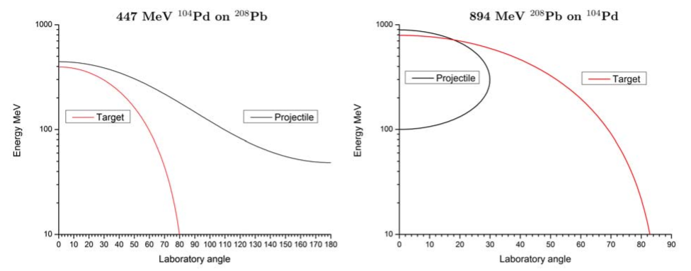
Figure 11.13.3:Recoil energies, in , versus laboratory scattering angle, shown on the left for scattering of 447 Pd by Pb with , and shown on the right for scattering of 894 Pb on Pd with .
Since then Equation \text{(11.173)} implies that Since is always larger than or equal to unity there is a maximum scattering angle in the laboratory frame for the recoiling target nucleus given by
For elastic scattering since for both 894 Pb bombarding Pd, and the inverse reaction using a 447 Pd beam scattered by a Pb target. A -value of -5 gives which implies a maximum scattering angle of for both 894 Pb bombarding Pd, and the inverse reaction of a 447 Pd beam scattered by a Pb target. As a consequence there are two solutions for for any allowed value of as illustrated in Figure 11.13.3.
Since then equation implies that For a 447 Pd beam scattered by a Pb target , thus for elastic scattering which implies that there is no upper bound to . This leads to a one-to-one correspondence between and for normal kinematics. In contrast, the projectile has a maximum scattering angle in the laboratory frame for inverse kinematics since leading to an upper bound to given by
For elastic scattering implying . In addition to having a maximum value for , when also there are two solutions for for any allowed value of . For the example of 894 Pb bombarding Hf leads to a maximum projectile scattering angle of for elastic scattering and for
Kinetic energies
The initial total kinetic energy in the center-of-momentum frame is
The final total kinetic energy in the center-of-momentum frame is
In the laboratory frame the kinetic energies of the scattered projectile and recoiling target nucleus are given by
where and are the center-of-mass scattering angles respectively for the scattered projectile and target nuclei.
For the chosen incident energies the normal and inverse reactions give the same center-of-momentum energy of 298 which is the energy available to the interaction between the colliding nuclei. However, the kinetic energy of the center-of-momentum is for normal kinematics and for inverse kinematics. This trivial center-of-momentum kinetic energy does not contribute to the reaction. Note that inverse kinematics focuses all the scattered nuclei into the forward hemisphere which reduces the required solid angle for recoil-particle detection.
Solid angles
The laboratory-frame solid angles for the scattered projectile and target are taken to be and respectively, while the center-of-momentum solid angles are and respectively. The Jacobian relating the solid angles is
These can be used to transform the calculated center-of-momentum differential cross sections to the laboratory frame for comparison with measured values. Note that relative to the center-of-momentum frame, the forward focusing increases the observed differential cross sections in the forward laboratory frame and decreases them in the backward hemisphere.
Exploitation of two-body kinematics
Computing the above non-trivial transform relations between the center-of-mass and laboratory coordinate frames for two-body scattering is used extensively in many fields of physics. This discussion has assumed non-relativistic two-body kinematics. Relativistic two-body kinematics encompasses non-relativistic kinematics as discussed in chapter 17.4. Many computer codes are available that can be used for making either non-relativistic or relativistic transformations.
It is stressed that the underlying physics for two interacting bodies is identical irrespective of whether the reaction is observed in the center-of-mass or the laboratory coordinate frames. That is, no new physics is involved in the kinematic transformation. However, the transformation between these frames can dramatically alter the angles and velocities of the observed scattered bodies which can be beneficial for experimental detection. For example, in heavy-ion nuclear physics the projectile and target nuclei can be interchanged leading to very different velocities and scattering angles in the laboratory frame of reference. This can greatly facilitate identification and observation of the velocities vectors of the scattered nuclei. In high-energy physics it is advantageous to collide beams having identical, but opposite, linear momentum vectors, since then the laboratory frame is the center-of-mass frame, and the energy required to accelerate the colliding bodies is minimized.
11.E: Conservative two-body Central Forces (Exercises)
Listed below are several statements concerning central force motion. For each statement, give the reason for why the statement is true. If a statement is only true in certain situations, then explain when it holds and when it doesn’t. The system referred to below consists of mass
located at
and mass
located at
.
The potential energy of the system depends only on the difference , not on and separately.
The potential energy of the system depends only on the magnitude of , not the direction.
It is possible to choose an inertial reference frame in which the center of mass of the system is at rest.
The total energy of the system is conserved.
The total angular momentum of the system is conserved.
A particle of mass moves in a potential .
Given the constant , find an implicit equation for the radius of the circular orbit. A circular orbit at is possible if
where is the effective potential.
What is the largest value of for which a circular orbit exists? What is the value of the effective potential at this critical orbit?
A particle of mass is observed to move in a spiral orbit given by the equation , where is a constant. Is it possible to have such an orbit in a central force field? If so, determine the form of the force function.
The interaction energy between two atoms of mass is given by the Lennard-Jones potential,
Determine the Lagrangian of the system where and are the positions of the first and second mass, respectively.
Rewrite the Lagrangian as a one-body problem in which the center-of-mass is stationary.
Determine the equilibrium point and show that it is stable.
Determine the frequency of small oscillations about the stable point.
Consider two bodies of mass in circular orbit of radius , attracted to each other by a force , where is the distance between the masses.
Determine the Lagrangian of the system in the center-of-mass frame (Hint: a one-body problem subject to a central force).
Determine the angular momentum. Is it conserved?
Determine the equation of motion in in terms of the angular momentum and .
Expand your result in (c) about an equilibrium radius and show that the condition for stability is,
Consider two charges of equal magnitude connected by a spring of spring constant in circular orbit. Can the charges oscillate about some equilibrium? If so, what condition must be satisfied?
Consider a mass in orbit around a mass , which is subject to a force , where is the distance between the masses. Show that the eccentricity vector is conserved.
Show that the areal velocity is constant for a particle moving under the influence of an attractive force given by . Calculate the time averages of the kinetic and potential energies and compare with the results of the virial theorem.
Assume that the Earth’s orbit is circular and that the Sun’s mass suddenly decreases by a factor of two.
What orbit will the earth then have?
Will the Earth escape the solar system?
Discuss the motion of a particle in a central inverse-square-law force field for a superimposed force whose magnitude is inversely proportional to the cube of the distance from the particle to force center; that is
Show that the motion is described by a precessing ellipse. Consider the cases a) , b) , c) where is the angular momentum and the reduced mass.
A communications satellite is in a circular orbit around the earth at a radius and velocity . A rocket accidentally fires quite suddenly, giving the rocket an outward velocity in addition to its original tangential velocity .
Calculate the ratio of the new energy and angular momentum to the old.
Describe the subsequent motion of the satellite and plot , , the net effective potential, and after the rocket fires.
Two identical point objects, each of mass are bound by a linear two-body force where is the vector distance between the two point objects. The two point objects each slide on a horizontal frictionless plane subject to a vertical gravitational field . The two-body system is free to translate, rotate and oscillate on the surface of the frictionless plane.
Derive the Lagrangian for the complete system including translation and relative motion.
Use Noether’s theorem to identify all constants of motion.
Use the Lagrangian to derive the equations of motion for the system.
Derive the generalized momenta and the corresponding Hamiltonian.
Derive the period for small amplitude oscillations of the relative motion of the two masses.
A bound binary star system comprises two spherical stars of mass and bound by their mutual gravitational attraction. Assume that the only force acting on the stars is their mutual gravitation attraction and let be the instantaneous separation distance between the centers of the two stars where is much larger than the sum of the radii of the stars.
Show that the two-body motion of the binary star system can be represented by an equivalent one-body system and derive the Lagrangian for this system.
Show that the motion for the equivalent one-body system in the center of mass frame lies entirely in a plane and derive the angle between the normal to the plane and the angular momentum vector.
Show whether is a constant of motion and whether it equals the total energy.
It is known that a solution to the equation of motion for the equivalent one-body orbit for this gravitational force has the form
and that the angular momentum is a constant of motion . Use these to prove that the attractive force leading to this bound orbit is
where must be negative.
When performing the Rutherford experiment, Geiger and Marsden scattered 7.7 He particles (alpha particles) from U at a scattering angle in the laboratory frame of . Derive the following observables as measured in the laboratory frame.
The recoil scattering angle of the U in the laboratory frame.
The scattering angles of the He and U in the center-of-mass frame
The kinetic energies of the He and U in the laboratory frame
The impact parameter
The distance of closest approach
11.S: Conservative two-body Central Forces (Summary)
This chapter has focused on the classical mechanics of bodies interacting via conservative, two-body, central interactions. The following are the main topics presented in this chapter.
Equivalent one-body representation for two bodies interacting via a central interaction
The equivalent one-body representation of the motion of two bodies interacting via a two-body central interaction greatly simplifies solution of the equations of motion. The position vectors and are expressed in terms of the center-of-mass vector plus total mass while the position vector , plus associated reduced mass describe the relative motion of the two bodies in the center of mass. The total Lagrangian then separates into two independent parts
where the center-of-mass Lagrangian is
Equations , and can be used to derive the actual spatial trajectories of the two bodies expressed in terms of and , from the relative equations of motion, written in terms of and , for the equivalent one-body solution..
Angular momentum
Noether’s theorem shows that the angular momentum is conserved if only a spherically-symmetric two-body central force acts between the interacting two bodies. The plane of motion is perpendicular to the angular momentum vector and thus the Lagrangian can be expressed in polar coordinates as
Differential orbit equation of motion
The Binet transformation allows the center-of-mass Lagrangian for a central force to be used to express the differential orbit equation for the radial motion as
The Lagrangian, and the Hamiltonian all were used to derive the equations of motion for two bodies interacting via a two-body, conservative, central interaction. The general features of the conservation of angular momentum and conservation of energy for a two-body, central potential were presented.
Inverse-square, two-body, central force
The inverse-square, two-body, central force is of pivotal importance in nature since it is applies to both the gravitational force and the Coulomb force. The underlying symmetries of the inverse-square, two-body, central interaction, lead to conservation of angular momentum, conservation of energy, Gauss’s law, and that the two-body orbits follow closed, degenerate, orbits that are conic sections, for which the eccentricity vector is conserved. The radial dependence, relative to the force center lying at one focus of the conic section, is given by
where the orbit eccentricity equals
These lead to Kepler’s three laws of motion for two bodies in a bound orbit due to the attractive gravitational force for which . The inverse-square law is special in that the eccentricity vector is a third invariant of the motion, where
The eccentricity vector unambiguously defines the orientation and direction of the major axis of the elliptical orbit. The invariance of the eccentricity vector, and the existence of stable closed orbits, are manifestations of the dynamical 04 symmetry.
Isotropic, harmonic, two-body, central force
The isotropic, harmonic, two-body, central interaction is of interest since, like the inverse-square law force, it leads to closed elliptical orbits described by
where the eccentricity is given by
The harmonic force orbits are distinctly different from those for the inverse-square law in that the force center is at the center of the ellipse, rather than at the focus for the inverse-square law force. This elliptical orbit is reflection symmetric for the harmonic force, but not for the inverse square force. The isotropic harmonic two-body force leads to invariance of the symmetry tensor, which is an invariant of the motion analogous to the eccentricity vector . This leads to stable closed orbits, which are manifestations of the dynamical symmetry.
Orbit stability
Bertrand’s theorem states that only the inverse square law and the linear radial dependences of the central forces lead to stable closed bound orbits that do not precess. These are manifestation of the dynamical symmetries that occur for these two specific radial forms of two-body forces.
The three-body problem
The difficulties encountered in solving the equations of motion for three bodies, that are interacting via two-body central forces, was discussed. The three-body motion can include the existence of chaotic motion. It was shown that solution of the three-body problem is simplified if either the planar approximation, or the restricted three-body approximation, are applicable.
Two-body scattering
The total and differential two-body scattering cross sections were introduced. It was shown that for the inverse-square law force there is a simple relation between the impact parameter and scattering angle given by
This led to the solution for the differential scattering cross-section for Rutherford scattering due to the Coulomb interaction.
This cross section assumes elastic scattering by a repulsive two-body inverse-square central force. For scattering of nuclei in the Coulomb potential the constant is given to be
Two-body kinematics
The transformation from the center-of-momentum frame to laboratory frames of reference was introduced. Such transformations are used extensively in many fields of physics for theoretical modeling of scattering, and for analysis of experiment data.
The greek term apsis refers to the points of greatest or least distance of approach for an orbiting body from one of the foci of the elliptical orbit. The term periapsis or pericenter both are used to designate the closest distance of approach, while apoapsis or apocenter are used to designate the farthest distance of approach. Attaching the terms “perí-” and “apo-” to the general term “-apsis” is preferred over having different names for each object in the solar system. For example, frequently used terms are “-helion” for orbits of the sun, “-gee” for orbits around the earth, and “-cynthion” for orbits around the moon.
The symmetry underlying the eccentricity vector is less intuitive than the energy or angular momentum invariants leading to it being discovered independently several times during the past three centuries. Jakob Hermann was the first to identify this invariant for the special case of the inverse-square central force. Bernoulli generalized his proof in 1710. Laplace derived the invariant at the end of the 18th century using analytical mechanics. Hamilton derived the connection between the invariant and the orbit eccentricity. Gibbs derived the invariant using vector analysis. Runge published the Gibbs’s derivation in his textbook which was referenced by Lenz in a 1924 paper on the quantal model of the hydrogen atom. Goldstein named this invariant the “Laplace-Runge-Lenz vector”, while others have named it the “Runge-Lenz vector” or the “Lenz vector”. This book uses Hamilton’s more intuitive name of “eccentricity vector”.
The term “barn” was chosen because nuclear physicists joked that the cross sections for neutron scattering by nuclei were as large as a barn door.