12. Non-inertial Reference Frames - Variational Principles in Classical Mechanics

12.1: Introduction to Non-inertial Reference Frames¶

Newton’s Laws of motion apply only to inertial frames of reference. Inertial frames of reference make it possible to use either Newton’s laws of motion, or Lagrangian, or Hamiltonian mechanics, to develop the necessary equations of motion. There are certain situations where it is more convenient to treat the motion in a non-inertial frame of reference. Examples are motion in frames of reference undergoing translational acceleration, rotating frames of reference, or frames undergoing both translational and rotational motion. This chapter will analyze the behavior of dynamical systems in accelerated frames of reference, especially rotating frames such as on the surface of the Earth. Newtonian mechanics, as well as the Lagrangian and Hamiltonian approaches, will be used to handle motion in non-inertial reference frames by introducing extra inertial forces that correct for the fact that the motion is being treated with respect to a non-inertial reference frame. These inertial forces are often called fictitious even though they appear real in the non-inertial frame. The underlying reasons for each of the inertial forces will be discussed followed by a presentation of important applications.

12.2: Translational acceleration of a reference frame¶

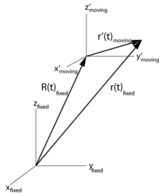
Figure 12.2.1:Inertial reference frame (unprimed), and translational accelerating frame (primed).

Consider an inertial system $(x_{fix},y_{fix},z_{fix})$ which is fixed in space, and a non-inertial system $(x^{\prime}_{mov}, y^{\prime}_{mov}, z^{\prime}_{mov})$ that is moving in a direction relative to the fixed frame such as to maintain constant orientations of the axes relative to the fixed frame, as illustrated in Figure 12.2.1. The fixed frame is designated to be the unprimed frame and, to avoid confusion the subscript $fix$ is attached to the fixed coordinates taken with respect to the fixed coordinate frame. Similarly, the translating reference frame, which is undergoing translational acceleration, has the subscript $mov$ attached to the coordinates taken with respect to the translating frame of reference. Newton’s Laws of motion are obeyed only in the inertial (unprimed) reference frame. The respective position vectors are related by

\mathbf{r}_{fix} = \mathbf{R}_{fix}+\mathbf{r}^{\prime}_{mov} \tag{12.1}

where $\mathbf{r}_{fix}$ is the vector relative to the fixed frame, $\mathbf{r}^{\prime}_{mov}$ is the vector relative to the translationally accelerating frame and $\mathbf{R}_{fix}$ is the vector from the origin of the fixed frame to the origin of the accelerating frame. Differentiating Equation 12.1 gives the velocity vector relation

\mathbf{v}_{fix} = \mathbf{V}_{fix}+ \mathbf{v}^{\prime}_{mov} \tag{12.2}

where $\mathbf{v}_{fix} = \frac{d\mathbf{r}_{fix}}{dt}$ , $\mathbf{v}^{\prime}_{mov} = \frac{d\mathbf{r}^{\prime}_{mov}}{dt}$ and $\mathbf{V}_{fix} = \frac{d\mathbf{R}_{fix}}{dt}$ . Similarly the acceleration vector relation is

\mathbf{a}_{fix} = \mathbf{A}_{fix}+ \mathbf{a}^{\prime}_{mov} \tag{12.3}

where $\mathbf{a}_{fix} = \frac{d^2\mathbf{r}_{fix}}{dt^2}$ , $\mathbf{a}^{\prime}_{mov} = \frac{d^2\mathbf{r}^{\prime}_{mov}}{dt^2}$ and $\mathbf{A}_{fix} = \frac{d^2\mathbf{R}_{fix}}{dt^2}$ .

In the fixed frame, Newton’s laws give that

\mathbf{F}_{fix} = m\mathbf{a}_{fix} \tag{12.4}

The force in the fixed frame can be separated into two terms, the acceleration of the accelerating frame of reference $\mathbf{A}_{fix}$ plus the acceleration with respect to the accelerating frame $\mathbf{a}^{\prime}_{mov}$ .

\mathbf{F}_{fix} = m\mathbf{A}_{fix}+ m\mathbf{a}^{\prime}_{mov} \tag{12.5}

Relative to the accelerating reference frame the acceleration is given by

m\mathbf{a}^{\prime}_{mov} = \mathbf{F}_{fix} - m\mathbf{A}_{fix} \tag{12.6}

The accelerating frame of reference can exploit Newton’s Laws of motion using an effective translational force $\mathbf{F}^{\prime}_{tran} \equiv \mathbf{F}_{fix} − m\mathbf{A}_{fix}$ . The additional $-m\mathbf{A}_{fix}$ term is called an inertial force; it can be altered by choosing a different non-inertial frame of reference, that is, it is dependent on the frame of reference in which the observer is situated.

12.3: Rotating Reference Frame¶

Consider a rotating frame of reference which will be designated as the double-primed (rotating) frame to differentiate it from the non-rotating primed (moving) frame, since both of which may be undergoing translational acceleration relative to the inertial fixed unprimed frame as described in Figure 12.2.1.

Spatial time derivatives in a rotating, non-translating, reference frame¶

For simplicity assume that $\mathbf{R}_{fix} = \mathbf{V}_{fix} = 0$ , that is, the primed reference frame is stationary and identical to the fixed stationary unprimed frame. The double-primed (rotating) frame is a non-inertial frame rotating with respect to the origin of the fixed primed frame.

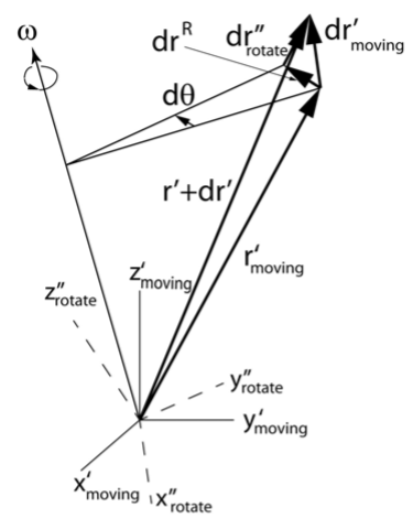
Figure 12.3.1:Infinitessimal displacement in the non rotating primed frame and in the rotating double-primed reference frame.

Appendix $19.4.2C$ shows that an infinitessimal rotation $d\theta$ about an instantaneous axis of rotation leads to an infinitessimal displacement $d\mathbf{r}^{R}$ where

d\mathbf{r}^{R} = d \theta \times \mathbf{r}^{\prime}_{mov} \tag{12.7}

Consider that during a time $dt$ , the position vector in the fixed primed reference frame moves by an arbitrary infinitessimal distance $d\mathbf{r}^{\prime}_{mov}$ . As illustrated in Figure 12.3.1, this infinitessimal distance in the primed non-rotating frame can be split into two parts:

$d\mathbf{r}^{R} = d\theta \times \mathbf{r}^{\prime}_{mov}$ which is due to rotation of the rotating frame with respect to the translating primed frame.
$(d\mathbf{r}^{\prime\prime}_{rot})$ which is the motion with respect to the rotating (double-primed) frame.

That is, the motion has been arbitrarily divided into a part that is due to the rotation of the double-primed frame, plus the vector displacement measured in this rotating (double-primed) frame. It is always possible to make such a decomposition of the displacement as long as the vector sum can be written as

d\mathbf{r}^{\prime}_{mov} = d\mathbf{r}^{\prime\prime}_{rot} + d\theta \times \mathbf{r}^{\prime}_{mov} \tag{12.8}

Since $d\theta = \omega dt$ then the time differential of the displacement, Equation 12.8, can be written as

\left( \frac{d\mathbf{r}^{\prime}}{dt}\right)_{mov} = \left(\frac{d\mathbf{r}^{\prime\prime}}{dt}\right)_{rot} + \omega \times \mathbf{r}^{\prime}_{mov} \tag{12.9}

The important conclusion is that a velocity measured in a non-rotating reference frame $\left(\frac{d\mathbf{r}^{\prime}}{dt}\right)_{mov}$ can be expressed as the sum of the velocity $\left(\frac{d\mathbf{r}^{\prime\prime}}{dt}\right)_{rot}$ , measured relative to a rotating frame, plus the term $\omega \times \mathbf{r}^{\prime}_{mov}$ which accounts for the rotation of the frame. The division of the $d\mathbf{r}^{\prime}_{rot}$ vector into two parts, a part due to rotation of the frame plus a part with respect to the rotating frame, is valid for any vector as shown below.

General vector in a rotating, non-translating, reference frame¶

Consider an arbitrary vector $\mathbf{G}$ which can be expressed in terms of components along the three unit vector basis $\hat{\mathbf{e}}^{fix}_i$ in the fixed inertial frame as

\mathbf{G} = \sum^{3}_{i=1} G^{fix}_i \hat{\mathbf{e}}_i^{fix} \tag{12.10}

Neglecting translational motion, then it can be expressed in terms of the three unit vectors in the non-inertial rotating frame unit vector basis $\hat{\mathbf{e}}^{rot}_i$ as

\mathbf{G} = \sum^{3}_{i=1} (G_i)_{rot} \hat{\mathbf{e}}^{rot}_i \tag{12.11}

Since the unit basis vectors $\hat{\mathbf{e}}^{rot}_i$ are constant in the rotating frame, that is,

\left(\frac{d\hat{\mathbf{e}}^{rot}_i}{dt}\right)_{rot} = 0 \tag{12.12}

then the time derivatives of $\mathbf{G}$ in the rotating coordinate system $\hat{\mathbf{e}}^{rot}_i$ can be written as

\left(\frac{d\mathbf{G}}{dt}\right)_{rot} = \sum^3_{i-1} \left(\frac{dG_i}{dt}\right)_{rot} \hat{\mathbf{e}}^{rot}_i \tag{12.13}

The inertial-frame time derivative taken with components along the rotating coordinate basis $\hat{\mathbf{e}}^{rot}_i$ , Equation 12.11, is

\left(\frac{d\mathbf{G}}{dt}\right)_{fix} = \sum^3_{i-1} \left(\frac{dG_i}{dt}\right)_{rot} \hat{\mathbf{e}}^{rot}_i + (G_i)_{rot} \frac{d\hat{\mathbf{e}}^{rot}_i }{dt} \tag{12.14}

Substitute the unit vector $\hat{\mathbf{e}}^{rot}$ for $\mathbf{r}^{\prime}_{mov}$ in Equation 12.9, plus using Equation 12.12, gives that

\left(\frac{d\hat{\mathbf{e}}^{rot}}{dt}\right)_{fix} = \omega \times \hat{\mathbf{e}}^{rot} \tag{12.15}

Substitute this into the second term of Equation 12.14 gives

\left(\frac{d\mathbf{G}}{dt}\right)_{fix} = \left(\frac{d\mathbf{G}}{dt}\right)_{rot} + \omega \times \mathbf{G} \tag{12.16}

This important identity relates the time derivatives of any vector expressed in both the inertial frame and the rotating non-inertial frame bases. Note that the $\omega \times \mathbf{G}$ term originates from the fact that the unit basis vectors of the rotating reference frame are time dependent with respect to the non-rotating frame basis vectors as given by Equation 12.15. Equation 12.16 is used extensively for problems involving rotating frames. For example, for the special case where $\mathbf{G} = \mathbf{r}^{\prime}$ , then Equation 12.16 relates the velocity vectors in the fixed and rotating frames as given in Equation 12.9.

Another example is the vector $\mathbf{\dot{\omega}}$

\mathbf{\dot{\omega}} = \left(\frac{d\omega}{dt}\right)_{fix} = \left(\frac{d\omega}{dt}\right)_{rot} + \omega \times \omega = \left(\frac{d\omega}{dt}\right)_{rot} = \mathbf{\dot{\omega}} \tag{12.17}

That is, the angular acceleration $\dot{\omega}$ has the same value in both the fixed and rotating frames of reference.

12.4: Reference Frame Undergoing Rotation Plus Translation¶

Consider the case where the system is accelerating in translation as well as rotating, that is, the primed frame is the non-rotating translating frame. The position vector $\mathbf{r}_{fix}$ is taken with respect to the inertial fixed unprimed frame which can be written in terms of the fixed unit basis vectors $(\widehat{\mathbf{i}}_{fix}, \widehat{\mathbf{j}}_{fix}, \widehat{\mathbf{k}}_{fix})$ . This $\mathbf{r}_{fix}$ vector can be written as the vector sum of the translational motion $\mathbf{R}_{fix}$ of the origin of the rotating system with respect to the fixed frame, plus the position $\mathbf{r}^{\prime}_{mov}$ with respect to this translating primed frame basis

\mathbf{r}_{fix} = \mathbf{R}_{fix} + \mathbf{r}^{\prime}_{mov} \tag{12.18}

The time differential is

\left(\frac{d\mathbf{r}}{dt}\right)_{fix} = \left(\frac{d\mathbf{R}}{dt}\right)_{fix} + \left(\frac{d\mathbf{r}^{\prime}_{mov}}{dt}\right) \tag{12.19}

The vector $d\mathbf{r}^{\prime}$ is the position with respect to the translating frame of reference which can be expressed in terms of the unit vectors $\left(\widehat{\mathbf{i}^{\prime}}_{mov}, \widehat{\mathbf{j}^{\prime}}_{mov}, \widehat{\mathbf{k}^{\prime}}_{mov}\right)$ .

Equation 12.19 takes into account the translational motion of the moving primed frame basis. Now, assuming that the double primed frame rotates about the origin of the moving primed frame, then the net displacement with respect to the original inertial frame basis can be combined with equation $(12.3.3)$ leading to the relation

\left(\frac{d\mathbf{r}}{dt}\right)_{fix} = \left(\frac{d\mathbf{R}}{dt}\right)_{fix} + \left(\frac{d\mathbf{r}^{\prime\prime}}{dt}\right)_{rot} + \omega \times \mathbf{r}^{\prime}_{mov} \tag{12.20}

Here the double-primed frame is both rotating and translating. Vectors in this frame are expressed in terms of the unit basis vectors $\left(\widehat{\mathbf{i}^{\prime\prime}}_{rot}, \widehat{\mathbf{j}^{\prime\prime}}_{rot}, \widehat{\mathbf{k}^{\prime\prime}}_{rot}\right)$ .

Expressed as velocities, Equation 12.20 can be written as

\mathbf{v}_{fix} = \mathbf{V}_{fix} + \mathbf{v}^{\prime\prime}_{rot} + \omega \times \mathbf{r}^{\prime}_{mov} \tag{12.21}

where:

$\mathbf{v}_{fix}$ is the velocity measured with respect to the inertial (unprimed) frame basis.
$\mathbf{V}_{fix}$ is the velocity of the origin of the non-inertial translating (primed) frame basis with respect to the origin of the inertial (unprimed) frame basis.
$\mathbf{v}^{\prime\prime}_{rot}$ is the velocity of the particle with respect to the non-inertial rotating (double-primed) frame basis the origin of which is both translating and rotating.
$\omega \times \mathbf{r}^{\prime}_{mov}$ is the motion of the rotating (double-primed) frame with respect to the linearly-translating (primed) frame basis. Thus this relation takes into account both the translational velocity plus rotation of the reference coordinate frame basis vectors.

12.5: Newton’s Law of Motion in a Non-Inertial Frame¶

The acceleration of the system in the rotating inertial frame can be derived by differentiating the general velocity relation for $\mathbf{v}$ , Equation 12.4.4, in the fixed frame basis which gives

\begin{align} \mathbf{a}_{fix} &= \left(\frac{d\mathbf{v}_{fix}}{dt}\right)_{fixed} \\[4pt] &= \left(\frac{d\mathbf{V}_{fix}}{dt}\right)_{fixed} + \left(\frac{d\mathbf{v}^{\prime\prime}_{rot}}{dt}\right)_{fixed} + \left(\frac{d\omega}{dt}\right)_{fixed} \times \mathbf{r}^{\prime}_{mov} + \omega \times \left(\frac{d\mathbf{r}^{\prime}_{mov}}{dt}\right)_{fixed} \tag{12.22} \end{align}

Now we wish to use the general transformation to a rotating frame basis which requires inclusion of the time dependence of the unit vectors in the rotating frame, that is,

\begin{align} \left(\frac{d\mathbf{v}^{\prime\prime}_{rot}}{dt}\right)_{fixed} &= \left(\frac{d\mathbf{v}^{\prime\prime}_{rot}}{dt}\right)_{rotating} + \omega \times \mathbf{v}^{\prime\prime}_{rot} \tag{12.23} \\[4pt] \left(\frac{d\omega}{dt}\right)_{fixed} \times \mathbf{r}^{\prime}_{mov} &= \left(\frac{d\omega}{dt}\right)_{rot} \times \mathbf{r}^{\prime}_{mov} \tag{12.24} \\[4pt] \omega \times \left(\frac{d\mathbf{r}^{\prime}_{mov}}{dt}\right)_{fixed} &= \omega \times \mathbf{v}^{\prime\prime}_{rot} + \omega \times (\omega \times \mathbf{r}^{\prime}_{mov}) \tag{12.25} \end{align}

Using Equations 12.23, 12.24, 12.25 gives

\mathbf{a}_{fix} = \mathbf{A}_{fix} + \mathbf{a}^{\prime\prime}_{rot} + 2\omega \times \mathbf{v}^{\prime\prime}_{rot} + \omega \times (\omega \times \mathbf{r}^{\prime}_{mov}) + \dot{\omega} \times \mathbf{r}^{\prime}_{mov} \tag{12.26}

where the acceleration in the rotating frame is $\mathbf{a}^{\prime\prime}_{rot} = \left(\frac{d\mathbf{v}^{\prime\prime}_{rot}}{dt}\right)_{rot}$ while the velocity is $\mathbf{v}^{\prime\prime}_{rot} = \left(\frac{\mathbf{r}^{\prime\prime}_{rot}}{dt}\right)_{rot}$ and $\mathbf{A}_{fix}$ is with respect to the fixed frame.

Newton’s laws of motion are obeyed in the inertial frame, that is

\begin{align} \mathbf{F}_{fix} &= m\mathbf{a}_{fix} \\[4pt] &= m(\mathbf{A}_{fix} + \mathbf{a}^{\prime\prime}_{rot} + 2\omega \times \mathbf{v}^{\prime\prime}_{rot} + \omega \times (\omega \times \mathbf{r}^{\prime}_{mov}) + \dot{\omega} \times \mathbf{r}^{\prime}_{mov}) \tag{12.27} \end{align}

In the double-primed frame, which may be both rotating and accelerating in translation, one can ascribe an effective force $\mathbf{F}^{eff}_{rot}$ that obeys an effective Newton’s law for the acceleration $\mathbf{a}^{\prime\prime}_{rot}$ in the rotating frame

\begin{align}\mathbf{F}^{eff}_{rot} &= m\mathbf{a}^{\prime\prime}_{rot} \\[4pt] &= \mathbf{F}_{fix} - m(\mathbf{A}_{fix} + 2\omega \times \mathbf{v}^{\prime\prime}_{rot} + \omega \times (\omega \times \mathbf{r}^{\prime}_{mov}) + \dot{\omega} \times \mathbf{r}^{\prime}_{mov}) \tag{12.28} \end{align}

Note that the effective force $\mathbf{F}^{eff}_{rot}$ comprises the physical force $\mathbf{F}_{fixed}$ minus four non-inertial forces that are introduced to correct for the fact that the rotating reference frame is a non-inertial frame.

12.6: Lagrangian Mechanics in a Non-Inertial Frame¶

The above derivation of the equations of motion in the rotating frame is based on Newtonian mechanics. Lagrangian mechanics provides another derivation of these equations of motion for a rotating frame of reference by exploiting the fact that the Lagrangian is a scalar which is frame independent, that is, it is invariant to rotation of the frame of reference.

The Lagrangian in any frame is given by

L = \frac{1}{2} m \mathbf{v} \cdot \mathbf{v} - U(r) \tag{12.29}

The scalar product $\mathbf{v} \cdot \mathbf{v}$ is the same in any rotated frame and can be evaluated in terms of the rotating frame variables using the same decomposition of the translational plus rotational motion as used previously and given in equation $(12.4.4)$ .

Equation $(12.4.4)$ decomposes the velocity in the fixed inertial frame $\mathbf{v}_{fix}$ into four vector terms, the translational velocity $\mathbf{V}_{fix}$ of the translating frame, the velocity in the rotating-translating frame $\mathbf{v}^{\prime\prime}_{rot}$ , and rotational velocity $(\omega \times \mathbf{r}^{\prime}_{mov})$ . Using equations 12.29 and $(12.4.4)$ , plus appendix equation 19.2.21 for the triple products, gives that the Lagrangian evaluated using $\mathbf{v}_{fix}\cdot \mathbf{v}_{fix}$ equals

L = \frac{1}{2} m \left[ \mathbf{V}_{fix}\cdot \mathbf{V}_{fix} + \mathbf{v}^{\prime\prime}_{rot} \cdot \mathbf{v}^{\prime\prime}_{rot} + 2\mathbf{V}_{fix} \cdot \mathbf{v}^{\prime\prime}_{rot} + 2\mathbf{V}_{fix} \cdot (\omega \times \mathbf{r}^{\prime}_{mov})+2\mathbf{v}^{\prime\prime}_{rot} \cdot (\omega \times \mathbf{r}^{\prime}_{mov})+(\omega \times \mathbf{r}^{\prime}_{mov})^2 \right] −U(r) \tag{12.30}

This can be used to derive the canonical momentum in the rotating frame

\mathbf{p}^{\prime\prime}_{rot} = \frac{\partial L}{\partial \mathbf{v}^{\prime\prime}_{rot}} = m [\mathbf{V}_{fix}+\mathbf{v}^{\prime\prime}_{rot} + \omega \times \mathbf{r}^{\prime}_{mov}] \tag{12.31}

The Lagrange equations can be used to derive the equations of motion in terms of the variables evaluated in the rotating reference frame. The required Lagrange derivatives are

\frac{d}{dr}\frac{\partial L}{\partial \mathbf{v}^{\prime\prime}_{rot}} = m [\mathbf{A}_{fix}+\mathbf{a}^{\prime\prime}_{rot} + (\omega \times \mathbf{v}^{\prime\prime}_{rot})+(\dot{\omega} \times \mathbf{r}^{\prime}_{mov})]_{rot} \tag{12.32}

and

\frac{\partial L}{ \partial \mathbf{r}^{\prime}} = −m [(\omega \times \mathbf{V}_{fix}) − (\omega \times \mathbf{v}^{\prime\prime}_{rot}) − \omega \times (\omega \times \mathbf{r}^{\prime}_{mov})]_{rot} − \nabla U \tag{12.33}

where the scalar triple product, equation 19.2.21, has been used. Thus the Lagrange equations give for the rotating frame basis that

m\mathbf{a}^{\prime\prime}_{rot} = −\nabla U − m[\mathbf{A}_{fix}+ (\omega \times\mathbf{V}_{fix}) +2 (\omega \times \mathbf{v}^{\prime\prime}_{rot}) + \omega \times (\omega \times \mathbf{r}^{\prime}_{mov})+(\dot{\omega} \times \mathbf{r}^{\prime}_{mov})]_{rot} \tag{12.34}

The external force is identified as $\mathbf{F}_{fixed} = −\nabla U$ . Equation $(12.3.7)$ can be used to transform between the fixed and the rotating bases.

\mathbf{A}_{fix} = \left[ \mathbf{A}_{fix} + (\omega \times \mathbf{V})_{fix}\right]_{rot} \tag{12.35}

This leads to an effective force in the non-inertial translating plus rotating frame that corresponds to an effective Newtonian force of

\mathbf{F}^{eff}_{rot} = m\mathbf{a}^{\prime\prime}_{rot} = \mathbf{F} − m[\mathbf{A}_{fix} + 2\omega \times \mathbf{v}^{\prime\prime}_{rot} + \omega \times (\omega \times \mathbf{r}^{\prime}_{mov})+(\dot{\omega} \times \mathbf{r}^{\prime}_{mov})] \tag{12.36}

where $\mathbf{A}_{fix}$ is expressed in the fixed frame. The derivation of Equation 12.36 using Lagrangian mechanics, confirms the identical formula 12.29 derived using Newtonian mechanics.

The four correction terms for the non-inertial frame basis correspond to the following effective forces.

Translational acceleration: $\mathbf{F}^{eff}_{mov} = −m\mathbf{A}_{fix}$ is the usual inertial force experienced in a linearly accelerating frame of reference, and where $\mathbf{A}_{fix}$ is with respect to the fixed frame.
Coriolis force: $\mathbf{F}^{eff}_{cor} = −2m\omega \times \mathbf{v}^{\prime\prime}_{rot}$ This is a new type of inertial force that is present only when a particle is moving in the rotating frame. This force is proportional to the velocity in the rotating frame and is independent of the position in the rotating frame
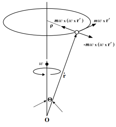
Centrifugal force: $\mathbf{F}^{eff}_{ef} = −m\omega \times (\omega \times \mathbf{r}^{\prime}_{mov})$ This is due to the centripetal acceleration of the particle owing to the rotation of the moving axis about the axis of rotation.
Transverse (azimuthal) force: $\mathbf{F}^{eff}_{az} = −m\dot{\omega} \times \mathbf{r}^{\prime}_{mov}$ This is a straightforward term due to acceleration of the particle due to the angular acceleration of the rotating axes.

The above inertial forces are correction terms arising from trying to extend Newton’s laws of motion to a non-inertial frame involving both translation and rotation. These correction forces are often referred to as “fictitious” forces. However, these non-inertial forces are very real when located in the non-inertial frame. Since the centrifugal and Coriolis terms are unusual they are discussed below.

12.7: Centrifugal Force¶

The centrifugal force was defined as

\mathbf{F}_{cf} = −m\omega \times (\omega \times \mathbf{r}^{\prime}_{mov}) \tag{12.37}

Note that

\omega \cdot \mathbf{F}_{cf} = 0 \tag{12.38}

therefore the centrifugal force is perpendicular to the axis of rotation. Using the vector identity, equation 19.2.25 allows the centrifugal force to be written as

\mathbf{F}_{cf} = −m [ (\omega \cdot \mathbf{r}^{\prime}_{mov}) \omega − \omega^2\mathbf{r}^{\prime}_{mov}] \tag{12.39}

For the case where the radius $\mathbf{r}^{\prime}$ is perpendicular to $\omega$ then $\omega \cdot \mathbf{r}^{\prime} = 0$ and thus for this special case

\mathbf{F}_{cf} = m\omega^2\mathbf{r}^{\prime}_{mov} \tag{12.40}

The centrifugal force is experienced when riding in a car driven rapidly around a bend. The passenger experiences an apparent centrifugal (center fleeing) force that thrusts them to the outside of the bend relative to the inside of the turning car. In reality, relative to the fixed inertial frame, i.e. the road, the friction between the car tires and the road is changing the direction of the car towards the inside of the bend and the car seat is causing the centripetal (center seeking) acceleration of the passenger. A bucket of water attached to a rope can be swung around in a vertical plane without spilling any water if the centrifugal force exceeds the gravitation force at the top of the trajectory.

12.8: Coriolis Force¶

The Coriolis force was defined to be

\mathbf{F}_{cor} = -2m\omega \times \mathbf{v}^{\prime\prime}_{rot} \tag{12.41}

where $\mathbf{v}^{\prime\prime}$ is the velocity measured in the rotating (double-primed) frame. The Coriolis force is an interesting force; it is perpendicular to both the axis of rotation and the velocity vector in the rotating frame, that is, it is analogous to the $q\mathbf{v} \times \mathbf{B}$ Lorentz magnetic force.

The understanding of the Coriolis effect is facilitated by considering the physics of a hockey puck sliding on a rotating frictionless table. Assume that the table rotates with constant angular frequency $\omega = \omega \widehat{\mathbf{k}}$ about the $z$ axis. For this system the origin of the rotating system is fixed, and the angular frequency is constant, thus $\mathbf{A}$ and $\dot{\omega} \times \mathbf{r}^{\prime}$ are zero. Also it is assumed that there are no external forces acting on the hockey puck, thus the net acceleration of the puck sliding on the table, as seen in the rotating frame, simplifies to

\mathbf{a}^{\prime\prime}_{rot} = -2\omega \times \mathbf{v}^{\prime\prime}_{rot} − \omega \times (\omega \times \mathbf{r}^{\prime}_{mov}) = −2\omega \widehat{\mathbf{k}} \times \mathbf{v}^{\prime\prime}_{rot} + \omega^2\mathbf{r}^{\prime}_{mov} \tag{12.42}

The centrifugal acceleration $+\omega^2\mathbf{r}^{\prime}_{mov}$ is radially outwards while the Coriolis acceleration $−2\omega \widehat{\mathbf{k}} \times \mathbf{v}^{\prime\prime}_{rot}$ is to the right. Integration of the equations of motion can be used to calculate the trajectories in the rotating frame of reference.

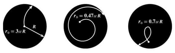
Free-force motion of a hockey puck sliding on a rotating frictionless table of radius R that is rotating with constant angular frequency \omega out of the page. — Figure 12.8.1:Free-force motion of a hockey puck sliding on a rotating frictionless table of radius $R$ that is rotating with constant angular frequency $\omega$ out of the page.

Figure 12.8.1 illustrates trajectories of the hockey puck in the rotating reference frame when no external forces are acting, that is, in the inertial frame the puck moves in a straight line with constant velocity $\mathbf{v}_0$ . In the rotating reference frame the Coriolis force accelerates the puck to the right leading to trajectories that exhibit spiral motion. The apparent complicated trajectories are a result of the observer being in the rotating frame for which that the straight inertial-frame trajectories of the moving puck exhibit a spiralling trajectory in the rotating-frame.

The Coriolis force is the reason that winds circulate in an anticlockwise direction about low-pressure regions in the Earth’s northern hemisphere. It also has important consequences in many activities on earth such as ballet dancing, ice skating, acrobatics, nuclear and molecular rotation, and the motion of missiles.

Example 12.8.1: Accelerating spring plane pendulum

Comparison of the relative merits of using a non-inertial frame versus an inertial frame is given by a spring pendulum attached to an accelerating fulcrum. As shown in the figure, the spring pendulum comprises a mass $m$ attached to a massless spring that has a rest length $r_0$ and spring constant $k$ . The system is in a vertical gravitational field $g$ and the fulcrum of the pendulum is accelerating vertically upwards with a constant acceleration $a$ . Assume that the spring pendulum oscillates only in the vertical $\theta$ plane.

Inertial frame¶

This problem can be solved in the fixed inertial coordinate system with coordinates $(x, y)$ . These coordinates, and their time derivatives, are given in terms of $r$ and $\theta$ by

\begin{align*} x & = r\sin\theta \\[4pt] \dot{x} & = \dot{r}\sin\theta + r\dot{\theta}\cos \theta \\[4pt] y & = -r\cos\theta + \frac{1}{2} a t^2 \\[4pt] \dot{y} &= r \dot{\theta} \sin \theta - \dot{r} \cos\theta + at \end{align*}

Thus

\begin{align*} L &=\frac{1}{2} m\left(\dot{x}^{2}+\dot{y}^{2}\right)-m g y-\frac{1}{2} k\left(r-r_{0}\right)^{2} \\ &=\frac{1}{2} m\left[\dot{r}^{2} + r^{2} \dot{\theta}^{2}+a^{2} t^{2}+2 a t(r \dot{\theta} \sin \theta-\dot{r} \cos \theta)\right] + m g\left(r \cos \theta-\frac{1}{2} a t^{2}\right)-\frac{1}{2} k\left(r-r_{0}\right)^{2} \end{align*}

The Lagrange equations of motion are given by

\begin{align*} \Lambda_{r} L &=0 \\[4pt] \ddot{r}-r \dot{\theta}^{2}-(a+g) \cos \theta+\frac{k}{m}\left(r-r_{0}\right) &=0 \\[4pt] \Lambda_{\theta} L&=0 \\[4pt] \ddot{\theta}+\frac{2}{r} \dot{r} \dot{\theta}+\frac{(a+g)}{r} \sin \theta &=0 \end{align*}

The generalized momenta are

\begin{align*} p_r & = \frac{\partial L}{\partial \dot{r}} \\[4pt] &= m\dot{r} - mat\cos \theta \\ p_{\theta} & = \frac{\partial L}{\partial \dot{\theta}} \\[4pt] &= mr^2 \dot{\theta} + matr \sin \theta \end{align*}

These lead to the corresponding velocities of

\begin{aligned} \dot{r} & = & \frac{p_r}{m} + at \cos \theta \\ \dot{\theta} & = & \frac{p_{\theta}}{mr^2} - \frac{at \sin \theta}{r} \end{aligned}

and thus the Hamiltonian is given by

\begin{align*} H & = p_r \dot{r} + p_{\theta} \dot{\theta} − L \\ & = \frac{p^2_r}{2m} + \frac{p_{\theta}}{2mr^2} - \frac{at}{r} p_{\theta} \sin \theta + atp_r \cos \theta + \frac{1}{2} k (r - r_0)^2 + \frac{1}{2} mgat^2 - mgr \cos \theta \end{align*}

The Hamilton equations of motion give that

\begin{aligned} \dot{r} & = & \frac{\partial H}{\partial p_r} = \frac{p_r}{m} + at \cos \theta \\ \dot{\theta} & = & \frac{\partial H}{\partial p_{\theta}} = \frac{p_{\theta}}{mr^2} − \frac{at \sin \theta}{r} \end{aligned}

These radial and angular velocities are the same as obtained using Lagrangian mechanics. The Hamilton equations for $\dot{p}_r$ and $\dot{p}_\theta$ are given by

\dot{p}_r = −\frac{\partial H}{\partial \theta} = −\frac{at}{r^2} p_{\theta} \sin \theta − k (r − r_0) + mg \cos \theta + \frac{p^2_{\theta}}{mr^3} \nonumber

Similarly

\dot{p}_{\theta} = −\frac{\partial H}{\partial \theta} = \frac{at}{r} p_{\theta} \cos \theta + atp_r \sin \theta − mgr \sin \theta \nonumber

The transformation equations relating the generalized coordinates $r, \theta$ are time dependent so the Hamiltonian $H$ does not equal the total energy $E$ . In addition neither the Lagrangian nor the Hamiltonian are conserved since they both are time dependent. The fact that the Hamiltonian is not conserved is obvious since the whole system is accelerating upwards leading to increasing kinetic and potential energies. Moreover, the time derivative of the angular momentum $\dot{p}_\theta$ is non-zero so the angular momentum $p_{\theta}$ is not conserved.

Non-inertial fulcrum frame¶

This system also can be addressed in the accelerating non-inertial fulcrum frame of reference which is fixed to the fulcrum of the spring of the pendulum. In this non-inertial frame of reference, the acceleration of the frame can be taken into account using an effective acceleration $a$ which is added to the gravitational force; that is, $g$ is replaced by an effective gravitational force $(g + a)$ . Then the Lagrangian in the fulcrum frame simplifies to

L_{fulcrum} = \frac{1}{2} m\dot{r}^2 + r^2 \dot{\theta}^2 + m (g + a) (r \cos \theta ) − \frac{1}{2} k (r − r_0)^2 \nonumber

The Lagrange equations of motion in the fulcrum frame are given by

\begin{aligned} \Lambda_{r} L_{fulcrum}=0 && \\ && \ddot{r}-r \dot{\theta}^{2}-(a+g) \cos \theta+\frac{k}{m}\left(r-r_{0}\right)=0 \end{aligned}

\begin{aligned} \Lambda_{\theta} L_{fulcrum}=0 && \\ && \ddot{\theta}+\frac{2}{r} \dot{r} \dot{\theta}+\frac{(a+g)}{r} \sin \theta=0 \end{aligned}

These are identical to the Lagrange equations of motion derived in the inertial frame.

The $L_{fulcrum}$ can be used to derive the momenta in the non-inertial fulcrum frame

\begin{aligned} \tilde{p}_r & = & \frac{\partial L_{fulcrum}}{\partial \dot{r}} = m\dot{r} \\ \tilde{p}_{\theta} & = & \frac{\partial L_{fulcrumr}}{\partial \dot{\theta}} = mr^2 \dot{\theta} \end{aligned}

which comprise only a part of the momenta derived in the inertial frame. These partial fulcrum momenta lead to a Hamiltonian for the fulcum-frame of

H_{fulcrum}=\tilde{p}_{r} \dot{r}+\tilde{p}_{\theta} \dot{\theta}-L_{fulcrum}=\frac{\tilde{p}_{r}^{2}}{2 m}+\frac{\tilde{p}_{\theta}}{2 m r^{2}}+\frac{1}{2} k\left(r-r_{0}\right)^{2}-m(g+a) r \cos \theta \nonumber

Both $L_{fulcrum}$ and $H_{fulcrum}$ are time independent and thus the fulcrum Hamiltonian $H_{fulcrum}$ is a constant of motion in the fulcrum frame. However, $H_{fulcrum}$ does not equal the total energy which is increasing with time due to the acceleration of the fulcrum frame relative to the inertial frame. This example illustrates that use of non-inertial frames can simplify solution of accelerating systems.

Example 12.8.2: Surface of rotating liquid

Find the shape of the surface of liquid in a bucket that rotates with angular speed $\omega$ as shown in the adjacent figure. Assume that the liquid is at rest in the frame of the bucket. Therefore, in the coordinate system rotating with the bucket of liquid, the centrifugal force is important whereas the Coriolis, translational, and transverse forces are zero. The external force

\mathbf{F} = \mathbf{F}^{\prime} − m\mathbf{g} \nonumber

where $\mathbf{F}^{\prime}$ is the pressure which is perpendicular to the surface. At equilibrium the acceleration of the surface is zero that is

m\mathbf{a}^{\prime\prime} =0= \mathbf{F}^{\prime} + m (\mathbf{g} − \omega \times (\omega \times \mathbf{r}^{\prime} )) \nonumber

The effective gravitational force is

\mathbf{g}_{eff} = (\mathbf{g} − \omega \times (\omega \times \mathbf{r}^{\prime} )) \nonumber

which must be perpendicular to the surface of the liquid since $\mathbf{F}^{\prime}$ is perpendicular to the surface of a fluid, and the net force is zero. In cylindrical coordinates this can be written as

\mathbf{g}_{eff} = −g\widehat{\mathbf{z}} + \rho \omega^2 \widehat{\mathbf{p}} \nonumber

From the figure it can be deduced that

\tan \theta = \frac{dz}{d\rho} = \frac{\rho \omega^2}{g}\nonumber

By integration

z = \frac{\omega^2}{2g} \rho^2 + \text{ constant} \nonumber

This is the equation of a paraboloid and corresponds to a parabolic gravitational equipotential energy surface. Astrophysicists build large parabolic mirrors for telescopes by continuously spinning a large vat of glass while it solidifies. This is much easier than grinding a large cylindrical block of glass into a parabolic shape.

Example 12.8.3: The pirouette

An interesting application of the Coriolis force is the problem of a spinning ice skater or ballet dancer. Her angular frequency increases when she draws in her arms. The conventional explanation is that angular momentum is conserved in the absence of any external forces which is correct. Thus since her moment of inertia decreases when she retracts her arms, her angular velocity must increase to maintain a constant angular momentum $\mathbf{L} = I \omega$ . But this explanation does not address the question as to what are the forces that cause the angular frequency to increase? The real radial forces the skater feels when she retracts her arms cannot directly lead to angular acceleration since radial forces are perpendicular to the rotation. The following derivation shows that the Coriolis force $−2m\omega \times \mathbf{v}^{\prime\prime}_{rot}$ acts tangentially to the radial retraction velocity of her arms leading to the angular acceleration required to maintain constant angular momentum.

Consider that a mass $m$ is moving radially at a velocity $\dot{r}^{\prime\prime}_{rot}$ then the Coriolis force in the rotating frame is

\mathbf{F}_{cor} = −2m\omega \times \mathbf{\dot{r}}^{\prime\prime}_{rot} \nonumber

This Coriolis force leads to an angular acceleration of the mass of

\dot{\omega} = -\frac{2\omega \times \mathbf{\dot{r}}^{\prime\prime}_{rot}}{r^{\prime\prime}} \tag{$\alpha$}

that is, the rotational frequency decreases if the radius is increased. Note that, as shown in equation $(12.3.11)$ , $\dot{\omega} = \dot{\omega}^{\prime\prime}$ . This nonzero value of $\dot{\omega}$ obviously leads to an azimuthal force in addition to the Coriolis force. Consider the rate of change of angular momentum for the rotating mass $m$ assuming that the angular momentum comes purely from the rotation $\omega$ . Then in the rotating frame

\mathbf{\dot{p}}_{\theta^{\prime\prime}} = \frac{d}{dt} (m r^{\prime\prime 2} \omega ) = 2mr^{\prime\prime} \dot{r}^{\prime\prime} \omega + mr^{\prime\prime 2} \mathbf{\dot{\omega}} \nonumber

Substituting Equation alpha for $\dot{\omega}$ in the second term gives

\mathbf{\dot{p}}_{\theta ''} = 2mr^{\prime\prime} \dot{r}^{\prime\prime} \omega - 2mr^{\prime\prime} \dot{r}^{\prime\prime} \omega = 0 \nonumber

That is, the two terms cancel. Thus the angular momentum is conserved for this case where the velocity is radial. Note that, since ${p_{\theta}}^{''}$ is assumed to be colinear with $\omega$ , then it is the same in both the stationary and rotating frames of reference and thus angular momentum is conserved in both frames. In addition, in the fixed frame, the angular momentum is conserved if no external torques are acting as assumed above.

Note that the rotational energy is

E_{rot} = \frac{1}{2} I \omega^2 \nonumber

Also the angular momentum is conserved, that is

\mathbf{p}_{\theta} = I\omega = I \hat{\omega} \nonumber

Substituting $\omega = \frac{p_{\theta}}{I}$ in the rotational energy gives

E_{rot} = \frac{p^{2}_{\theta}}{2I} = \frac{l^2}{2I} \nonumber

Therefore the rotational energy actually increases as the moment of inertia decreases when the ice skater pulls her arms close to her body. This increase in rotational energy is provided by the work done as the dancer pulls her arms inward against the centrifugal force.

12.9: Routhian Reduction for Rotating Systems¶

The Routhian reduction technique, that was introduced in chapter 8.6, is a hybrid variational approach. It was devised by Routh to handle the cyclic and non-cyclic variables separately in order to simultaneously exploit the differing advantages of the Hamiltonian and Lagrangian formulations. The Routhian reduction technique is a powerful method for handling rotating systems ranging from galaxies to molecules, or deformed nuclei, as well as rotating machinery in engineering. A valuable feature of the Hamiltonian formulation is that it allows elimination of cyclic variables which reduces the number of degrees of freedom to be handled. As a consequence, cyclic variables are called ignorable variables in Hamiltonian mechanics. The Lagrangian, the Hamiltonian and the Routhian all are scalars under rotation and thus are invariant to rotation of the frame of reference. Note that often there are only two cyclic variables for a rotating system, that is, $\dot{\theta} = \boldsymbol{\omega}$ and the corresponding canonical total angular momentum $p_{\theta} = \mathbf{J}$ .

As mentioned in chapter 8.6, there are two possible Routhians that are useful for handling rotation frames of reference. For rotating systems the cyclic Routhian $R_{cyclic}$ simplifies to

R_{cyclic}\left(q_{1}, \ldots, q_{n} ; \dot{q}_{1}, \ldots, \dot{q}_{s} ; p_{s+1}, \ldots, p_{n} ; t\right)=H_{cyclic}-L_{noncyclic}=\boldsymbol{\omega} \cdot \mathbf{J}-L \tag{12.43}

This Routhian behaves like a Hamiltonian for the ignorable cyclic coordinates $\omega, \mathbf{J}$ . Simultaneously it behaves like a negative Lagrangian $L_{noncyclic}$ for all the other coordinates.

The non-cyclic Routhian $R_{noncyclic}$ complements $R_{cyclic}$ in that it is defined as

R_{noncyclic}\left(q_{1}, \ldots, q_{n} ; p_{1}, \ldots, p_{s} ; \dot{q}_{s+1}, \ldots, \dot{q}_{n} ; t\right)=H_{noncyclic}-L_{cyclic}=H - \boldsymbol{\omega} \cdot \mathbf{J} \tag{12.44}

This non-cyclic Routhian behaves like a Hamiltonian for all the non-cyclic variables and behaves like a negative Lagrangian for the two cyclic variables $\omega , p_{\omega}$ . Since the cyclic variables are constants of motion, then $R_{noncyclic}$ is a constant of motion that equals the energy in the rotating frame if $H$ is a constant of motion. However, $R_{noncyclic}$ does not equal the total energy since the coordinate transformation is time dependent, that is, the Routhian $R_{noncyclic}$ corresponds to the energy of the non-cyclic parts of the motion.

For example, the Routhian $R_{noncyclic}$ for a system that is being cranked about the $\phi$ axis at some fixed angular frequency $\dot{\phi} = \omega$ , with corresponding total angular momentum $\mathbf{p}\phi = \mathbf{J}$ , can be written as^[1]

\begin{align} R_{noncyclic} & = & H − \boldsymbol{\omega} \cdot \mathbf{J} \tag{12.45} \\ & = & \frac{1}{2} m \left[ \mathbf{V} \cdot \mathbf{V} + \mathbf{v}^{\prime\prime} \cdot \mathbf{v}^{\prime\prime}+2\mathbf{V} \cdot \mathbf{v}^{\prime\prime}+2\mathbf{V} \cdot (\boldsymbol{\omega} \times \mathbf{r}^{\prime} )+2v^{\prime\prime} \cdot (\boldsymbol{\omega} \times \mathbf{r}^{\prime} )+(\boldsymbol{\omega} \times \mathbf{r}^{\prime} )^2 \right] − \boldsymbol{\omega} \cdot \mathbf{J} + U(r) \notag \end{align}

Note that $R_{noncyclic}$ is a constant of motion if $\frac{\partial L}{\partial t} = 0$ , which is the case when the system is being cranked at a constant angular frequency. However the Hamiltonian in the rotating frame $H_{rot} = H − \boldsymbol{\omega} \cdot \mathbf{J}$ is given by $R_{noncyclic} = H_{rot} \neq E$ since the coordinate transformation is time dependent. The canonical Hamilton equations for the fourth and fifth terms in the bracket can be identified with the Coriolis force $2m\boldsymbol{\omega} \times \mathbf{v}^{\prime\prime}$ , while the last term in the bracket is identified with the centrifugal force. That is, define

U_{cf} \equiv - \frac{1}{2} m (\boldsymbol{\omega} \times \mathbf{r}^{\prime} )^2 \tag{12.46}

where the gradient of $U_{cf}$ gives the usual centrifugal force.

\mathbf{F}_{c f}=-\nabla U_{c f}=\frac{m}{2} \nabla\left[\omega^{2} r^{\prime 2}-\left(\boldsymbol{\omega} \cdot \mathbf{r}^{\prime}\right)^{2}\right]=m\left[\omega^{2} \mathbf{r}^{\prime}-\left(\boldsymbol{\omega} \cdot \mathbf{r}^{\prime}\right) \boldsymbol{\omega}\right]=-m \boldsymbol{\omega} \times\left(\boldsymbol{\omega} \times \mathbf{r}^{\prime}\right)\tag{12.47}

The Routhian reduction method is used extensively in science and engineering to describe rotational motion of rigid bodies, molecules, deformed nuclei, and astrophysical objects. The cyclic variables describe the rotation of the frame and thus the Routhian $R_{noncyclic} = H_{rot}$ corresponds to the Hamiltonian for the non-cyclic variables in the rotating frame.

Example 12.9.1: Cranked plane pendulum

$Cranked plane pendulum that is cranked around the vertical axis with angular velocity \dot{\phi} = \omega.$

Figure 12.9.1:Cranked plane pendulum that is cranked around the vertical axis with angular velocity $\dot{\phi} = \omega$ .

The cranked plane pendulum, which is also called the rotating plane pendulum, comprises a plane pendulum that is cranked around a vertical axis at a constant angular velocity $\dot{\phi} = \omega$ as determined by some external drive mechanism. The parameters are illustrated in the adjacent figure. The cranked pendulum nicely illustrates the advantages of working in a non-inertial rotating frame for a driven rotating system. Although the cranked plane pendulum looks similar to the spherical pendulum, there is one very important difference; for the spherical pendulum $p_{\phi} = ml^2 \sin^2 \theta \dot{\phi}$ is a constant of motion and thus the angular velocity varies with $\theta$ , i.e. $\dot{\phi} = \frac{p_{\phi}}{ml^2 \sin^2 \theta}$ , whereas for the cranked plane pendulum, the constant of motion is $\dot{\phi} = \omega$ and thus the angular momentum varies with $\theta$ , i.e. $p_{\phi} = l \sin^2 \theta \omega$ . For the cranked plane pendulum, the energy must flow into and out of the cranking drive system that is providing the constraint force to satisfy the equation of constraint

g_{\phi} = \dot{\phi} − \omega = 0 \notag

The easiest way to solve the equations of motion for the cranked plane pendulum is to use generalized coordinates to absorb the equation of constraint and applied constraint torque. This is done by incorporating the $\dot{\phi} = \omega$ constraint explicitly in the Lagrangian or Hamiltonian and solving for just $\theta$ in the rotating frame.

Assuming that $\dot{\phi} = \omega$ , and using generalized coordinates to absorb the cranking constraint forces, then the Lagrangian for the cranked pendulum can be written as.

L = \frac{1}{2} ml^2 (\dot{\theta}^2 + \sin^2 \theta \omega^2) + mgl \cos \theta \notag

The momentum conjugate to $\theta$ is

p_{\theta} = \frac{\partial L}{\partial \dot{\theta}} = ml^2 \dot{\theta} \notag

Consider the Routhian $R_{noncyclic} = p_{\theta} \dot{\theta} − L = H − p_{\phi} \dot{\phi}$ which acts as a Hamiltonian $H_{rot}$ in the rotating frame

R_{noncyclic} = p_{\theta} \dot{\theta} − L = H - p_{\phi} \dot{\phi} = \frac{p^2_{\theta}}{2ml^2} - \frac{1}{2} ml^2 \omega^2 \sin^2 \theta − mgl \cos \theta \nonumber

Note that if $\dot{\phi} = \omega$ is constant, then $R_{noncyclic}$ is a constant of motion for rotation about the $\phi$ axis since it is independent of $\phi$ . Also $\frac{dR_{noncyclic}}{dt} = −\frac{\partial L}{\partial t} = 0$ thus the energy in the rotating non-inertial frame of the pendulum $R_{noncyclic} = H_{rot} = H − p_{\phi} \dot{\phi}$ is a constant of motion, but it does not equal the total energy since the rotating coordinate transformation is time dependent. The driver that cranks the system at a constant $\omega$ provides or absorbs the energy $dW = dE = \omega dp_{\phi}$ as $\theta$ changes in order to maintain a constant $\omega$ .

The Routhian $R_{noncyclic}$ can be used to derive the equations of motion using Hamiltonian mechanics.

\dot{\theta} = \frac{\partial R_{noncyclic}}{\partial p_{\theta}} = \frac{p_{\theta}}{ml^2} \notag

\dot{p}_{\theta} = −\frac{\partial R_{noncyclic}}{\partial \theta} = −mgl \sin \theta \left[ 1 − \frac{l}{g} \cos \theta \omega^2 \right] \nonumber

Since $\dot{p}_{\theta} = m;^2 \ddot{\theta}$ , then the equation of motion is

\ddot{\theta} + \frac{g}{l} \sin \theta \left[ 1 − \frac{l}{g} \cos \theta \omega^2 \right] = 0 \tag{$\alpha$}

Assuming that $\sin \theta \approx \theta$ , then Equation alpha leads to linear harmonic oscillator solutions about a minimum at $\theta = 0$ if the term in brackets is positive. That is, when the bracket $\left[ 1 − \frac{l}{g} \cos \theta \omega^2 \right] > 0$ then equation alpha corresponds to a harmonic oscillator with angular velocity $\Omega$ given by

\Omega^2 = \frac{g}{l} \sin \theta \left[ 1 − \frac{l}{g} \cos \theta \omega^2 \right] \notag

The adjacent figure shows the phase-space diagrams for a plane pendulum rotating about a vertical axis at angular velocity $\omega$ for (a) $\omega < \sqrt{\frac{g}{l}}$ and (b) $\omega > \sqrt{\frac{g}{l}}$ . The upper phase plot shows small $\omega$ when the square bracket of Equation alpha is positive and the phase space trajectories are ellipses around the stable equilibrium point $(0, 0)$ . As $\omega$ increases the bracket becomes smaller and changes sign when $\omega^2 \cos \theta = \frac{g}{l}$ . For larger $\omega$ the bracket is negative leading to hyperbolic phase space trajectories around the $(\theta , p_{\theta} ) = (0, 0)$ equilibrium point, that is, an unstable equilibrium point. However, new stable equilibrium points now occur at angles $(\theta , p_{\theta} ) =(\pm \theta_0, 0)$ where $\cos \theta_0 = \frac{g}{l \omega^2}$ . That is, the equilibrium point $(0, 0)$ undergoes bifurcation as illustrated in the lower figure. These new equilibrium points are stable as illustrated by the elliptical trajectories around these points. It is interesting that these new equilibrium points $\pm \theta_0$ move to larger angles given by $\cos \theta_0 = \frac{g}{l\omega^2}$ beyond the bifurcation point at $\frac{g}{l\omega^2} = 1$ . For low energy the mass oscillates about the minimum at $\theta = \theta_0$ whereas the motion becomes more complicated for higher energy. The bifurcation corresponds to symmetry breaking since, under spatial reflection, the equilibrium point is unchanged at low rotational frequencies but it transforms from $+\theta_0$ to $−\theta_0$ once the solution bifurcates, that is, the symmetry is broken. Also chaos can occur at the separatrix that separates the bifurcation. Note that either the Lagrange multiplier approach, or the generalized force approach, can be used to determine the applied torque required to ensure a constant $\omega$ for the cranked pendulum.

$Phase-space diagrams for the plane pendulum cranked at angular velocity \omega about a vertical axis. [Figure 12.9.2a](#fig-12-9-2) is for \omega < \frac{g}{l} while 12.9.2b is for \omega > \frac{g}{l}.$

Figure 12.9.2:Phase-space diagrams for the plane pendulum cranked at angular velocity $\omega$ about a vertical axis. Figure 12.9.2a is for $\omega < \frac{g}{l}$ while 12.9.2b is for $\omega > \frac{g}{l}$ .

Example 12.9.2: Nucleon orbits in deformed nuclei

Consider the rotation of axially-symmetric, prolate-deformed nucleus. Many nuclei have a prolate spheroidal shape, (the shape of a rugby ball) and they rotate perpendicular to the symmetry axis. In the non-inertial body-fixed frame, pairs of nucleons, each with angular momentum $j$ , are bound in orbits with the projection of the angular momentum along the symmetry axis being conserved with value $\Omega = K$ , which is a cyclic variable. Since the nucleus is of dimensions $10^{−14}$ $m$ , quantization is important and the quantized binding energies of the individual nucleons are separated by spacings $\leq 500$ $keV$ .

$Schematic diagram for the strong coupling of a nucleon to the deformation axis. The projection of I on the symmetry axis is K, and the projection of j is \Omega. For axial symmetry Noether’s theroem gives that the projection of the angular momentum K on the symmetry axis is a conserved quantity.$

Figure 12.9.3:Schematic diagram for the strong coupling of a nucleon to the deformation axis. The projection of $I$ on the symmetry axis is $K$ , and the projection of $j$ is $\Omega$ . For axial symmetry Noether’s theroem gives that the projection of the angular momentum $K$ on the symmetry axis is a conserved quantity.

The Lagrangian and Hamiltonian are scalars and can be evaluated in any coordinate frame of reference. It is most useful to calculate the Hamiltonian for a deformed body in the non-inertial rotating body-fixed frame of reference. The bodyfixed Hamiltonian corresponds to the Routhian $R_{noncyclic}$

R_{noncyclic} = H − \boldsymbol{\omega} \cdot \mathbf{J}\notag

where it is assumed that the deformed nucleus has the symmetry axis along the $z$ direction and rotates about the $x$ axis. Since the Routhian is for a non-inertial rotating frame of reference it does not include the total energy but, if the shape is constant in time, then $R_{noncyclic}$ and the corresponding body-fixed Hamiltonian are conserved and the energy levels for the nucleons bound in the spheroidal potential well can be calculated using a conventional quantum mechanical model.

For a prolate spheroidal deformed potential well, the nucleon orbits that have the angular momentum nearly aligned to the symmetry axis correspond to nucleon trajectories that are restricted to the narrowest part of the spheroid, whereas trajectories with the angular momentum vector close to perpendicular to the symmetry axis have trajectories that probe the largest radii of the spheroid. The Heisenberg Uncertainty Principle, mentioned in chapter 3.11.3, describes how orbits restricted to the smallest dimension will have the highest linear momentum, and corresponding kinetic energy, and vise versa for the larger sized orbits. Thus the binding energy of different nucleon trajectories in the spheroidal potential well depends on the angle between the angular momentum vector and the symmetry axis of the spheroid as well as the deformation of the spheroid. A quantal nuclear model Hamiltonian is solved for assumed spheroidal-shaped potential wells. The corresponding orbits each have angular momenta $\mathbf{j}_i$ for which the projection of the angular momentum along the symmetry axis $\Omega_i$ is conserved, but the projection of $\mathbf{j}_i$ in the laboratory frame $j_z$ is not conserved since the potential well is not spherically symmetric. However, the total Hamiltonian is spherically symmetric in the laboratory frame, which is satisfied by allowing the deformed spheroidal potential well to rotate freely in the laboratory frame, and then $j^2_i$ , $j_{i,z}$ , and $\Omega_i$ all are conserved quantities. The attractive residual nucleon-nucleon pairing interaction results in pairs of nucleons being bound in time-reversed orbits $(j \times j)^0$ , that is, with resultant total spin zero, in this spheroidal nuclear potential. Excitation of an even-even nucleus can break one pair and then the total projection of the angular momentum along the symmetry axis is $K = |\Omega_1 \pm \Omega_2|$ , depending on whether the projections are parallel or antiparallel. More excitation energy can break several pairs and the projections continue to be additive. The binding energies calculated in the spheroidal potential well must be added to the rotational energy $E_{rot} = \frac{\mathcal{J}}{2} \omega^2$ to get the total energy, where $\mathcal{J}$ is the moment of inertia. Nuclear structure measurements are in good agreement with the predictions of nuclear structure calculations that employ the Routhian approach.

12.10: Effective gravitational force near the surface of the Earth¶

Consider that the translational acceleration of the center of the Earth can be neglected, and thus a set of non-rotating axes through the center of the Earth can be assumed to be approximately an inertial frame. The effects of the motion of the Earth around the Sun, or the motion of the Solar system in our Galaxy, are small compared with the effects due to the rotation of the Earth.

Figure 12.10.1:Rotating frame at the surface of the Earth.

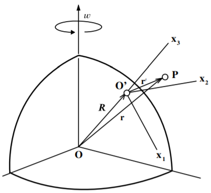
Consider a rotating frame attached to the surface of the earth as shown in Figure 12.10.1. The vector with respect to the center of the Earth $\mathbf{r}$ can be decomposed into a vector to the origin of the reference frame fixed to the surface of the Earth $\mathbf{R}$ , plus the vector with respect to this surface reference frame $\mathbf{r}^{\prime}$ .

\mathbf{r} = \mathbf{R} + \mathbf{r}^{\prime}

If the external force is separated into the gravitational term $m\mathbf{g}$ , plus some other physical force $\mathbf{F}$ , then the acceleration in the non-inertial surface frame of reference is

\mathbf{a}^{\prime} = \frac{\mathbf{F}}{m} +\mathbf{g}−(\mathbf{A} + 2\boldsymbol{\omega} \times \mathbf{v}^{\prime} + \boldsymbol{\omega} \times (\boldsymbol{\omega} \times \mathbf{r}^{\prime} ) + \boldsymbol{\dot{\omega}} \times \mathbf{r}^{\prime} )

But

\mathbf{V} = \left(\frac{d\mathbf{R}}{dt}\right)_{fixed} = \left(\frac{d\mathbf{R}}{dt}\right)_{rotating} + \boldsymbol{\omega} \times \mathbf{R} = \boldsymbol{\omega} \times \mathbf{R}

since in the rotating frame $\left(\frac{d\mathbf{R}}{dt}\right)_{rotating} = 0$ . Also the acceleration

\mathbf{A} = \left(\frac{d\mathbf{V}}{dt}\right)_{fixed} = \left(\frac{d\mathbf{V}}{dt}\right)_{rotating} + \boldsymbol{\omega} \times \mathbf{V} = \boldsymbol{\omega} \times (\boldsymbol{\omega} \times \mathbf{R})

since $\left(\frac{d\mathbf{V}}{dt}\right)_{rotating} = 0$ . Substituting this into the above equation gives

\begin{aligned} \mathbf{a}^{\prime} & = & \frac{\mathbf{F}}{m} + \mathbf{g} − (2\boldsymbol{\omega} \times \mathbf{v}^{\prime} + \boldsymbol{\omega} \times (\boldsymbol{\omega} \times [\mathbf{r}^{\prime} + \mathbf{R}]) + \boldsymbol{\dot{\omega}} \times \mathbf{r}^{\prime} ) \\ & = & \frac{\mathbf{F}}{m} + \mathbf{g} − (2\boldsymbol{\omega} \times \mathbf{v}^{\prime} + \boldsymbol{\omega} \times (\boldsymbol{\omega} \times \mathbf{r}) + \boldsymbol{\dot{\omega}} \times \mathbf{r}^{\prime} ) \end{aligned}

where $\mathbf{r}$ is with respect to the center of the Earth. This is as expected directly from equation $(12.6.8)$ . Since the angular frequency of the earth is a constant then $\dot{\omega} \times \mathbf{r}^{\prime} = 0$ . Thus the acceleration can be written as

\mathbf{a}^{\prime} = \frac{\mathbf{F}}{m} + [\mathbf{g} − \boldsymbol{\omega} \times (\boldsymbol{\omega} \times \mathbf{ r})] − 2\boldsymbol{\omega} \times \mathbf{v}^{\prime} \tag{12.52}

The term in the square brackets combines the gravitational acceleration plus the centrifugal acceleration.

A measurement of the Earth’s gravitational acceleration actually measures the term in the square brackets in Equation 12.52, that is, an effective gravitational acceleration where

\mathbf{g}_{eff} = \mathbf{g} − \boldsymbol{\omega} \times (\boldsymbol{\omega} \times \mathbf{ r})

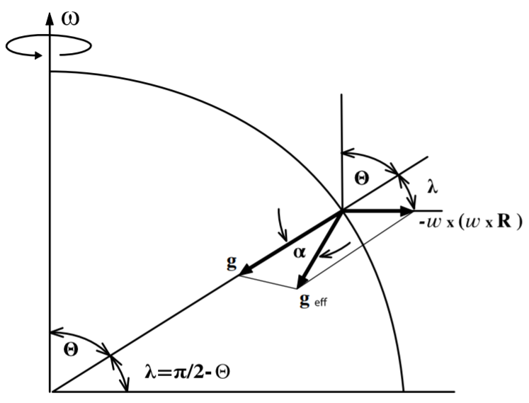
near the surface of the earth $\mathbf{r} \approx \mathbf{R}$ . The effective gravitational force does not point towards the center of the Earth as shown in Figure 12.10.2. A plumb line points, or an object falls, in the direction of $\mathbf{g}_{eff}$ . The shape of the earth is such that the Earth’s surface is perpendicular to $\mathbf{g}_{eff}$ . This is the reason why the earth is distorted into an oblate ellipsoid, that is, it is flattened at the poles.

Figure 12.10.2:Effective gravitational acceleration.

The angle $\alpha$ between $\mathbf{g}_{eff}$ and the line pointing to the center of the earth is dependent on the latitude $\lambda = \frac{\pi}{2} −\theta$ . Note that the colatitude $\theta$ is taken to be zero at the North pole whereas the latitude $\lambda$ is taken to be zero at the equator. The angle $\alpha$ can be estimated by assuming that $r^{\prime} << R$ , then the centrifugal term then can be approximated by

|\boldsymbol{\omega} \times (\boldsymbol{\omega} \times \mathbf{ r})| \approx \omega^2 R \sin \theta = \omega^2 R \cos \lambda

This is quite small for the Earth since $\omega = 0.73 \times 10^{−4}$ $rads/s$ and $R = 6371$ $km$ , leading to a correction term $\omega^2 R \cos \lambda = 0.03 \cos \lambda$ $m/s^2$ . Since

g^{horizontal}_{eff} = \omega^2 R \cos \lambda \sin \lambda

and

g^{vertical}_{eff} = g − \omega^2 R \cos^2 \lambda

Then the angle $\alpha$ between $\mathbf{g}_{eff}$ and $\mathbf{g}$ is given by

\alpha \simeq \tan \alpha = \frac{g^{horizontal}_{eff}}{g^{vertical}_{eff}} = \frac{\omega^2 R \cos \lambda \sin \lambda}{g − \omega^2 R \cos^2 \lambda}

This has a maximum value at $\lambda = 45^{\circ}$ which is $\alpha = 0.0088^{\circ}$ .

12.11: Free Motion on the Earth¶

The calculation of trajectories for objects as they move near the surface of the earth is frequently required for many applications. Such calculations require inclusion of the noninertial Coriolis force.

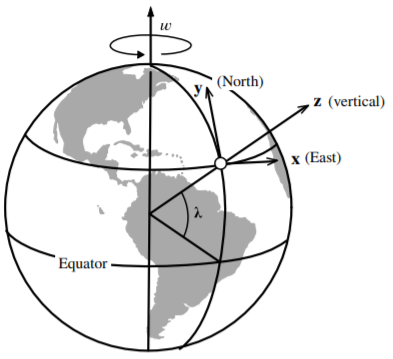
Figure 12.11.1:Rotating frame fixed on the surface of the Earth.

In the frame of reference fixed to the earth’s surface, assuming that air resistance and other forces can be neglected, then the acceleration equals

\mathbf{a}^{\prime} = \mathbf{g}_{eff} − 2\boldsymbol{\omega} \times \mathbf{v}^{\prime} \tag{12.58}

Neglect the centrifugal correction term since it is very small, that is, let $\mathbf{g}_{eff} = \mathbf{g}$ . Using the coordinate axis shown in Figure 12.11.1, the surface-frame vectors have components

\boldsymbol{\omega} = 0\widehat{\mathbf{i}^{\prime}} + \omega \cos \lambda \widehat{\mathbf{j}^{\prime}} + \omega \sin \lambda \widehat{\mathbf{k}^{\prime}}

and

\mathbf{g}_{eff} = -g\widehat{\mathbf{k}^{\prime}}

Thus the Coriolis term is

\begin{align*} 2\boldsymbol{\omega} \times \mathbf{v}^{\prime} &= 2 \begin{vmatrix} \widehat{\mathbf{i}^{\prime}} & \widehat{\mathbf{j}^{\prime}} & \widehat{\mathbf{k}^{\prime}} \\ 0 & \omega \cos \lambda & \omega \sin \lambda \\ \dot{x}^{\prime} & \dot{y}^{\prime} & \dot{z}^{\prime} \end{vmatrix} \\[4pt] &= 2 \left[ \left( \omega \dot{z}^{\prime} \cos \lambda − \omega \dot{y}^{\prime} \sin \lambda \right) \widehat{\mathbf{i}^{\prime}} + \left( \omega \dot{x}^{\prime} \sin \lambda \right) \widehat{\mathbf{j}^{\prime}} − \left( \omega \dot{x}^{\prime} \cos \lambda \right) \widehat{\mathbf{k}^{\prime}}\right] \end{align*}

Therefore the equations of motion are

m \mathbf{\ddot{r}}^{\prime} = −mg\widehat{\mathbf{k}^{\prime}} −2m[\widehat{\mathbf{i}^{\prime}} (\dot{z}^{\prime} \omega \cos \lambda − \dot{y}^{\prime} \omega \sin \lambda ) + \widehat{\mathbf{j}^{\prime}} \dot{x}^{\prime} \omega \sin \lambda − \widehat{\mathbf{k}^{\prime}} \dot{x}^{\prime} \omega \cos \lambda ]

That is, the components of this equation of motion are

\begin{align*} \ddot{x}^{\prime} &= −2\omega (\dot{z}^{\prime} \cos \lambda − \dot{y}^{\prime} \sin \lambda ) \\[4pt] \ddot{y}^{\prime} &= −2\omega \dot{x}^{\prime} \sin \lambda \notag\\[4pt] \ddot{z}^{\prime} &= −g + 2\omega \dot{x}^{\prime} \cos \lambda \end{align*}

Integrating these differential equations gives

\begin{align*} \dot{x}^{\prime} &= −2\omega (z^{\prime} \cos \lambda − y^{\prime} \sin \lambda ) + \dot{x}^{\prime}_0 \\[4pt] \dot{y}^{\prime} &= −2\omega x^{\prime} \sin \lambda + \dot{y}^{\prime}_0 \\[4pt] \dot{z}^{\prime} &= −gt + 2\omega x^{\prime} \cos \lambda + \dot{z}^{\prime}_0 \end{align*}

where $\dot{x}^{\prime}_0, \dot{y}^{\prime}_0, \dot{z}^{\prime}_0$ are the initial velocities. Substituting the above velocity relations into the equation of motion for $\ddot{x}$ gives

\ddot{x}^{\prime} = 2\omega gt \cos \lambda − 2\omega (\dot{z}^{\prime}_0 \cos \lambda − \dot{y}^{\prime}_0 \sin \lambda ) − 4\omega^2 x^{\prime}

The last term $4\omega^2x$ is small and can be neglected leading to a simple uncoupled second-order differential equation in $x$ . Integrating this twice assuming that $x^{\prime}_0 = y^{\prime}_0 = z^{\prime}_0 = 0$ , plus the fact that $2\omega gt \cos \lambda$ and $2\omega (\dot{z}^{\prime}_0 \cos \lambda − \dot{y}^{\prime}_0 \sin \lambda )$ are constant, gives

x^{\prime} = \frac{1}{3} \omega gt^3 \cos \lambda − \omega t^2 (\dot{z}^{\prime}_0 \cos \lambda − \dot{y}^{\prime}_0 \sin \lambda ) + \dot{x}^{\prime}_0 t

Similarly,

\begin{align*} y^{\prime} &= ( \dot{y}^{\prime}_0 t − \omega \dot{x}^{\prime}_0 t^2 \sin \lambda ) \\[4pt] z^{\prime} &= −\frac{1}{2} gt^2 + \dot{z}^{\prime}_0 t + \omega \dot{x}^{\prime}_0 t^2 \cos \lambda \end{align*}

Consider the following special cases;

Example 12.11.1: Free fall from rest

Assume that an object falls a height $h$ starting from rest at $t = 0$ , $x = 0$ , $y = 0$ , $z = h$ . Then

x^{\prime} = \frac{1}{3} \omega gt^3 \cos \lambda \notag

y^{\prime} = 0 \notag

z^{\prime} = h − \frac{1}{2} gt^2 \notag

Substituting for $t$ gives

x^{\prime} = \frac{1}{3} \omega \cos \lambda \sqrt{\frac{8h^3}{g}} \notag

Thus the object drifts eastward as a consequence of the earth’s rotation. Note that relative to the fixed frame it is obvious that the angular velocity of the body must increase as it falls to compensate for the reduced distance from the axis of rotation in order to ensure that the angular momentum is conserved.

Example 12.11.2: Projectile fired vertically upwards

An upward fired projectile with initial velocities $\dot{x}^{\prime}_0 = \dot{y}^{\prime}_0 = 0$ and $\dot{z}^{\prime}_0 = v_0$ leads to the relations

x^{\prime} = \frac{1}{3} \omega gt^3 \cos \lambda − \omega t^2 v_0 \cos \lambda \notag

y^{\prime} = 0\notag

z^{\prime} = −\frac{1}{2} gt^2 + v_0t\notag

Solving for $t$ when $z^{\prime} = 0$ gives $t = 0$ , and $t = \frac{2v_0}{g}$ . Also since the maximum height $h$ that the projectile reaches is related by

v_0 = \sqrt{2gh}\notag

then the final deflection is

x^{\prime} = −\frac{4}{3} \omega \cos \lambda \sqrt{\frac{8h^3}{g}} \notag

Thus the body drifts westwards.

Example 12.11.3: Motion parallel to Earth’s surface

For motion in the horizontal $x^{\prime} −y^{\prime}$ plane the deflection is always to the right in the northern hemisphere of the Earth since the vertical component of $\omega$ is upwards and thus $−2 \overrightarrow{\boldsymbol{\omega}} \times \overrightarrow{\mathbf{v}^{\prime}}$ points to the right. In the southern hemisphere the vertical component of $\omega$ is downward and thus $−2 \overrightarrow{\boldsymbol{\omega}} \times \overrightarrow{\mathbf{v}^{\prime}}$ points to the left. This is also shown using the above relations for the case of a projectile fired upwards in an easterly direction with components $\dot{x}^{\prime}_0, 0, \dot{z}^{\prime}_0$ . The resultant displacements are

x^{\prime} = \frac{1}{3} \omega gt^3 \cos \lambda − \omega t^2\dot{z}^{\prime}_0 \cos \lambda + \dot{x}^{\prime}_0 t \notag

Similarly,

y^{\prime} = −\omega \dot{x}^{\prime}_0 t^2 \sin \lambda \notag

z^{\prime} = −\frac{1}{2} gt^2 + \dot{z}^{\prime}_0 t + \omega \dot{x}^{\prime}_0 t^2 \cos \lambda \notag

The trajectory is non-planar and, in the northern hemisphere, the projectile drifts to the right, that is southerly.

In the battle of the River de la Plata, during World War 2, the gunners on the British light cruisers Exeter, Ajax and Achilles found that their accurately aimed salvos against the German pocket battleship Graf Spee were falling 100 yards to the left. The designers of the gun sighting mechanisms had corrected for the Coriolis effect assuming the ships would fight at latitudes near 50° north, not 50° south.

12.12: Weather systems¶

Weather systems on Earth provide a classic example of motion in a rotating coordinate system. In the northern hemisphere, air flowing into a low-pressure region is deflected to the right causing counterclockwise circulation, whereas air flowing out of a high-pressure region is deflected to the right causing a clockwise circulation. Trade winds on the Earth result from air rising or sinking due to thermal activity combined with the Coriolis effect. Similar behavior is observed on other planets such as the Red Spot on Jupiter.

For a fluid or gas, equation**** $(12.6.8)$ can be written in terms of the fluid density $\rho$ in the form

\rho \mathbf{a}" = −\boldsymbol{\nabla}P − \rho [2\boldsymbol{\omega} \times \mathbf{v}" − \boldsymbol{\omega} \times (\boldsymbol{\omega} \times \mathbf{r}^{\prime} )] \tag{12.68}

where the translational acceleration $\mathbf{A}$ , the gravitational force, and the azimuthal acceleration $(\boldsymbol{\dot{\omega}} \times \mathbf{r}^{\prime})$ terms are ignored. The external force per unit volume equals the pressure gradient $−\boldsymbol{\nabla}P$ while $\boldsymbol{\omega}$ is the rotation vector of the earth.

In fluid flow, the Rossby number $R_o$ is defined to be

R_o = \frac{\text{inertial force}}{\text{Coriolis force}} \approx \frac{\mathbf{a}"}{ 2\boldsymbol{\omega} \times \mathbf{v}"}

For large dimensional pressure systems in the atmosphere, e.g. $L \simeq 1000$ $km$ , the Rossby number is $R_o \sim 0.1$ and thus the Coriolis force dominates and the radial acceleration can be neglected. This leads to a flow velocity $v \simeq 10$ $m/s$ which is perpendicular to the pressure gradient $\nabla P$ , that is, the air flows horizontally parallel to the isobars of constant pressure which is called geostrophic flow. For much smaller dimension systems, such as at the wall of a hurricane, $L \simeq 50$ $km$ , and $v \simeq 50$ $m/s$ , the Rossby number $R_o \simeq 10$ and the Coriolis effect plays a much less significant role compared to the balance between the radial centrifugal forces and the pressure gradient. The same situation of the Coriolis forces being insignificant occurs for most small-scale vortices such as tornadoes, typical thermal vortices in the atmosphere, and for water draining a bath tub.

Low-pressure systems:¶

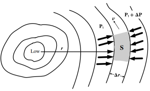
It is interesting to analyze the motion of air circulating around a low pressure region at large radii where the motion is tangential. As shown in Figure 12.12.1, a parcel of air circulating anticlockwise around the low with velocity $v$ involves a pressure difference $\Delta P$ acting on the surface area $S$ , plus the centrifugal and Coriolis forces. Assuming that these forces are balanced such that $\mathbf{a}" \simeq 0$ , then Equation 12.68 simplifies to

\frac{v^2}{r} = \frac{1}{\rho} \nabla P - 2 v \omega \sin \lambda

where the latitude $\lambda = \pi −\theta$ . Thus the force equation can be written

\frac{1}{\rho} \frac{dP}{dr} = \frac{v^2}{r} + 2v\omega \sin \lambda

It is apparent that the combined outward Coriolis force plus outward centrifugal force, acting on the circulating air, can support a large pressure gradient.

Figure 12.12.1:Air flow and pressures around a lowpressure region.

The tangential velocity $v$ can be obtained by solving this equation to give

v = \sqrt{(r\omega \sin \lambda )^2 + \frac{r}{\rho} \frac{dP}{dr}} - r\omega \sin \lambda

Note that the velocity equals zero when $r=0$ assuming that $\frac{dP}{dr}$ is finite. That is, the velocity reaches a maximum at a radius

r_{peakvel} = \frac{1}{4} (1 + \frac{1}{\rho \omega \sin \lambda} \frac{dP}{dr} )

which occurs at the wall of the eye of the circulating low-pressure system.

Figure 12.12.2:Hurricane Katrina over the Gulf of Mexico on 28 August 2005. [Published by the NOAA]

Low pressure regions are produced by heating of air causing it to rise and resulting in an inflow of air to replace the rising air. Hurricanes form over warm water when the temperature exceeds 26° $C$ and the moisture levels are above average. They are created at latitudes between 10° −15° where the sea is warmest, but not closer to the equator where the Coriolis force drops to zero. About 90% of the heating of the air comes from the latent heat of vaporization due to the rising warm moist air condensing into water droplets in the cloud similar to what occurs in thunderstorms. For hurricanes in the northern hemisphere, the air circulates anticlockwise inwards. Near the wall of the eye of the hurricane, the air rises rapidly to high altitudes at which it then flows clockwise and outwards and subsequently back down in the outer reaches of the hurricane. Both the wind velocity and pressure are low inside the eye which can be cloud free. The strongest winds are in vortex surrounding the eye of the hurricane, while weak winds exist in the counter-rotating vortex of sinking air that occurs far outside the hurricane.

Figure 12.12.2 shows the satellite picture of the hurricane Katrina, recorded on 28 August 2005. The eye of the hurricane is readily apparent in this picture. The central pressure was 90200 $N/m^2$ (902 $mb$ ) compared with the standard atmospheric pressure of 101300 $N/m^2$ (1013 $mb$ ). This 111 $mb$ pressure difference produced steady winds in Katrina of 280 $km/hr$ ( 175 $mph$ ) with gusts up to 344 $km/hr$ which resulted in 1833 fatalities.

Tornadoes are another example of a vortex low-pressure system that are the opposite extreme in both size and duration compared with a hurricane. Tornadoes may last only $\sim 10$ minutes and be quite small in radius. Pressure drops of up to 100 $mb$ have been recorded, but since they may only be a few 100 meters in diameter, the pressure gradient can be much higher than for hurricanes leading to localized winds thought to approach 500 $km/hr$ . Unfortunately, the instrumentation and buildings hit by a tornado often are destroyed making study difficult. Note that the pressure gradient in small diameter of rope tornadoes is much more destructive than for larger 1/4 mile diameter tornadoes, which results in stronger winds.

High-pressure systems:¶

In contrast to low-pressure systems, high-pressure systems are very different in that the Coriolis force points inward opposing the outward pressure gradient and centrifugal force. That is,

\frac{v^2}{r} = 2v\omega \sin \lambda − \frac{1}{\rho} \frac{dP}{dr}

which gives that

v= r\omega \sin \lambda − \sqrt{(r\omega \sin \lambda )^2 − \frac{r}{\rho} \frac{dP}{dr}}

This implies that the maximum pressure gradient plus centrifugal force supported by the Coriolis force is

\frac{r}{\rho} \frac{dP}{dr} \leq (r\omega \sin \lambda )^2

As a consequence, high pressure regions tend to have weak pressure gradients and light winds in contrast to the large pressure gradients plus concomitant damaging winds possible for low pressure systems.

The circulation behavior, exhibited by weather patterns, also applies to ocean currents and other liquid flow on earth. However, the residual angular momentum of the liquid often can overcome the Coriolis terms. Thus often it will be found experimentally that water exiting the bathtub does not circulate anticlockwise in the northern hemisphere as predicted by the Coriolis force. This is because it was not stationary originally, but rotating slowly.

Reliable prediction of weather is an extremely difficult, complicated and challenging task, which is of considerable importance in modern life. As discussed in chapter 16.8, fluid flow can be much more complicated than assumed in this discussion of air flow and weather. Both turbulent and laminar flow are possible. As a consequence, computer simulations of weather phenomena are difficult because the air flow can be turbulent and the transition from order to chaotic flow is very sensitive to the initial conditions. Typically the air flow can involve both macroscopic ordered coherent structures over a wide dynamic range of dimensions, coexisting with chaotic regions. Computer simulations of fluid flow often are performed based on Lagrangian mechanics to exploit the scalar properties of the Lagrangian. Ordered coherent structures, ranging from microscopic bubbles to hurricanes, can be recognized by exploiting Lyapunov exponents to identify the ordered motion buried in the underlying chaos. Thus the techniques discussed in classical mechanics are of considerable importance outside of physics.

12.13: Foucault pendulum¶

A classic example of motion in non-inertial frames is the rotation of the Foucault pendulum on the surface of the earth. The Foucault pendulum is a spherical pendulum with a long suspension that oscillates in the $x-y$ plane with sufficiently small amplitude that the vertical velocity $\dot{z}$ is negligible.

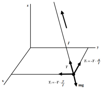
Assume that the pendulum is a simple pendulum of length $l$ and mass $m$ as shown in Figure 12.13.1. The equation of motion is given by

\mathbf{\ddot{r}} = \mathbf{g} + \frac{\mathbf{T}}{m} − 2\boldsymbol{\Omega} \times \mathbf{\dot{r}}

where $\frac{T}{m}$ is the acceleration produced by the tension in the pendulum suspension and the rotation vector of the earth is designated by $\boldsymbol{\Omega}$ to avoid confusion with the oscillation frequency of the pendulum $\omega$ . The effective gravitational acceleration $\mathbf{g}$ is given by

\mathbf{g} = \mathbf{g}_0 − \boldsymbol{\Omega} \times [\boldsymbol{\Omega} \times (\mathbf{r} + \mathbf{R})] \tag{12.78}

that is, the true gravitational field $\mathbf{g}_0$ corrected for the centrifugal force.

Assume the small angle approximation for the pendulum deflection angle $\beta$ , then $T_z = T \cos \beta \simeq T$ and $T_z = mg$ , thus $T \simeq mg$ . Then has shown in Figure 12.13.1, the horizontal components of the restoring force are

T_z = −mg \frac{x}{l}

T_y = −mg \frac{y}{l}

Since $\mathbf{g}$ is vertical, and neglecting terms involving $\dot{z}$ , then evaluating the cross product in Equation 12.78 simplifies to

\ddot{x} = −g\frac{x}{l} + 2\dot{y}\Omega \cos \theta \tag{12.81}

\ddot{y} = −g\frac{y}{l} + 2\dot{x}\Omega \cos \theta \tag{12.82}

where $\theta$ is the colatitude which is related to the latitude $\lambda$ by

\cos \theta = \sin \lambda

The natural angular frequency of the simple pendulum is

\omega_0 = \sqrt{\frac{g}{l}}

while the $z$ component of the earth’s angular velocity is

\Omega_z = \Omega \ cos \theta

Thus equations 12.81 and 12.82 can be written as

\begin{align} \notag \ddot{x} - 2\Omega_z \dot{y} + \omega^2_0 x = 0 \\ \ddot{y} - 2\Omega_z \dot{x} + \omega^2_0 y = 0 \tag{12.86} \end{align}

These are two coupled equations that can be solved by making a coordinate transformation.

Define a new coordinate that is a complex number

\eta = x + iy

Multiply the second of the coupled equations 12.86 by $i$ and add to the first equation gives

(\ddot{x} + i \ddot{y})+2i\Omega_z (\dot{x} + i\dot{y}) + \omega^2_0 (x + iy)=0 \notag

which can be written as a differential equation for $\eta$

\ddot{\eta} + 2i\Omega_z \dot{\eta} + \omega^2_0 \eta = 0 \tag{12.88}

Note that the complex number $\eta$ contains the same information regarding the position in the $x−y$ plane as equations 12.86. The plot of $\eta$ in the complex plane, the Argand diagram, is a birds-eye view of the position coordinates $(x,y)$ of the pendulum. This second-order homogeneous differential equation has two independent solutions that can be derived by guessing a solution of the form

\eta (t) = A_e^{−i\alpha t} \tag{12.89}

Substituting Equation 12.89 into 12.88 gives that

\alpha^2 − 2\Omega_z \alpha − \omega^2_o = 0 \notag

That is

\alpha = \Omega_z \pm\sqrt{\Omega^2_z + \omega^2_0}

If the angular velocity of the pendulum $\omega_0 \gg \Omega$ , then

\alpha \simeq \Omega_Z \pm \omega_0

Thus the solution is of the form

\eta (t) = e^{−i\Omega_zt} (A_+ e^{i\omega_0 t} + A_- e^{i\omega_0 t} )

This can be written as

\eta (t) = Ae^{−i\Omega_z t} \cos(\omega_0 t + \delta)

where the phase $\delta$ and amplitude $A$ depend on the initial conditions. Thus the plane of oscillation of the pendulum is defined by the ratio of the $x$ and $y$ coordinates, that is the phase angle $i\Omega_z t$ . This phase angle rotates with angular velocity $\Omega_z$ where

\Omega_z = \Omega \cos \theta = \Omega \sin \lambda

At the north pole the earth rotates under the pendulum with angular velocity $\Omega$ and the axis of the pendulum is fixed in an inertial frame of reference. At lower latitudes, the pendulum precesses at the lower angular frequency $\Omega_z = \Omega \sin \lambda$ that goes to zero at the equator. For example, in Rochester, NY, $\lambda = 43^{\circ} N$ , and therefore a Foucault pendulum precesses at $\Omega_Z = 0.682\Omega$ . That is, the pendulum precesses $245.5^{\circ}$ /day.

12.E: Non-inertial reference frames (Exercises)¶

Consider a fixed reference frame $S$ and a rotating frame $S^{\prime}$ . The origins of the two coordinate systems always coincide. By carefully drawing a diagram, derive an expression relating the coordinates of a point $P$ in the two systems. (This was covered in Chapter 2, but it is worth reviewing now.
The effective force observed in a rotating coordinate system is given by equation $(12.5.7)$ .
1. What is the significance of each term in this expression?
2. Suppose you wanted to measure the gravitational force, both magnitude and direction, on a body of mass $m$ at rest on the surface of the Earth. What terms in the effective force can be neglected?
3. Suppose you wanted to calculate the deflection of a projectile fired horizontally along the Earth’s surface. What terms in the effective force can be neglected?
4. Suppose you wanted to calculate the effective force on a small block of mass $m$ placed on a frictionless turntable rotating with a time-dependent angular velocity $\omega (t)$ . What terms in the effective force can be neglected?
A plumb line is carried along in a moving train, with $m$ the mass of the plumb bob. Neglect any effects due to the rotation of the Earth and work in the noninertial frame of reference of the train.
1. Find the tension in the cord and the deflection from the local vertical if the train is moving with constant acceleration $a_0$ .
2. Find the tension in the cord and the deflection from the local vertical if the train is rounding a curve of radius $\rho$ with constant speed $v_0$ .
A bead on a rotating rod is free to slide without friction. The rod has a length $L$ and rotates about its end with angular velocity $\omega$ . The bead is initially released from rest (relative to the rod) at the midpoint of the rod.
1. Find the displacement of the bead along the wire as a function of time.
2. Find the time when the bead leaves the end of the rod.
3. Find the velocity (relative to the rod) of the bead when it leaves the end of the rod.
Here is a “thought experiment” for you to consider. Suppose you are in a small sailboat of mass $M$ at the Earth’s equator. At the equator there is very little wind (this is known as the “equatorial doldrums”), so your sailboat is, more or less, sitting still. You have a small anchor of mass $m$ on deck and a single mast of height $h$ in the middle of the boat. How can you use the anchor to put the boat into motion? In which direction will the boat move?
Does water really flow in the other direction when you flush a toilet in the southern hemisphere? What (if anything) does the Coriolis force have to do with this?
We are presently at a latitude $\lambda$ (with respect to the equator) and Earth is rotating with constant angular velocity $\omega$ . Consider the following two scenarios: Scenario A: A particle is thrown upward with initial speed $v_0$ . Scenario B: An identical particle is dropped (at rest) from the maximum height of the particle in Scenario A. Circle all the true statements regarding the Coriolis deflection assuming that the particles have landed for a) and b), .
1. (a) The magnitude is greater in A than in B.
2. (b) The direction in A and B are the same.
3. (c) The direction in A does not change throughout flight.
If a projectile is fired due east from a point on the surface of the Earth at a northern latitude $\lambda$ with a velocity of magnitude $V_0$ and at an inclination to the horizontal of $\alpha$ , show that the lateral deflection when the projectile strikes the Earth is

d = \frac{4V^3_0}{g^2} \omega \sin \lambda \sin^2 \alpha \cos \alpha

where $\omega$ is the rotation frequency of the Earth.

Obtain an expression for the angular deviation of a particle projected from the North Pole in a path that lies close to the surface of the earth. Is the deviation significant for a missile that makes a 4800-km flight in 10 minutes? What is the ”miss distance” if the missile is aimed directly at the target? Is the miss difference greater for a 19300-km flight at the same velocity?
An automobile drag racer drives a car with acceleration $a$ and instantaneous velocity $v$ . The tires of radius $r_0$ are not slipping. Derive which point on the tire has the greatest acceleration relative to the ground. What is this acceleration?
Shot towers were popular in the eighteenth and nineteenth centuries for dropping melted lead down tall towers to form spheres for bullets. The lead solidified while falling and often landed in water to cool the lead bullets. Many such shot towers were built in New York State. Assume a shot tower was constructed at latitude $42^{\circ}$ $N$ , and that the lead fell a distance of 27 $m$ . In what direction and by how far did the lead bullets land from the direct vertical?

12.S: Non-inertial reference frames (Summary)¶

This chapter has focussed on describing motion in non-inertial frames of reference. It has been shown that the force and acceleration in non-inertial frames can be related using either Newtonian or Lagrangian mechanics by introducing additional inertial forces in the non-inertial reference frame.

Translational acceleration of a reference frame¶

In a primed frame, that is undergoing translational acceleration $\mathbf{A}$ , the motion in this non-inertial frame can be calculated by addition of an inertial force $-m\mathbf{A}$ , that leads to an equation of motion

m\mathbf{a}^{\prime} = \mathbf{F} − m\mathbf{A}

Note that the primed frame is an inertial frame if $\mathbf{A} = 0$ .

Rotating reference frame¶

It was shown that the time derivatives of a general vector $\mathbf{G}$ in both an inertial frame and a rotating reference frame are related by

\left( \frac{d\mathbf{G}}{dt}\right)_{fixed} = \left( \frac{d\mathbf{G}}{dt}\right)_{rotating} + \boldsymbol{\omega} \times \mathbf{G}

where the $\boldsymbol{\omega} \times \mathbf{G}$ term originates from the fact that the unit vectors in the rotating reference frame are time dependent with respect to the inertial frame.

Reference frame undergoing both rotation and translation¶

Both Newtonian and Lagrangian mechanics were used to show that for the case of translational acceleration plus rotation, the effective force in the non-inertial (double-primed) frame can be written as

\mathbf{F}_{eff} = m\mathbf{a}^{\prime\prime} = \mathbf{F} - m (\mathbf{A} + \boldsymbol{\omega} \times \mathbf{ V} + 2\boldsymbol{\omega} \times \mathbf{ v}^{\prime\prime} + \boldsymbol{\omega} \times (\boldsymbol{\omega} \times \mathbf{ r}^{\prime} ) + \boldsymbol{\dot{\omega}} \times \mathbf{ r}^{\prime} )

These inertial correction forces result from describing the system using a non-inertial frame. These inertial forces are felt when in the rotating-translating frame of reference. Thus the notion of these inertial forces can be very useful for solving problems in non-inertial frames. For the case of rotating frames, two important inertial forces are the centrifugal force, $−\boldsymbol{\omega} \times (\boldsymbol{\omega} \times \mathbf{r}^{\prime} )$ , and the Coriolis force $−2\boldsymbol{\omega} \times \mathbf{ v}^{\prime\prime}$ .

Routhian reduction for rotating systems¶

It was shown that for non-inertial systems, identical equations of motion are derived using Newtonian, Lagrangian, Hamiltonian, and Routhian mechanics.

Terrestrial manifestations of rotation¶

Examples of motion in rotating frames presented in the chapter included projectile motion with respect to the surface of the Earth, rotation alignment of nucleons in rotating nuclei, and weather phenomena.

Footnotes¶

For clarity sections $(12.2)$ to $(12.8)$ of this chapter adopted a naming convention that uses unprimed coordinates with the subscript $fix$ for the inertial frame of reference, primed coordinates with the subscript $mov$ for the translating coordinates, and double-primed coordinates with the subscript $rot$ for the translating plus rotating frame. For brevity the subsequent discussion omits the redundant subscripts $fix$ , $mov$ , $rot$ since the single and double prime superscripts completely define the moving and rotating frames of reference.
↩