Learning Objectives
By the end of this chapter, you should be able to:
Describe how dynamic and condenser microphones convert sound pressure into a voltage, and compare their characteristics.
Read a microphone polar pattern, and choose an appropriate pattern for a stated recording situation.
Explain how a loudspeaker converts a signal back into sound, and why a single driver cannot cover the audible range.
Explain how a magnetic pickup converts string motion into a voltage, and why pickup placement changes an electric guitar’s timbre.
Interpret a frequency-response curve, and distinguish linear distortion from nonlinear distortion.
State the sampling theorem, calculate the Nyquist frequency for a given sampling rate, and explain why 44.1 kHz was chosen for the compact disc.
Explain aliasing, predict the frequency of an aliased component, and describe the role of the anti-aliasing filter.
Relate bit depth to dynamic range through the six-decibel-per-bit rule, and explain what dither does and why it helps.
Explain how perceptual coding uses masking to discard information, and state what is and is not recoverable afterward.
Compare additive, subtractive, FM, and sampling synthesis, and identify which chapter of the book each one is an application of.
Explain how two loudspeakers produce a stereo image, and describe the cues a recording uses to place a source in space.
Introduction

Figure 15.1:Recording begins with a membrane converting pressure into motion and then voltage. Shixart1985, CC BY 2.0.
Almost all the music anybody hears has been through a microphone, a wire, and a loudspeaker. Live acoustic performance is now the exception rather than the rule, and this chapter is about the chain that has replaced it.
It is a satisfying place to end, because very little in it is new. The chain turns out to be an application of everything already established:
A microphone is a resonator with a diaphragm (Chapter 4) whose directivity is governed by size against wavelength (Chapter 2).
Digital audio rests on Fourier’s theorem (Chapter 5): a signal with no energy above some frequency can be captured by samples taken fast enough.
Perceptual coding works because masking (Chapter 7) makes much of a signal inaudible, so it need not be stored.
Synthesis is the spectrum of Chapter 5 and the source–filter model of Chapter 13, built deliberately rather than found in an instrument.
Stereo exploits the localization cues of Chapter 6, and artificial reverberation is the impulse response of Chapter 14.
There is one genuinely new idea, and it is a deep one: a continuous signal can be represented exactly by a finite list of numbers. The rest is engineering.

Figure 15.2:Technology Connections explains the 45/45 groove geometry that stores two audio channels in one mechanical trace. The construction is a compact example of turning two electrical signals into motion and back again.
Watch on YouTube: How Do Vinyl Records Hold Stereo Sound?

Figure 15.3:Ben Krasnow images a record groove directly with an electron microscope. The magnified walls make the physical waveform traced by a playback stylus visible rather than abstract.
Watch on YouTube: Vinyl LP in an Electron Microscope
15.1Microphones and Loudspeakers
Turning Pressure Into Voltage
A microphone is a pressure detector with a diaphragm, and there are two common ways to read its motion.
A dynamic microphone attaches a coil of wire to the diaphragm and suspends it in a magnetic field. Motion induces a voltage. It is rugged, needs no power, and handles very loud sources, but the coil’s mass limits its high-frequency response and its transient accuracy.
A condenser microphone makes the diaphragm one plate of a capacitor. Motion changes the capacitance and hence the voltage across it. The diaphragm can be made extremely light, so the response extends further and transients are tracked more faithfully, at the cost of needing a power supply and being more fragile.
The mechanical requirement is the same in both cases and is worth stating: the diaphragm’s resonance should be placed outside the band of interest, and it should be heavily damped, so that the microphone responds evenly rather than coloring everything with its own resonance. This is Chapter 4’s low- design philosophy, for the same reason a guitar body needs it.
Polar Patterns
A microphone’s directivity is set by whether its diaphragm is exposed to pressure on one side or both.
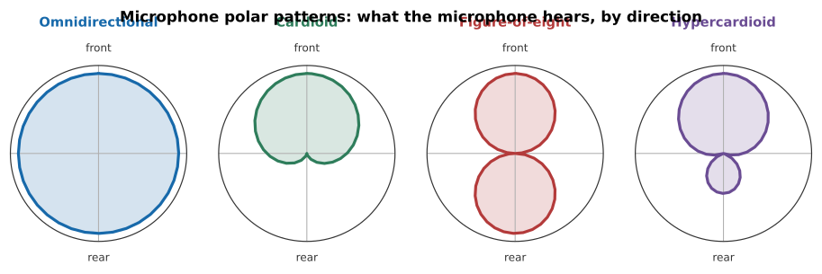
Figure 15.4:The four standard patterns. Omnidirectional responds to pressure alone and hears everything equally. Figure-of-eight responds to the pressure difference across the diaphragm, so it is deaf at the sides. Cardioid is the sum of the two, giving a rear null. Hypercardioid is a different mixture, trading a small rear lobe for a narrower front.
The choice is a practical one. A cardioid rejects the room and the audience, which suits a close-miked instrument in a poor room. An omnidirectional captures the room, which suits a good hall. A figure-of-eight rejects sound from the sides, and is used to isolate two instruments facing each other.
Loudspeakers, Drivers, and Crossovers
A loudspeaker runs the microphone backwards: current through a coil in a magnetic field produces force, which moves a cone, which pushes air.
It faces a problem Chapter 2 identified. Directivity depends on the source’s size compared with the wavelength, and a single driver has one size while music spans a factor of a thousand in wavelength. A driver large enough to move air at 40 Hz beams badly at 4 kHz; one small enough to radiate 10 kHz evenly cannot shift enough air to produce bass at all.
The solution is multiple drivers, a woofer, sometimes a midrange, and a tweeter, with a crossover network dividing the signal between them. The crossover is itself a compromise, since the drivers must blend through the handover region without canceling, and crossover design is much of what distinguishes loudspeakers.
The low-frequency problem is attacked separately. A cone radiates from both faces, in opposite phase, so at long wavelengths the front and rear outputs meet around the edge and cancel. An enclosure prevents that. A sealed box is simple and well-behaved; a bass-reflex box adds a tuned port, a Helmholtz resonator (Chapter 4), that reinforces the bottom octave at the cost of a steeper roll-off below it.

Figure 15.5:Branch Education follows an electrical signal through the magnet and voice coil to the moving cone and the pressure wave radiated into the room. The cutaway view shows how the components described above fit together.
Watch on YouTube: How Do Speakers Work?
Electromagnetic Pickups: A Different Transducer
A microphone reads pressure in the air; an electric guitar’s pickup reads the string directly, and it works on a different principle entirely.
A magnetic pickup is a coil of wire wound around a permanent magnet. The magnet’s field passes through the string, provided the string is ferrous (steel, or steel-wound), and magnetizes a section of it. As the string vibrates, it disturbs that field, and the changing flux through the coil induces a voltage by Faraday’s law. No power supply, no diaphragm: the string is the diaphragm.
One consequence is easy to miss. Because the induced voltage depends on the rate of change of flux, the pickup’s output is proportional to the string’s velocity, not its displacement. This is the same distinction Chapter 10 draws between the bridge force a soundboard responds to and the string’s actual shape.
A second consequence is audible on every electric guitar. A pickup samples the string’s motion at one fixed point along its length, and Chapter 10 showed that the plucking or driving point determines which harmonics are strong: a point that is a node for some harmonic contributes almost nothing at that harmonic to the output. A neck pickup, positioned nearer the string’s midpoint, favors the fundamental and sounds warm; a bridge pickup, positioned near a region where high harmonics have their antinodes, emphasizes them and sounds bright and biting. Switching pickups, or blending them, is comb filtering by another name, chosen by ear rather than calculated.
Not every electric or amplified string instrument uses this principle. A piezoelectric pickup, common on acoustic-electric guitars, basses, and violins, is mounted under the bridge saddle and generates a voltage from mechanical stress rather than magnetic flux, so it works on nylon or gut strings that a magnetic pickup cannot see at all, and it responds to the bridge’s motion rather than the string’s.
15.2Signals and Their Imperfections
Frequency Response
The frequency response of any component is its gain against frequency. A perfect one would be flat across the audible range.
Nothing is. Loudspeakers are the worst offenders by a wide margin: even a good one varies by several decibels across its range, while a competent amplifier is flat to a fraction of a decibel. In any audio chain, the transducers, microphone, loudspeaker, and the room, are where essentially all of the frequency-response error lives.
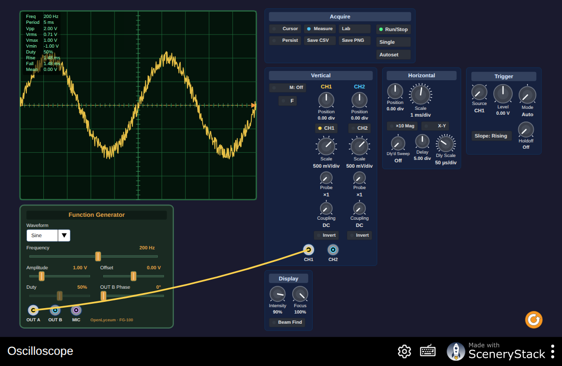
Figure 15.6:An oscilloscope with a signal generator behind it. Set a sine wave and measure its period from the screen; then add a second channel and look at what a sum looks like. This is the instrument the laboratory exercises in Laboratory Exercises assume; fluency with it helps before meeting a real one.
Interactive simulation: Oscilloscope
Linear and Nonlinear Distortion
Two kinds of error, and conflating them causes endless confusion.
Linear distortion changes the balance of the frequencies present. A frequency-response error is linear distortion, and so is a phase shift. It adds nothing new: whatever comes out was in the input, at a different level. It can, in principle, be corrected by an inverse filter, which is what room equalization attempts.
Nonlinear distortion creates frequencies that were not present in the input. If the output is not proportional to the input, Chapter 3’s superposition fails, and a sum of two tones produces components at sums and differences of their frequencies. This cannot be corrected by filtering, because the new components are entangled with the wanted ones.
Two measures are quoted. Total harmonic distortion measures added harmonics of a single input tone. Intermodulation distortion measures the sum and difference components from two tones, and is the more revealing, because harmonics of a musical note are at least musically related to it while intermodulation products are not.
Noise and Dynamic Range
Every stage adds noise, and the dynamic range of a system is the span between its noise floor and the level at which it distorts.
The requirement follows from Chapter 7. An orchestra spans about 50 dB from pianissimo to fortissimo, and a good hall has a background around 25 dB SPL. A system with 90 dB of dynamic range has ample margin; one with 50 dB does not, and either the quiet passages disappear into hiss or the loud ones distort.
15.3Digital Audio
Sampling and the Nyquist Frequency
Here is the central result.
The sampling theorem. A signal containing no frequencies above is completely determined by samples taken at any rate greater than .
Not approximately. Completely. The samples contain every bit of information in the original, and the original can be reconstructed from them exactly.
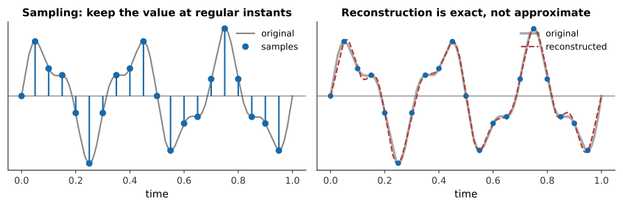
Figure 15.7:Sampling and reconstruction. The right panel is the surprising half: the reconstruction is not a join-the-dots approximation but an exact recovery, obtained by summing a function centered on each sample. Nothing has been lost.
The Nyquist frequency is half the sampling rate: the highest frequency a given rate can represent.
The compact disc samples at 44.1 kHz, giving a Nyquist frequency of 22.05 kHz, comfortably above the 20 kHz limit of hearing. The awkward number is historical: early digital recorders stored data on video tape, and 44.1 kHz was what fitted the existing video line rates.
Aliasing and the Anti-Aliasing Filter
The theorem’s condition, no frequencies above Nyquist, is not optional, and violating it is not a gentle degradation.
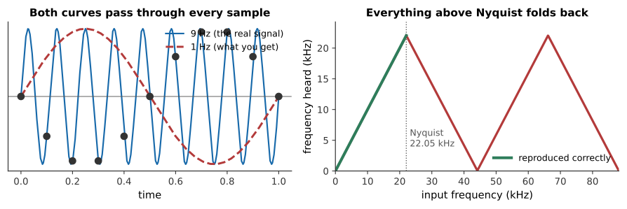
Figure 15.8:Left: a 9 Hz signal sampled at 10 Hz produces exactly the same samples as a 1 Hz signal. Nothing in the data can distinguish them. Right: the general rule, every frequency above Nyquist is folded back below it, reappearing as a different frequency altogether.
The consequence is severe. Aliased components are not a distortion of the original; they are new frequencies at unrelated pitches, and once the samples are taken there is no way to remove them.
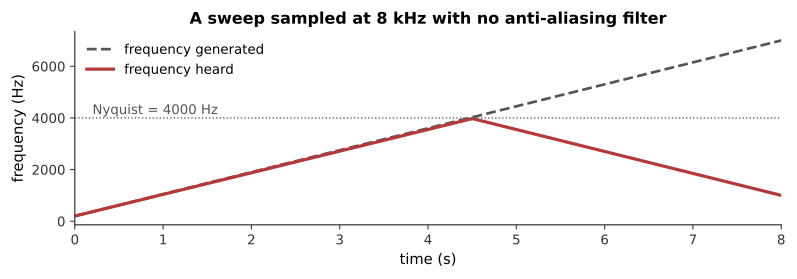
Figure 15.9:A sweep from 200 Hz to 7 kHz, synthesized at 8 kHz with no anti-aliasing filter. Above 4 kHz the tone folds back and descends. Nothing in the generator ever descends; what you are hearing is the folding diagram above, made audible.
What you hear: A rising tone that climbs for about half the clip, then turns round and descends, and then turns again, even though the generator is sweeping steadily upward the whole time.
Listen: Aliasing Sweep
The cure is to filter before sampling. An anti-aliasing filter removes everything above Nyquist while the signal is still continuous, so the theorem’s condition is satisfied. It must come first, after sampling, the aliased components are indistinguishable from real ones.
This is the technical reason for sampling faster than strictly necessary. A perfect filter is impossible, so a real one needs a transition band, and the gap between 20 kHz and 22.05 kHz is where the CD’s filter does its work.
Quantization, Bit Depth, and Dither
Sampling discretizes time. Quantization discretizes amplitude, rounding each sample to the nearest of a finite set of levels, and unlike sampling it is not lossless.
The error is bounded by half a level, and the resulting dynamic range is
with the number of bits: the useful rule being about 6 dB per bit. A 16-bit CD gives 98 dB, comfortably beyond any listening room. A 24-bit studio format gives 146 dB, which is far beyond any microphone, and exists to provide headroom during processing rather than for final delivery.
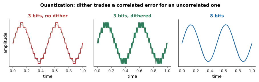
Figure 15.10:Quantization at three bit depths. The middle panel shows what dither does: adding a small amount of noise before quantizing.
Dither seems perverse, deliberately adding noise to improve quality, and it is one of the more elegant ideas in signal processing. Without it, the quantization error is correlated with the signal: it follows the waveform, producing harmonic distortion that is worst on quiet passages, exactly where it is least welcome. Adding a small random noise decorrelates the error, converting it into a steady, signal-independent hiss.
The total error energy is slightly greater. The audible result is much better, because the ear is far more tolerant of steady noise than of signal-dependent distortion.
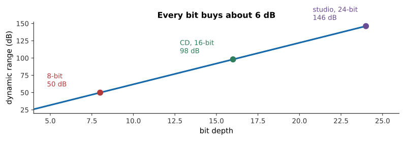
Figure 15.11:The same note at three quantizations. Listen to the tails. The undithered version does not merely get noisy as it decays, it becomes distorted and granular, because the error is following the signal. The dithered version has more noise overall and sounds better, which is the whole argument for dither.
What you hear: The same decaying note three times. The first is clean. The second is clean at first and then breaks up into a gritty, buzzy crackle as it fades. The third has an audible steady hiss but fades away smoothly.
Listen: 16-bit, 6-bit undithered, 6-bit dithered
15.4Perceptual Coding
Using Masking to Throw Things Away
A CD carries about 1.4 megabits per second. An MP3 at 128 kbit/s carries a tenth of that and most listeners cannot reliably tell them apart. Something is being thrown away, and the question is what.
The answer comes straight from Chapter 7. If a component is masked, the listener cannot hear it; so it does not need to be stored.
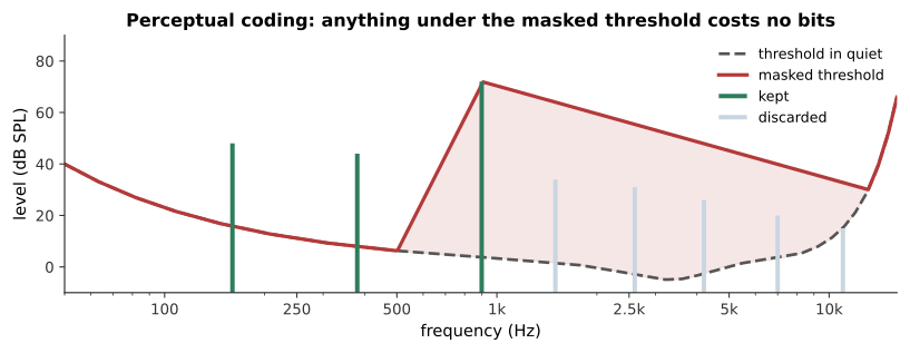
Figure 15.12:How a codec decides. It computes the masked threshold, the level below which nothing is audible, given what else is present, and discards everything under it. The discarded components are not approximated or attenuated; they are simply not stored.
A codec works in short blocks, and for each one it transforms to the frequency domain, computes the masked threshold from a psychoacoustic model, allocates bits so that quantization noise in each band sits just below that threshold, and encodes the result.
Figure 15.13:A loud 900 Hz tone with three quiet partials, and the same with those partials deleted. They are hard to tell apart because the partials were masked, they were present in the signal and absent from your perception of it, so removing them changed nothing you could hear.
What you hear: Two tones that sound essentially identical. The second has had three quiet partials removed entirely, and it is very hard to hear any difference at all.
Listen: All components, Masked components removed
What a Lossy Codec Keeps
The bit allocation follows the ear’s own priorities, and the consequences are visible in what codecs are good and bad at.
Low frequencies get more bits, because the critical bands are narrower there and masking is less generous.
Steady tones compress well; sharp transients compress badly. A transient needs short blocks to be located in time, and short blocks have poor frequency resolution (Chapter 5’s trade-off, in a new guise). Applause, castanets, and harpsichords are the classic hard cases, and codecs switch block length dynamically for that reason.
Stereo is exploited. Much of the two channels is common, and encoding a sum and a difference is cheaper than encoding both.
What Is Lost for Good
Two honest caveats.
Lossy is lossy. The discarded information is gone. Re-encoding an MP3, decoding and re-encoding, as happens when a file is edited or converted, applies the model to a signal that has already been altered, and the errors accumulate. Archives should be stored losslessly.
The model can be wrong. The masking model is built on average listeners and typical signals. Unusual material can defeat it, and the artifacts are characteristic: pre-echo, where a transient’s quantization noise is spread backwards in time and becomes audible before the event that caused it, and a swirling, watery quality in cymbals where the codec’s decisions change from block to block.
15.5Synthesis
Additive Synthesis: Fourier in Reverse
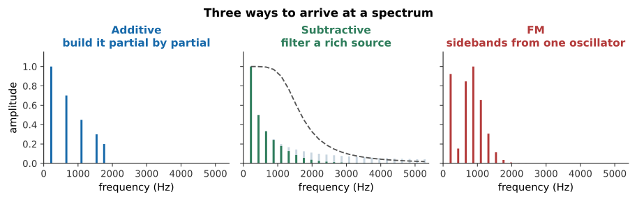
Figure 15.14:Three routes to a spectrum. Additive builds it partial by partial, subtractive carves it out of a rich source, and FM generates a whole family of sidebands from two oscillators.
Additive synthesis builds a sound by summing sinusoids with individually chosen amplitudes and envelopes. It is Fourier’s theorem run backwards, and it can produce any periodic sound whatever.
Its weakness is not sound quality but control. A realistic instrument needs dozens of partials, each with its own time-varying amplitude, which is hundreds of parameters per note. The Hammond organ is additive synthesis with nine drawbars, and it sounds like a Hammond organ rather than like anything else, which says something about how far nine partials get you.
Subtractive Synthesis and the Source–Filter Model Again
Subtractive synthesis starts with a spectrally rich source, a sawtooth, a square, or noise, and removes what is not wanted with a filter.
This is exactly the source–filter model of Chapter 13, and the analogy is not loose: the oscillator is the vocal folds and the filter is the vocal tract. A resonant low-pass filter with a swept cutoff is imitating a formant, and a synthesizer player sweeping a filter is doing what a singer does moving their tongue.
It dominated analog synthesis because it is efficient. Two or three controls, cutoff, resonance, and an envelope on the cutoff, produce an enormous range of usable timbres, where additive synthesis needs hundreds.
Figure 15.15:The same pitch by three methods. The subtractive example’s filter sweep and the FM example’s falling modulation index are doing the same job, making the spectrum change over the course of the note, which Chapter 5 identified as the thing static synthesis most obviously lacks.
What you hear: Three tones at the same pitch. The first is hollow and organ-like. The second starts bright and darkens as its filter closes. The third is metallic and bell-like, becoming purer as it decays.
Listen: Additive, Subtractive, FM
FM Synthesis and Sampling
FM synthesis, discovered by John Chowning in 1967 and commercialized in the Yamaha DX7 in 1983, uses one oscillator to modulate another’s frequency.
Modulating a carrier at with a modulator at produces sidebands at
whose amplitudes are Bessel functions of the modulation index: the ratio of frequency deviation to modulator frequency. Raising the index spreads energy into more sidebands.
Two features made it commercially decisive. It is cheap: two oscillators produce dozens of partials, which mattered enormously with 1980s hardware. And the index can be varied over the note, so a falling index makes a bright attack settle to a pure sustain, precisely the behavior of a struck bar or a bell (Chapter 12). FM’s metallic and bell-like sounds were therefore much better than anything else available at the time.
If and are in a simple ratio, the sidebands land on a harmonic series and the sound is pitched. If not, they do not, and the result is inharmonic, which is the same distinction Chapter 12 drew between a string and a gong, arrived at from the other direction.
Sampling, playing back recordings of real instruments, sidesteps synthesis entirely and dominates commercial music production. Its difficulty is that a sample is one note, at one dynamic, at one moment; covering an instrument’s range requires many, and the couplings Chapter 10 described: a piano played louder is also brighter, must be reproduced by switching between samples recorded at different dynamics. A sampler that changes only loudness sounds instantly wrong.
15.6Space in a Recording
Two Speakers, One Image
Two loudspeakers can produce a sound that appears to come from a point between them, where nothing is.
The mechanism is summing localization. Identical signals from both give a phantom image at the center. Making one louder: an intensity difference, pulls the image toward it, and about 15–18 dB places it fully at one speaker. Making one earlier: a time difference, does the same, with about 1 ms sufficing.
Both work because they crudely reproduce what a real source would do at the two ears.
Localization Cues and the HRTF
Real localization uses three cues, and a recording can only approximate them.
Interaural time difference dominates below about 1.5 kHz: a sound from the left reaches the left ear up to 0.7 ms sooner.
Interaural level difference dominates above: the head shadows the far ear, by up to 20 dB at high frequencies.
Spectral cues from the pinna resolve front from back and above from below (Chapter 6), and they are the only cue that can. The whole direction-dependent filter is called the head-related transfer function.
Ordinary stereo reproduces only the first two, and only crudely, so a stereo image is a line between the speakers rather than a space. Binaural recording, made with microphones in the ears of a dummy head, captures the HRTF as well, and over headphones produces a startling sense of height and behindness. Its limitation is that it encodes somebody else’s ears, and that it breaks as soon as the listener turns their head, hence the rise of head-tracked systems.
Reverberation, Real and Artificial
Every recording must decide how much room to include, and the decision cannot be postponed: reverberation recorded into a track cannot be removed.
Modern practice therefore records dry, close-miked, in a treated room, and adds reverberation afterwards. Two methods.
Algorithmic reverberation builds a decaying field from networks of delays and filters. It is efficient, adjustable in every parameter, and can produce spaces that could not be built.
Convolution reverberation uses a measured impulse response of a real hall and convolves the dry signal with it (Chapter 14). It sounds exactly like that hall, from that seat, because it is that hall’s response, at the cost of being fixed, since the response encodes one source position, one listening position, and one room.
And so the book’s last idea is one of its first. Chapter 3 established superposition; Chapter 14 established that a room’s effect is completely described by its impulse response; and convolution reverb is nothing but those two facts applied at forty-four thousand samples per second. A recording engineer placing a soloist in the Concertgebouw is doing linear superposition, very fast.
15.7Summary
Dynamic microphones use a coil and magnet; condensers use a variable capacitor and a much lighter diaphragm. Both want a well-damped resonance outside the audio band, low , as in Chapter 4.
Polar patterns follow from whether the diaphragm senses pressure (omnidirectional) or pressure difference (figure-of-eight); cardioid is their sum. Every pressure-difference microphone shows proximity effect.
Loudspeakers need multiple drivers, because directivity depends on size against wavelength and music spans a factor of a thousand in wavelength. Enclosures prevent front-to-back cancellation; a bass-reflex port is a Helmholtz resonator.
A magnetic pickup induces a voltage from a ferrous string’s motion directly, no diaphragm required; its output tracks string velocity, and its fixed sampling point along the string means placement (neck versus bridge) reshapes the harmonic balance, the same driving-point physics as Chapter 10.
Linear distortion rebalances existing frequencies and is in principle correctable; nonlinear distortion creates new ones and is not.
The sampling theorem: a signal with no energy above is completely determined by samples at any rate above . Reconstruction is exact.
Aliasing folds everything above the Nyquist frequency back below it, producing new frequencies at unrelated pitches. The anti-aliasing filter must act before sampling, because afterwards nothing can distinguish an alias from a real component.
Quantization gives about 6 dB of dynamic range per bit. Dither adds noise before quantizing, converting signal-correlated distortion into steady hiss, more total error energy, much better sound.
Perceptual coding discards masked components, which by definition cannot be heard. It struggles with transients, because locating them in time requires short blocks and short blocks resolve frequency poorly.
Additive synthesis specifies every partial; subtractive filters a rich source and is the source–filter model again; FM generates Bessel-weighted sidebands from two oscillators, giving inharmonic spectra cheaply.
Stereo works by summing localization, reproducing interaural time and level differences but not the pinna cues that distinguish front from back. Convolution reverb is superposition plus a measured impulse response.
15.8Check Your Understanding
Five short, auto-graded questions cycle within one compact activity, using five different response styles.
Multiple choice. Where must an anti-aliasing low-pass filter act: before sampling, after sampling, or only during playback?
True or false. Dither improves low-level digital sound by reducing the total error energy introduced during quantization.
Drag the words. Match dynamic and condenser microphones and omnidirectional and figure-of-eight patterns to their operating principles.
Fill in the blank. At roughly 6 dB per bit, ideal 16-bit audio provides about ___ dB of dynamic range.
Mark the words. Identify the two processes that create new frequency components: “FM synthesis generates sidebands, and nonlinear distortion creates new frequencies; subtractive filtering only rebalances frequencies already present.”
15.9Conceptual Questions
Explain why a condenser microphone tracks transients better than a dynamic one.
Explain why an omnidirectional microphone shows no proximity effect while a cardioid does.
Explain why a single loudspeaker driver cannot reproduce the whole audible range, referring to source size and wavelength.
A guitarist blends a neck and a bridge pickup and notices the tone changes even though nothing about the string or the amplifier has changed. Explain why, referring to the driving-point argument of Chapter 10.
Distinguish linear from nonlinear distortion, and explain why only one of them can in principle be corrected.
State the sampling theorem, and explain what is surprising about the word “completely” in it.
Explain why an anti-aliasing filter must be applied before sampling rather than after.
Explain why adding noise before quantizing improves the perceived quality, given that it increases the total error.
Explain why perceptual codecs handle a sustained organ chord better than applause.
15.10Problems
Solution to Exercise 15.1 #
(a) kHz.
(b) Anything below 24 kHz.
(c) Frequencies above Nyquist fold back:
Therefore a 30 kHz component, inaudible in itself, appears as an 18 kHz component, which is audible to many listeners and is not in the original at all.
Solution to Exercise 15.2 #
Solution to Exercise 15.3 #
Using dB:
(a) dB.
(b) dB.
(c) dB.
(d) The hall requires dB. The 8-bit system is inadequate; 16-bit has 18 dB of margin and is sufficient; 24-bit is far beyond any microphone’s own noise floor and exists to give headroom during processing rather than for delivery.
Solution to Exercise 15.4 #
(a) .
(b) .
(c) Masking (Chapter 7). At any instant, most of the spectral detail in a musical signal lies below the masked threshold set by the louder components, and a listener cannot hear it. A codec computes that threshold and spends bits only above it.
Therefore the discarded is not “detail the listener might miss”; it is information the auditory system was never going to receive. The compression is therefore much more effective than a general-purpose lossless compressor, which manages only about on audio.
Solution to Exercise 15.5 #
(a) Sidebands are at :
Negative frequencies fold back with inverted phase, so the set is 440, 880, 1320, 1760, 2200 Hz.
(b) Yes, every component is a multiple of 440 Hz, so the result is a harmonic series and the sound is clearly pitched.
(c) With Hz: ; ; . The set is 129, 182, 440, 493, 751, 1062, 1373 Hz, no common fundamental, so the result is inharmonic and bell-like.
Therefore the ratio decides whether FM produces a pitched instrument or a percussion instrument, which is exactly the distinction of Chapter 12 reached from the other direction.
Solution to Exercise 15.6 #
(a) Full deflection to one speaker takes about 15–18 dB, so 6 dB places the image roughly a third of the way from center to the left speaker.
(b) Full deflection takes about 1 ms, so a comparable shift needs roughly 0.3 ms of delay on the right channel.
(c) Both crudely reproduce what a real source to the left would produce at the ears: it would arrive sooner and louder at the left ear. The auditory system integrates the two loudspeakers’ outputs and infers a direction consistent with the cues it receives.
Therefore intensity and time panning are interchangeable to a first approximation, and are used interchangeably, though they are not identical, and combining them inconsistently produces an unstable image.
Solution to Exercise 15.7 #
(a) Setting , so :
(b) Somewhere around 1.5–2.5 kHz.
(c) The crossover should hand over before the woofer starts beaming: that is, at or below about 1.4 kHz by the calculation above, though in practice a little above is tolerated. It must not be so low that the tweeter is asked to move air at frequencies where its small cone cannot produce enough displacement without distorting.
Therefore the choice is squeezed from both sides, and 2 kHz is the usual compromise, which is unfortunate, since it sits in the region where hearing is most sensitive and where the ear most easily detects the discontinuity.
Solution to Exercise 15.8 #
At exactly 40 kHz the Nyquist frequency is 20 kHz, so the anti-aliasing filter would need to pass 20 kHz unattenuated and stop everything above 20 kHz completely: an infinitely steep transition, which is impossible.
At 44.1 kHz the Nyquist frequency is 22.05 kHz, leaving a transition band from 20 to 22.05 kHz. Expressed as a slope requirement, the filter must fall from passband to stopband over
under a tone and a half, still a demanding filter, but a buildable one.
Therefore the extra 4.1 kHz buys the filter room to work. The precise figure is historical rather than acoustic: early digital audio was stored on video recorders, and 44.1 kHz is what fell out of the available line and field rates.
Solution to Exercise 15.9 #
(a) Sums and differences and their combinations:
(b) Yes, in this case, all of them. The two inputs are a perfect fifth apart (), so they are harmonics 2 and 3 of a common fundamental at 110 Hz, and every intermodulation product is therefore also a harmonic of 110 Hz.
(c) That is precisely why the sound works. For consonant intervals the distortion products fall on the existing harmonic series and add weight rather than dissonance. Power chords, built on fifths, sound so good through a distorted amplifier for that reason.
For a more complex chord, a major third, say, the products do not all fall on a common series, and the result is muddy. Guitarists know this as the rule that distorted chords should be kept to two notes, and the reason is the arithmetic above.
Solution to Exercise 15.10 #
(a) samples.
(b) A 4-minute track is samples, and each output sample requires one multiply per impulse-response sample:
(c) Two trillion multiplications per channel is far too many for real time on modest hardware.
The remedy is the convolution theorem: convolution in time is multiplication in frequency, so the operation can be done by transforming both signals, multiplying, and transforming back. Using the fast Fourier transform this reduces the cost by roughly a factor of , which here is about 104, bringing two trillion operations down to a few hundred million, which is entirely practical.
Therefore convolution reverb is possible because of Fourier’s theorem, which is a pleasing place for a book that began with a vibrating string to end.
Solution to Exercise 15.11 #
With bits there are levels. Let the full-scale signal be a sine of amplitude , so peak-to-peak it spans and each quantization step is
The quantization error is uniformly distributed over , so its mean square is
The signal’s mean square is . The signal-to-noise ratio is therefore
In decibels:
Therefore each additional bit doubles the number of levels, halves the step, and buys dB, and the 1.76 dB offset comes from the ratio between a sine’s mean square and a uniform error’s.
Solution to Exercise 15.12 #
(a) At 30 cm the microphone is well inside the critical distance, so the direct sound dominates heavily, this is a dry, close recording.
(b) At 2.5 m the microphone is beyond the critical distance, so the reverberant field dominates and the recording captures mostly room.
(c) For most modern production, the close position. A dry recording can have reverberation added afterwards by convolution (Chapter 14), and the amount can be chosen at mixing time. Reverberation recorded into a track cannot be removed.
Two caveats. The close position will show proximity effect, boosting the bass substantially, which must be corrected or exploited. And if the room is genuinely good, a fine hall, the distant position captures something an artificial reverberation cannot quite reproduce. Classical recording still uses distant main pairs for that reason.
Solution to Exercise 15.13 #
A codec works on blocks. Within each block it transforms to the frequency domain, decides how much quantization noise each band can carry without being audible, and quantizes accordingly.
The quantization noise it introduces is spread uniformly over the whole block, because the quantization happens in the frequency domain and a frequency-domain error has no localization in time.
Now consider a block containing a castanet click: silence for most of its duration, then a loud transient. The masking model computes a threshold from the block’s overall spectrum, which the loud transient dominates, so a generous amount of noise is permitted. That noise is then spread across the entire block, including the silent part before the click.
The result is a burst of noise audible in the silence preceding the transient: pre-echo.
Chapter 5’s trade-off is what makes this unavoidable in principle: locating the transient precisely in time requires a short block, and a short block resolves frequency poorly, which degrades the masking model. Codecs respond by switching block length dynamically, using short blocks when a transient is detected and long ones otherwise, which mitigates the problem without eliminating it.
Solution to Exercise 15.14 #
(a) Pitch-shifting by resampling scales every frequency in the recording, including the resonances of the soundboard and body. But those resonances are properties of the instrument and do not move when the pitch changes, they are formants, in the sense of Chapter 13. Shifting an octave moves them an octave too, and the result sounds like a smaller instrument. Shifting down produces the well-known “munchkinization” in reverse.
The note’s duration also scales, so the shifted note decays twice as fast, which is wrong, since a real piano’s high notes decay faster for reasons of string mass, not by a factor of exactly two.
(b) Chapter 10 showed that a piano hammer’s felt is nonlinear: struck harder, contact time shortens and more high harmonics survive. A piano played louder is brighter, not merely louder. A sampler with one dynamic level can only change the volume, so a fortissimo sounds like a pianissimo turned up, instantly recognizable as wrong.
(c) Both failures come from the same source: an instrument is not a single sound with adjustable pitch and volume. Its spectrum depends on the note and on the dynamic, through mechanisms Chapter 10 described.
Therefore good samplers record many notes across the range, at several dynamic levels, and cross-fade between them. A convincing sampled piano therefore runs to many gigabytes.