Learning Objectives¶
By the end of this chapter, you should be able to:
Distinguish free vibration at a natural frequency from forced vibration at a driving frequency.
Sketch the response of a driven oscillator against driving frequency, and identify the resonance peak, its height, and its width.
Explain why a system driven at resonance builds up a large amplitude, in terms of energy delivered in step with the motion.
Relate damping to the sharpness of a resonance, define the quality factor , and calculate it from the bandwidth of a measured response curve.
Explain the trade-off a Q value represents for an instrument: a sharp resonance is loud and selective, a broad one is even and responsive.
Define a normal mode, and explain why a system with degrees of freedom has of them.
Explain how an arbitrary motion of a vibrating system can be written as a combination of its normal modes, and why the modes are the natural description.
Identify the resonator in a guitar, a violin, a trumpet, and the human voice, and describe what each contributes to the sound.
Introduction¶
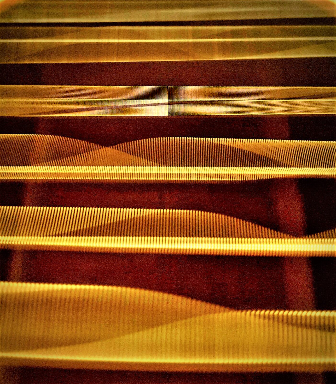
Figure 4.1:A guitar is a compact collection of resonators: strings, plates, an enclosed air cavity, and the room beyond them. Here the strings themselves are doing it, each blurred band the shape of one string’s vibration. Matt Stetzel, CC BY 4.0.
Chapter 3 established that a string fixed at both ends can only vibrate at certain frequencies. That is a statement about what the string will do if left alone. This chapter is about what happens when it is not left alone, when something drives it.
The answer is the single most useful idea in instrument design. Drive a system at one of its natural frequencies and it responds enormously; drive it anywhere else and it barely responds at all. That selectivity is resonance, and every instrument in this book depends on it twice over: once to choose which frequency will sound, and again to get that frequency out into the room loudly enough to hear.
Two ideas run through the chapter, and they turn out to be the same idea seen from two sides.
The first is the trade-off. A sharply tuned resonator responds hugely, but only to a narrow band of frequencies, and it rings for a long time after the driving stops. A broadly tuned one responds modestly, to almost anything, and stops as soon as the driving does. An instrument maker must choose, and different instruments choose differently.
The second is the normal mode. A real object does not have one natural frequency; it has many, each with its own characteristic shape. The remarkable fact, and the reason Chapter 5 can exist, is that any motion whatsoever of such an object is a sum of its modes.
4.1Free Vibration and Natural Frequency¶
Natural Frequencies of Real Objects¶
Displace something and let go, and it vibrates at its natural frequency. A mass on a spring does it at ; a string fixed at both ends does it at ; a wine glass, a tuning fork, a wooden bar, a column of air, a bridge, and a building all do it at frequencies set by their own stiffness and mass.
This is free vibration: no one is driving it, the amplitude decays as Chapter 1 described, and the frequency is whatever the object’s construction dictates.
Notice that damping barely changes the frequency. A lightly damped oscillator rings at almost exactly the frequency it would have had with no damping at all: the correction is of order , and for any above about 5 it is negligible. A guitar string therefore sounds the same note whether you let it ring or mute it quickly, and the formulas of Chapter 3, which ignored damping entirely, were safe to write down.
Why Every Object Has More Than One¶
A mass on a spring has exactly one natural frequency, because it has exactly one way to move: the mass goes left or it goes right.
A string is different. It can bow out in one arch, or in two, or in three, and each of those shapes has its own frequency. The number of natural frequencies is the number of independent ways the object can move, its number of degrees of freedom, and for anything continuous, that number is unlimited.
This matters for a reason that will not be obvious yet: it means the word “resonance” is almost always plural. A guitar body does not have a resonance; it has dozens, and the shape of the resulting response curve is what a luthier is actually adjusting when they thin a brace by a fraction of a millimeter.
4.2Driven Oscillation and Resonance¶
Driving an Oscillator Off and On Resonance¶
Now apply a force that oscillates at a frequency of your choosing, and ask how large a response you get.
After any initial transient dies away, the system settles into oscillating at the driving frequency, not at its own. That is worth stating clearly because it is counterintuitive: the driven system abandons its natural frequency and does what it is told. What its natural frequency controls is not the frequency of the response but its size.
Drive it very slowly, far below : the mass simply follows the force. The response is small and in step with the drive.
Drive it at : each push arrives exactly when it helps, cycle after cycle, and the amplitude builds far beyond anything the force could achieve on its own.
Drive it far above : the mass cannot keep up. It barely moves, and what motion there is lags half a cycle behind.
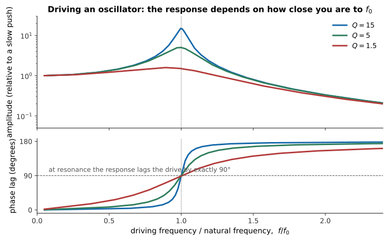
Figure 4.2:The response of a driven oscillator as the drive frequency sweeps back and forth through resonance. Left: a constant-strength force drives the oscillator shown by the green curve. Its motion grows dramatically near , and its timing shifts from following the force to opposing it. Right, top: the amplitude for three amounts of damping. Right, bottom: the corresponding phase lag. At resonance the response lags the drive by exactly , whatever the damping, which is the precise statement of “pushing at the right moment”.
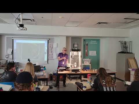
Figure 4.3:In this University of British Columbia outreach demonstration, a loudspeaker drives a wine glass at its natural frequency. High-speed footage shows the resonant motion growing until the glass fails: a vivid example of a small periodic force transferring energy efficiently when its frequency is correctly matched.
Watch on YouTube: Resonance: Breaking a Wine Glass
The Response Curve¶
The curve in that figure is the object an experimenter measures; reading it is a skill of its own.
Its peak is at the natural frequency. Its height says how much amplification the resonance provides. Its width says how fussy the resonator is about frequency. Height and width are not independent: a taller peak is always a narrower one, for reasons the next section makes precise.
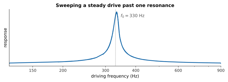
Figure 4.4:A steady drive of constant strength, swept slowly from 120 Hz to 900 Hz past a resonance at 330 Hz. The drive does not change in strength at any point. Everything you hear is the resonator’s selectivity.
What you hear: A tone gliding slowly upward. For most of the sweep it is barely audible; as it passes about 330 Hz it swells dramatically, then dies away again as the glide continues.
Listen: Resonance Sweep
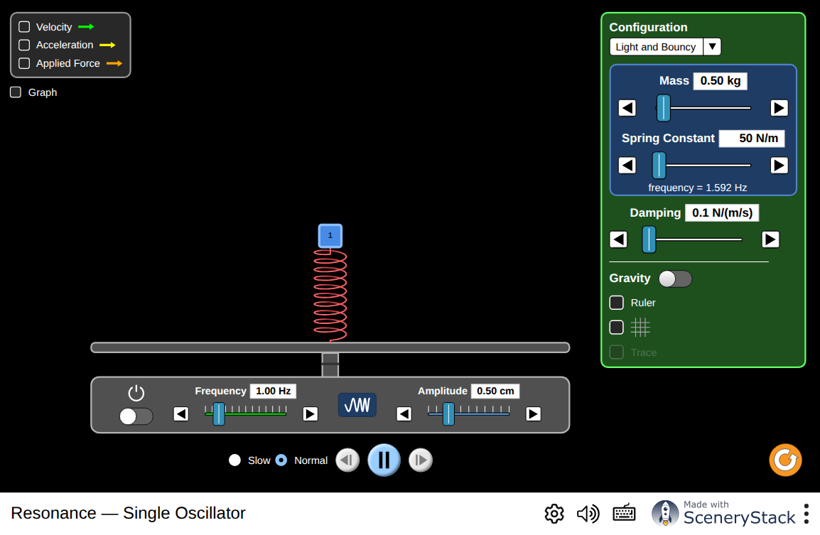
Figure 4.5:Set the damping low and sweep the driving frequency slowly through the natural frequency. The mass always moves at the driving frequency; it is the amplitude that changes, rising sharply at resonance. Increase the damping and repeat: the peak becomes lower and broader. Then change the mass or spring constant, predict which way the resonance will move, and test your prediction.
Interactive simulation: Resonance — single oscillator
Phase: Pushing at the Right Moment¶
Why does driving at work so well? The answer is about timing, and it is better than the usual “the pushes add up”.
To feed energy into an oscillator you must push in the direction it is already moving, push in phase with the velocity, not with the displacement. For a sinusoid, velocity leads displacement by a quarter cycle. So the drive must lead the displacement by , which is exactly the phase relationship the bottom panel of the figure shows at resonance.
Off resonance, the drive and the motion drift in and out of step, so some pushes add energy and others take it away, and the amplitude never builds. At resonance the relationship is locked, and every push helps.
This is also why a child on a swing must push at the right moment rather than merely often, and why pushing twice as often does not work at all.
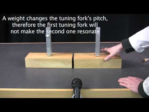
Figure 4.6:MIT’s Physics Instructional Resources Lab demonstrates natural frequency and sympathetic vibration with matched tuning forks. One resonator responds strongly because the other drives it at the frequency it already prefers.
Watch on YouTube: Tuning Forks
4.3Damping, Bandwidth, and the Quality Factor¶
Damping Sets the Height and the Width¶
What stops the amplitude at resonance from growing without limit is damping. Energy is fed in by the drive and lost to friction and radiation, and the amplitude settles where the two balance.
So a lightly damped system reaches a very large amplitude before it balances: a tall peak. It is also fussy: because it loses so little energy per cycle, it takes many cycles to build up, and during those cycles the drive must stay in step, which it will only do if the frequency is very close to . Tall and narrow go together.
A heavily damped system balances quickly at a modest amplitude and is not fussy, because it never needed many consecutive well-timed pushes. Short and broad go together.
Defining ¶
The quality factor measures this, and it can be defined in three equivalent ways:
where is the width of the response peak between the points at which the amplitude has fallen to of its maximum, and is the free-decay time of Chapter 1.
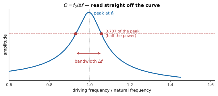
Figure 4.7:How is measured. Find the peak, drop to 0.707 of its height, which is half the power, since power goes as amplitude squared, and measure the width between the two crossings. The quality factor is the peak frequency divided by that width.
The third definition, , is the one that connects this chapter to the last. It says that a narrow resonance and a long ring are the same fact, measured two different ways. Something that takes a long time to stop is something that is fussy about what starts it.
The Shape of the Response Curve¶
summarizes the response curve with a single number, its ratio of peak frequency to width. The curve itself, amplitude against driving frequency, has a definite shape, and it is worth writing down, because it is what a real measurement produces and what the rest of the book quietly assumes.
Write the driving frequency as a ratio to the natural frequency, , so is exactly on resonance. The steady-state amplitude, relative to how far the same force would push the system if applied very slowly (), is
Three checks confirm this is the curve already described in words. Far below resonance (), both terms under the root vanish and : the mass simply follows the force, as §4.2 said. Exactly on resonance (), the first term vanishes and only the damping term survives, leaving : the peak height is nothing but itself, restated as a formula. Far above resonance (), the term dominates and the response falls as : the mass cannot keep up, and doubling the driving frequency above resonance cuts the response to a quarter.
Where the response formula comes from
The equation of motion for a mass on a spring with damping constant , driven by a force , is
After the initial transient dies away, the system settles into oscillating at the driving frequency, , for some amplitude and phase lag . Substituting this trial solution and collecting the sine and cosine parts separately gives two equations, which combine to
The static response, at , is just . Dividing the general expression by this, and writing everything in terms of and (which is equivalent to the definitions already given), reduces the ratio to the compact form quoted above. None of the algebra changes the physics already argued from the shape of the curve; it only makes the peak height, the low- and high-frequency limits, and the falloff exact rather than qualitative.
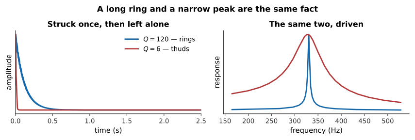
Figure 4.8:The same brief tap, through two resonators tuned to the same frequency and differing only in damping. The left panel of the figure shows what you hear; the right panel shows the response curves of the same two resonators when driven instead. A long ring and a narrow peak are two views of one property.
What you hear: Two struck sounds at the same pitch. The first rings on clearly for a second or more, like a struck glass; the second is a dull thud that is over almost at once.
The Instrument Maker’s Trade-off¶
Now the trade-off can be stated properly, and it is the central design tension in acoustic instruments.
Energy radiated as sound is energy lost from the vibration, and energy lost from the vibration lowers . So:
| High | Low | |
|---|---|---|
| Response | Huge, but only very near | Modest, over a wide band |
| Ring | Long | Short |
| Loudness | Quiet | Loud |
| Examples | Tuning fork, wine glass, bell | Guitar body, violin body, drum head |
A tuning fork has a of several thousand: it is a superb frequency standard and an almost useless loudspeaker, so it must be pressed against a table to be heard. A guitar body has a of around five: a poor frequency standard and an excellent radiator.
The requirement for a resonator in an instrument is therefore almost the opposite of the requirement for the vibrator. The string should have high , it holds the pitch and sustains the note. The body should have low , it should amplify everything the string offers, equally, and get it into the room. Chapter 10 shows how the bridge mediates between the two.
4.4Normal Modes¶
Two Masses, Two Modes¶
Move from one mass to two, coupled by a spring between them, and something new appears.
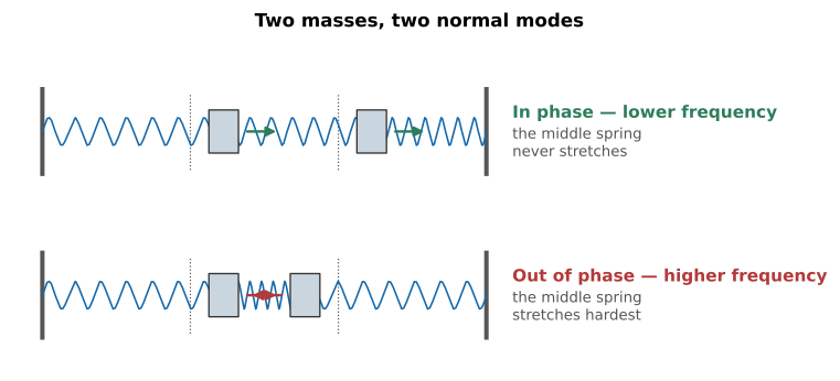
Figure 4.9:The two normal modes of a two-mass system. In the in-phase mode the masses move together and the connecting spring is never stretched, so it contributes no restoring force and the frequency is lower. In the out-of-phase mode they move oppositely, the connecting spring is stretched hardest, and the frequency is higher.
A normal mode is a pattern of motion in which every part of the system oscillates at the same frequency with a fixed relative amplitude and phase. Set a normal mode going and it persists, keeping its shape, exactly like a single mass on a single spring.
Two masses give two modes. The general rule is that a system with degrees of freedom has exactly normal modes, no more, and no fewer.
Start such a system in some arbitrary way, and it will not keep its shape: the motion looks complicated and never quite repeats. That is because you have excited both modes at once, and they are running at different frequencies.
Many Masses, Many Modes¶
Add masses and you add modes. A string is the limit of this process: infinitely many infinitesimal masses, and therefore infinitely many modes, which is exactly the family of standing waves Chapter 3 found.
The modes of a string are special in one respect, and the specialness is the reason music exists. Their frequencies are : exact whole-number multiples. Nothing guarantees this in general. The modes of a drumhead are in the ratios , and the modes of a bar are in the ratios : the reason Chapter 12 is a chapter about instruments with no definite pitch.
Any Motion Is a Sum of Modes¶
Here is the central result of the chapter.
Any motion of the system, however complicated, can be written as a sum of its normal modes, each with its own amplitude and phase. The modes form a complete set. Nothing the system can do lies outside them.
This transforms the problem of a plucked string from something apparently intractable, a triangle of string, released from rest, into bookkeeping. Decompose the initial shape into modes, let each mode oscillate at its own frequency, add them back up.
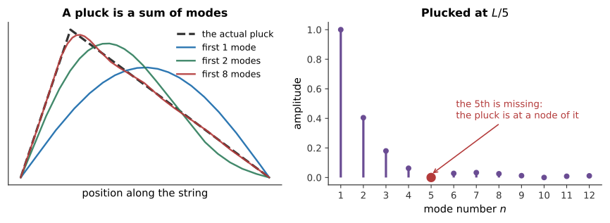
Figure 4.10:A string plucked one-fifth of the way along. Left: the triangular shape, rebuilt from its modes, one mode is a poor fit, eight are very nearly exact. Right: how much of each mode the pluck contains. The fifth mode is entirely absent, because the pluck point is a node of it: you cannot excite a mode by pulling on a place that mode does not move.
That missing fifth mode is not a curiosity; it is a technique. Guitarists pluck near the bridge for a bright sound and over the soundhole for a mellow one, and what they are doing is choosing which modes to leave out. Chapter 10 makes the rule explicit: plucking at silences the th harmonic and every multiple of it.
Finding the mode amplitudes: Fourier’s method in advance
Decomposing the pluck is a calculation, and Chapter 5 is about to do the same thing to sound.
The modes of a string fixed at both ends are . The claim is that any initial shape satisfying can be written
To find a particular , use the fact that the modes are orthogonal:
Multiply both sides of the expansion by and integrate over the string. Every term on the right vanishes except the one with , leaving
For a string plucked to a height at a point along its length, this integral evaluates to
Two things fall out immediately. The makes the high modes weak, so a plucked string is not harsh. And the vanishes whenever : the missing-mode rule, now derived rather than asserted.
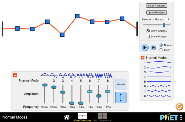
Figure 4.11:A chain of masses whose number you can change. Excite one mode at a time and watch it hold its shape; then excite two at once and watch the motion stop looking like anything in particular. Note that masses always give exactly modes.
Interactive simulation: Normal Modes
4.5Resonators in Musical Instruments¶
The Helmholtz Resonator¶
The simplest acoustic resonator is a cavity with a narrow opening: a bottle. Blow across the top and it sounds one note, and only one.
The mechanism is a mass on a spring, made entirely of air. The plug of air in the neck is the mass. The much larger body of air in the cavity is the spring: push the plug in and you compress the cavity, which pushes back. Its frequency is
where is the neck’s cross-sectional area, its effective length, and the cavity volume.
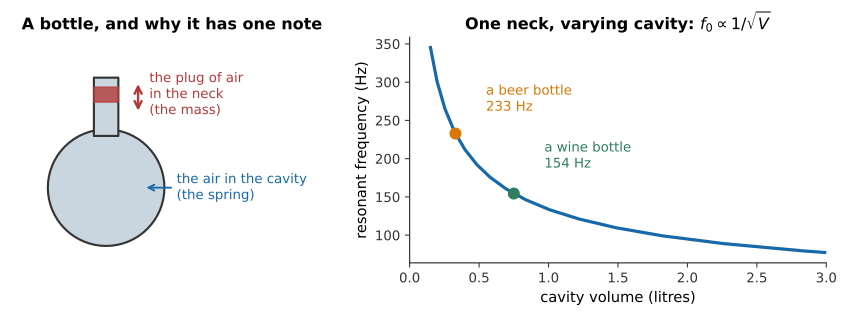
Figure 4.12:The Helmholtz resonator. Unlike a pipe, it has essentially one resonance, not a harmonic series, because there is no length along which standing waves can fit, only a single mass bouncing on a single spring. Filling the bottle with water reduces and raises the pitch, in inverse proportion to the square root of what is left.
A guitar body is a Helmholtz resonator whose neck is the soundhole, and its air resonance, around 100 Hz on a typical steel-string, is deliberately placed near the bottom of the instrument’s range, where the top plate alone radiates poorly. The same trick appears as a bass-reflex port in a loudspeaker cabinet (Chapter 15).
Bodies, Bores, and Cavities¶
Every acoustic instrument contains at least one resonator. The list below names which is which before Part V takes them one at a time.
| Instrument | The vibrator | The resonator |
|---|---|---|
| Guitar, violin, piano | The string | The body, the soundboard, and the air inside |
| Flute, clarinet, trumpet | The air jet, reed, or lips | The air column in the bore |
| Timpani | The membrane | The kettle of air beneath it |
| Voice | The vocal folds | The vocal tract |
The wind instruments are the odd family out, and the difference is fundamental. In a string instrument the resonator merely responds to the vibrator, which sets the pitch on its own. In a wind instrument the resonator controls the vibrator: the air column feeds back on the reed or the lips and tells them what frequency to oscillate at. That feedback is why a clarinetist can play a scale with one reed, and why Chapter 11 needs a different kind of argument from Chapter 10.
Resonance as Amplifier and as Filter¶
A final framing, which will be used repeatedly.
A resonator does not create energy. It is not an amplifier in the electrical sense, nothing is being added. What it does is provide a much better path for energy to leave the vibrator and enter the air, by presenting a large radiating surface where there was a thin string. The sound is louder and the note is shorter, and the total energy is unchanged.
A resonator is also a filter. It responds strongly to the frequencies near its peaks and weakly to the rest, so it reshapes the spectrum of whatever drives it. A guitar body’s dozens of resonances are collectively a fixed filter through which every note passes, and two guitars differ because their filters differ.
That view, a source with a spectrum, passed through a filter with a shape, is the single most useful model in the rest of this book. It is the model of the singing voice (Chapter 13), of the vowel, of subtractive synthesis (Chapter 15), and of why a violin sounds like a violin whatever note it plays.
4.6Summary¶
Free vibration happens at an object’s natural frequency; driven vibration happens at the driving frequency. What the natural frequency controls is not the frequency of the response but its size.
Resonance is the large response obtained by driving at a natural frequency. It works because at resonance the drive leads the displacement by exactly , in phase with the velocity, so every push adds energy.
The quality factor measures the sharpness of a resonance. A narrow peak and a long ring are the same fact stated two ways.
Loudness and sustain trade against each other, because radiating sound is a loss of energy and losses lower . Instruments therefore want a high- vibrator and a low- resonator: a tuning fork has in the thousands and is nearly silent, a guitar body has near five and is loud.
A normal mode is a pattern in which every part oscillates at one frequency with fixed relative amplitudes. A system with degrees of freedom has exactly of them; a continuous object has unlimited numbers.
Any motion is a sum of normal modes. A plucked string is decomposed into modes, each oscillates at its own frequency, and the sum is the motion. Plucking at excites no th mode, because the pluck point is a node of it.
A string’s modes are harmonic, exact whole-number ratios, but this is special. Bars and membranes are not, so percussion instruments mostly lack definite pitch.
A Helmholtz resonator is a plug of air on a spring of air, with a single resonance at . It is a bottle, a guitar’s air mode, and a loudspeaker’s bass port.
A resonator is both an amplifier and a filter: it speeds energy out into the air, and it reshapes the spectrum passing through it. Source-plus-filter is the model used for the rest of the book.
4.7Check Your Understanding¶
Five short, auto-graded questions cycle within one compact activity. The set mixes multiple response, true/false, drag-the-words, fill-in-the-blank, and mark-the-words formats.
Multiple response. Which changes lower the resonance frequency of a Helmholtz resonator? Select from: increase cavity volume; lengthen the effective neck; increase neck area; increase the speed of sound.
True or false. After transients die away, a driven oscillator vibrates at its natural frequency rather than at the driving frequency.
Drag the words. Complete: quality factor is resonance frequency divided by ___; a high- resonance has a ___ response peak and a ___ decay time. (Terms: bandwidth, narrow, long, wide, short.)
Fill in the blank. A system with two degrees of freedom has ___ normal modes.
Mark the words. Identify the two functions of a resonator in this sentence: “A resonator transfers energy efficiently to the air and filters the source spectrum; it does not create energy.”
4.8Conceptual Questions¶
A driven oscillator settles into oscillating at the driving frequency rather than its own. Explain what role its natural frequency then plays.
A child on a swing is pushed once per swing, and the swing grows. Explain why pushing twice per swing does not work, in terms of the phase of the drive relative to the velocity.
A tuning fork has a of several thousand and a guitar body a of about five. Which is louder, which rings longer, and explain why those two answers must go together.
Explain why a tall resonance peak is necessarily a narrow one, without using any formula.
Two masses connected by springs have two normal modes. Explain why the in-phase mode has the lower frequency.
A guitarist plucks a string exactly one-third of the way along. Which harmonics are missing from the resulting note, and why?
Explain why a bottle has essentially one resonance while an organ pipe has a whole harmonic series, even though both are containers of air.
In a violin, the string sets the pitch and the body responds. In a clarinet, the air column tells the reed what pitch to sound. Explain why this difference makes the two instruments require different kinds of analysis.
4.9Problems¶
Solution to Exercise 4.1 #
Solution to Exercise 4.2 #
(a) From :
(b) From :
(c) The singer must land within roughly a tenth of a hertz of 720 Hz, about a quarter of a cent, and hold it. That is far finer than any singer can aim deliberately, so the demonstration is usually done by sweeping slowly through the region until the glass responds, rather than by hitting the note directly.
Solution to Exercise 4.3 #
(a) Hz.
(b) Centered on 98 Hz, the half-power range runs from about Hz to Hz.
(c) In semitones:
Therefore, the resonance usefully covers about three semitones. A low is what makes even that possible; the wine glass of the previous problem covers about four thousandths of a semitone.
Solution to Exercise 4.4 #
(a) Converting to SI: m³, m², m.
(b) Halving the air volume, with the neck unchanged:
Therefore, the empty bottle sounds about 142 Hz and the half-full one about 201 Hz: a rise of cents, exactly a tritone. Halving the volume always raises the pitch by exactly this interval, whatever the bottle.
Solution to Exercise 4.5 #
(a) Plucking at puts the pluck point at a node of the 4th mode and of every multiple of 4. So harmonics 4, 8, 12, … are absent.
(b) Hz, Hz, Hz.
(c) At , which is a node of the 3rd mode (and of the 6th, 9th, …).
Therefore, the pluck position acts as a comb filter on the harmonic series, removing one harmonic and all its multiples, which is exactly the control a guitarist exercises by moving the right hand.
Solution to Exercise 4.6 #
The response is , with .
(a) : the first term vanishes, leaving
(b) :
(c) :
Therefore, the amplitude at resonance is times the static response, while an octave below it is only 1.3 times and an octave above it is one third: the resonator suppresses frequencies above its peak rather than merely failing to boost them.
Solution to Exercise 4.7 #
(a) With :
(b) As ,
Therefore, strong coupling splits the two mode frequencies widely apart, and weak coupling brings them together. In the limit of no coupling the two masses are independent oscillators of identical frequency: the “two modes” have become indistinguishable, which is what you would expect of two unconnected copies of the same thing.
Solution to Exercise 4.8 #
Solution to Exercise 4.9 #
Solution to Exercise 4.10 #
The number of cycles in one decay time is . From ,
The frequency has canceled: the number of cycles depends only on .
For the tuning fork,
Therefore, a fork of rings for about 1300 cycles before falling to . At 440 Hz that is about three seconds; at 256 Hz, about five. The lower fork rings longer in time while ringing the same number of cycles.
Solution to Exercise 4.11 #
(a) Using :
| Mode | Drumhead ratio | cents | String ratio | cents |
|---|---|---|---|---|
| 1 | 1.00 | 0 | 1 | 0 |
| 2 | 1.59 | 804 | 2 | 1200 |
| 3 | 2.14 | 1318 | 3 | 1902 |
| 4 | 2.30 | 1444 | 4 | 2400 |
| 5 | 2.65 | 1688 | 5 | 2786 |
(b) The string’s partials are exact whole-number multiples of one frequency, so they are all harmonics of a single fundamental, and the auditory system can assign one pitch to the whole set (Chapter 8). The drumhead’s are not multiples of anything: 1.59, 2.14, and 2.30 have no common fundamental, so there is no single frequency the set points to.
Therefore, the drumhead gives the ear a collection of unrelated frequencies rather than a harmonic series, and the ear reports a sound with a rough pitch region rather than a note.
Solution to Exercise 4.12 #
(a) Hz and Hz.
(b) Together they cover about 30 Hz out of a range of Hz, or about .
(c) Two resonances plainly cannot account for the instrument’s ability to radiate every note. The real body has dozens of modes above these, increasingly closely spaced, which merge into a broad and lumpy response rather than a set of isolated peaks. The two named resonances matter because they are isolated and therefore individually audible, they are the ones a maker can tune, but the rest of the range is radiated by a forest of overlapping higher modes.
Solution to Exercise 4.13 #
(a) The midpoint is a node of every even mode, so harmonics 2, 4, 6, 8, … are absent. Only odd harmonics remain.
(b) A midpoint pluck is the least bright pluck available. It removes every even harmonic outright, and the factor together with the falloff leaves the surviving odd harmonics weak as well. A pluck close to the bridge, at small , makes small for low and comparatively large for high , so the spectrum tilts toward the high harmonics and the note is bright and thin.
Therefore, the same string can be made mellow or brilliant by nothing more than the choice of pluck point: a guitarist’s right hand moves as much as the left for that reason.
Solution to Exercise 4.14 #
(a) The peak response at resonance is proportional to , so it rises by .
(b) The bandwidth is , so it falls by the same factor: to of what it was.
(c) The player would find that notes near the body resonance are louder and ring longer, while notes away from it are relatively weaker: the instrument has become less even across its range, and more colored. It would also sustain more and project less overall, since a higher means less energy is leaving as sound per cycle.
Therefore, the trade-off of §4.3 appears directly as a design decision: bracing for evenness and volume means accepting a shorter sustain, and bracing for sustain means accepting an uneven instrument.