Laboratory Exercises - Physics of Music

The claims this book makes about spectra, air columns, beats, and reverberation are all measurable, most of them in an afternoon, several of them with a telephone. This appendix is a set of ten exercises that take the book’s assertions and check them.

They are written to be run with whatever is available. Where a laboratory has an oscilloscope and a function generator, use them: reading a waveform off a calibrated screen builds an intuition that a software display does not. Where it does not, every exercise here has a software path, and that path is now a browser tab. The simulations named below open from a link, install nothing, ask for no account, and read the laptop’s own microphone; the only downloads this appendix still asks for are for the two exercises that need to edit a recording.

Equipment¶

The short list. A laptop, a pair of headphones, and a phone will do all ten exercises at reduced precision.

Item	Laboratory version	Substitute
Signal source	Function generator	The generator built into the Oscilloscope simulation: sine, square, triangle, sawtooth, pulse, and noise, with amplitude, `DC` offset, and duty cycle. It draws its output rather than playing it, so for a tone you have to hear, use the Composer screen of Wave Composer
Waveform display	Oscilloscope	The same Oscilloscope simulation, driven by its own generator or by the microphone: two channels, `AC`/`DC`/`GND` coupling, triggering, `X-Y` and `FFT` modes, $\Delta t$ and $\Delta V$ cursors, live frequency, period, $V_\text{pp}$ and $V_\text{rms}$ readouts, and `CSV` export
Spectrum analyzer	Dedicated analyzer, or a scope with `FFT`	The Oscilloscope’s `FFT` mode for one spectrum at a time; the Analyzer screen of Wave Composer for a live spectrogram with the instantaneous spectrum and an `LPC` envelope beside it. Audacity’s Analyze > Plot Spectrum or Sonic Visualiser if you would rather work from a saved file
Sound level meter	Calibrated Type 2 meter	Nothing in a browser substitutes for this one. A phone `SPL` app, uncalibrated, so use it for differences, never absolute levels
Microphone	Measurement microphone	The laptop’s built-in microphone, which both simulations read directly once you grant the browser permission
Miscellaneous	Meter rule, thermometer, tuning fork, a length of string, a set of masses, a pulley, a long tube or a graduated cylinder	A tape measure, an outdoor thermometer or the day’s weather report, a tuning-fork app, fishing line, kitchen scales and any objects you can hang from them, a smooth rod or a pencil taped to a table edge for the pulley, and a cardboard tube or a tall bottle for the air column. Where the apparatus is missing outright, What a Simulation Can and Cannot Replace says which exercise a simulation can carry instead

One warning about phone apps. A phone microphone rolls off sharply below about 100 Hz and its automatic gain control fights you. Turn off any noise-suppression or “voice enhancement” setting before recording, and never trust a phone for an absolute sound level. The same warning applies to a laptop microphone feeding a simulation: what you are measuring is the shape of a spectrum and the ratios of frequencies, never an absolute level.

What a Simulation Can and Cannot Replace¶

Three of the book’s simulations do most of the bench work. The Oscilloscope is a function generator and a dual-channel scope in one window; Wave Composer synthesizes tones and analyzes live or recorded sound; and Standing Waves and Resonance supply the apparatus of two exercises whose hardware is the hardest to improvise.

Where a simulation appears in the table below, it is genuinely the instrument, not a picture of one: you set the controls, read the numbers off the screen, and write them up the same way. Where the entry says rehearsal, the quantity the exercise asks for is an input to the model rather than an output of it, and running the simulation teaches you the procedure but cannot measure the world.

Exercise	Simulation	What it gives, and what it does not
B.1	Oscilloscope	The whole exercise. The generator is silent, so step 4’s what changes in what you hear needs a tone from Wave Composer or a real generator alongside
B.2	Standing Waves, Standing Waves screen	Rehearsal only. The speed of sound is what the model is given, not what it finds; the measurement needs a real tube and a real thermometer
B.3	Wave on a String	The harmonic sweep of step 2 and the shape of every mode. Tension is a slider without units, so the $f_1$ against $\sqrt{T}$ plot and the value of $\mu$ need the real apparatus
B.4	Resonance, Single Oscillator screen	The whole exercise, and better than the bench version: you set the mass, stiffness, and damping, so the $Q$ you measure from the bandwidth can be checked against the $Q$ those numbers predict
B.5	Wave Composer, Analyzer screen	Spectra and spectrograms of anything you play into the microphone, which is the body of the exercise. The listening test needs an editor to cut the attacks off
B.6	—	None. Levels, distances, and rooms are physical
B.7	Wave Composer, Composer screen	Steps 1 and 2: it sums up to four sinusoids and beat pairs and plays them, so the beats are both visible and countable. Steps 3 and 4 measure you, and need a partner
B.8	Wave Composer, Analyzer screen	The frequency measurement, by pitch tracking over roughly 60 to 800 Hz, which covers the middle octave step 2 asks for. The instrument itself has to be real
B.9	Standing Waves, Instruments screen	The prediction, exactly: the 1 : 2 : 3 and 1 : 3 : 5 ratios and the stopped pipe’s octave drop. It deliberately omits the end correction, which is the quantity this exercise measures, so the discrepancy between it and your tube is the result
B.10	—	None. Two real rooms, or nothing

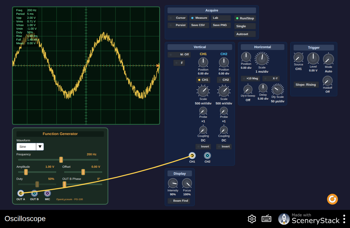
A phosphor-green oscilloscope graticule beside vertical, horizontal, and trigger controls, with a function generator patched to channel one. — Figure 1:The bench of B.1, and of most of what follows. Its *Lab* menu holds four short drills, measuring $V_\text{pp}$ , catching a normal trigger, finding the third harmonic in `FFT` mode, and matching a 90° Lissajous figure, which between them cover every control the exercises use. Work through those before touching a real instrument, and the real instrument stops being intimidating.
Interactive simulation: Oscilloscope

How to Write These Up¶

Each exercise ends with an analysis section. A complete write-up has four parts, and the third is the one most often skipped:

What you measured: the raw numbers, with units, in a table.
What you calculated: the derived quantity, with the formula used.
How well it agrees: the percentage difference from the prediction, and an estimate of your own uncertainty. “Within 3%” means nothing until you say whether your measurement was good to 1% or to 10%.
What the discrepancy means, either the prediction is confirmed within uncertainty, or something is unaccounted for. Say which, and if the latter, name a candidate.

B.1 The Oscilloscope and the Function Generator¶

Supports Chapters 1–2. Time 60–90 minutes. Simulation Oscilloscope.

The point of the first exercise is not to discover anything. It is to learn to read the two instruments the rest of the exercises depend on, and to connect what you see on a screen to what you hear.

Procedure¶

Set the function generator to a 440 Hz sine wave and display it on the oscilloscope. Adjust the time base until two or three full cycles fill the screen.
Measure the period directly from the screen. Calculate the frequency and compare with the generator’s setting.
Double the frequency to 880 Hz. Predict what happens to the trace before you press the button, then check.
Return to 440 Hz and halve the amplitude. Record what changes on the screen and what changes in what you hear.
Switch the generator to square, triangle, and sawtooth at the same 440 Hz. Sketch each waveform and describe in one sentence how each sounds compared with the sine.
Sing or play a sustained note into a microphone and display it. Identify the period on the screen and calculate the frequency.

Analysis¶

From your measured period in step 2, what is your frequency and its uncertainty? Which is the limiting factor: the resolution of the time base, or your ability to judge where a cycle begins?
Rank the four waveforms of step 5 from dullest to brightest. Chapter 5 will explain the ranking; record the order now, before you know the answer.
The trace in step 6 is not a clean sinusoid. List two things visible in it that are not visible in the generator’s sine.

B.2 The Speed of Sound¶

Supports Chapter 2. Time 60 minutes. Simulation Standing Waves, for rehearsal only.

Method A, Resonance in a tube¶

Hold a vibrating tuning fork of known frequency $f$ over the open end of a tube whose length can be varied (a graduated cylinder being filled with water works well).
Find the shortest length $L_1$ at which the tube resonates loudly, and then the next length $L_2$ .
The distance $L_2 - L_1$ is half a wavelength. Calculate $\lambda$ and then $v = f\lambda$ .

Using the difference of two resonance lengths rather than the first length alone eliminates the end correction, which is exactly what you want here and exactly what you will measure in B.9.

Method B, Time of flight¶

Place two microphones several meters apart, as far apart as your interface allows, and record both to the same file.
Make a sharp impulsive sound (a hand clap, two blocks struck together) beyond one microphone, on the line joining them.
Measure the delay between the two arrivals in the recording, and divide the separation by it.

Analysis¶

Record the air temperature. Calculate the predicted speed of sound and compare.
Which method gave the smaller uncertainty, and why?
Method B is sensitive to where you stand. Explain why standing off the line joining the microphones makes the measured speed come out too high.

B.3 Standing Waves on a String¶

Supports Chapter 3. Time 90 minutes. Simulation Wave on a String, in part.

Procedure¶

Stretch a string horizontally from a mechanical vibrator over a pulley to a hanging mass, so that the tension is $T = mg$ and the vibrating length $L$ is between the vibrator and the pulley.
Drive the string and sweep the frequency slowly upward from a few hertz. Record every frequency at which a clean standing-wave pattern appears, and the number of loops in each.
Repeat for at least four different hanging masses.
If a second string of different thickness is available, repeat step 2 for it at one fixed tension.

Analysis¶

For one tension, plot $f_n$ against $n$ . The points should lie on a straight line through the origin. Do they? What is the slope, and what does it mean?
Plot $f_1$ against $\sqrt{T}$ for your four masses. Is it linear? Extract the linear mass density $\mu$ from the slope and compare with the value you get by weighing a measured length of the string.
The frequency at which a pattern looks best is not sharply defined. Estimate the width of the frequency range over which each resonance is visible, and use it to put an uncertainty on $f_n$ .

B.4 Resonance and the Quality Factor¶

Supports Chapter 4. Time 60 minutes. Simulation Resonance.

Procedure¶

Choose a resonator: a wine glass, a length of pipe, a guitar body, or the string apparatus of B.3 held at one mode.
Drive it with a loudspeaker fed from the function generator, and measure the response amplitude with a microphone as you step the frequency through the resonance in small increments.
Take at least fifteen points, closely spaced near the peak.
Separately, excite the resonator impulsively (tap it) and record the decay.

Analysis¶

Plot amplitude against frequency. Find the peak frequency $f_0$ , and the two frequencies either side at which the amplitude has fallen to $1/\sqrt{2}$ of the peak. The difference between them is the bandwidth $\Delta f$ ; calculate $Q = f_0/\Delta f$ .
From your impulse recording, measure the time for the amplitude to fall to $1/e$ of its initial value. Estimate $Q$ from the decay and compare with the value from the response curve.
A wine glass has a $Q$ in the hundreds; a guitar body’s main resonance has a $Q$ of order ten. Explain, in terms of the instrument’s job, why a guitar should not have a high- $Q$ body.

B.5 The Spectra of Musical Instruments¶

Supports Chapter 5. Time 90 minutes. Simulation Wave Composer.

This is the central exercise of the course.

Procedure¶

Record the same pitch, A3 at 220 Hz is convenient, played by at least four sources: a sung vowel, a plucked string, a bowed or blown sustained tone, and a pure sine from the generator. Record several seconds of steady tone from each, at roughly equal loudness.
For each recording, select a window from the middle of the sustained portion, well clear of the attack, and compute its spectrum.
Record the frequency and relative amplitude of the first eight partials of each.
Now record just the first half-second of each note, including the attack, and make a spectrogram of it.

Analysis¶

Tabulate the partial amplitudes, in dB relative to the strongest partial, for all four sources. Which instrument has the strongest high harmonics? Does the ranking match the brightness you hear?
Are the measured partial frequencies exact integer multiples of the fundamental? Report the deviation of the eighth partial as a percentage. Which source is least harmonic, and why might that be?
From the spectrograms: describe how each note’s spectrum changes during the first tenth of a second. Which partials arrive first?
The listening test. Using an audio editor, cut the attack off each recording and play only the steady portions to a listener who has not seen which is which. How well can they identify the instruments? Relate the result to §5.4.

B.6 Sound Level, Distance, and Addition¶

Supports Chapter 7. Time 60 minutes. Simulation none; this one is physical.

Use a sound level meter if one is available. A phone app will do, provided every conclusion is drawn from differences between readings.

Procedure¶

Outdoors, or in the largest and least reverberant space available, set up a loudspeaker playing steady pink noise.
Measure the level at 1, 2, 4, and 8 meters on the axis of the speaker.
Return to a fixed distance. Measure the level with one speaker, then with two identical speakers side by side playing the same noise file, then with two playing different noise files.
Measure the level of several ordinary sounds: a quiet room, conversation at a meter, a hand clap, traffic.

Analysis¶

Plot level against $\log_{10}(\text{distance})$ . The slope should be $-20\ \text{dB}$ per decade: that is, -6 dB per doubling. What slope did you get? If it is shallower, what does that tell you about the room?
In step 3, two speakers playing different noise should add to about +3 dB. What did two playing the same file give, and why is it different?
Using the equal-loudness contours of §7.4, estimate the loudness level in phons of your measured traffic noise, and say what you had to assume about its spectrum to do so.

B.7 Beats and the Just-Noticeable Difference¶

Supports Chapter 8. Time 45 minutes. Simulation Wave Composer, for steps 1 and 2.

Procedure¶

Sound two tones together: one fixed at 440 Hz, one variable. Sum them electrically if you can, or use two speakers.
Set the second tone to 441, 443, 446, 450, 460, and 480 Hz in turn. For each, record: the beat rate you count, and a one-word description of the sensation (beating, rough, two separate tones).
Now find your own frequency discrimination. Have a partner alternate between 440 Hz and a slightly different frequency, and narrow the difference until you can no longer reliably tell which is which.
Repeat step 3 at 220 Hz and at 3520 Hz.

Analysis¶

Plot your counted beat rate against the frequency difference. The prediction is a straight line of slope 1. Up to what difference does it hold, and what happens beyond?
At what frequency difference did beating give way to roughness, and roughness to two separate tones? Compare the second of these with the critical bandwidth at 440 Hz quoted in §7.5.
Express your discrimination threshold from steps 3 and 4 as a percentage of the center frequency at each of the three frequencies. Is the percentage constant? What does that tell you?

B.8 Measuring a Tuning¶

Supports Chapter 9. Time 90 minutes. Simulation Wave Composer, as the frequency meter.

Procedure¶

Choose a fixed-pitch instrument: a piano, an electronic keyboard, or a fretted guitar.
Record every note of one chromatic octave in the middle of its range, and measure the fundamental frequency of each to the nearest 0.1 Hz.
Also record notes two or three octaves apart, near the extremes of the instrument’s range.
If a second instrument of a different kind is available, repeat.

Analysis¶

Convert each measured frequency to cents above the lowest note of your octave. Tabulate alongside the equal-tempered values (0, 100, 200, …).
Plot the deviation in cents from equal temperament for each note. Is the instrument equally tempered within your measurement uncertainty?
Compare your measured major third and perfect fifth with both the just ratios (5:4 and 3:2) and the equal-tempered values. Which is the instrument closer to?
From step 3: is the instrument’s octave exactly 1200 cents? If you measured a piano, it very likely is not. Explain the result using §10.6.

B.9 Air Columns and the End Correction¶

Supports Chapter 11. Time 60 minutes. Simulation Standing Waves, for the prediction.

Procedure¶

Take a tube open at both ends. Measure its length and inside diameter.
Excite it, by blowing across one end, or with a loudspeaker at one end, and measure the frequencies of its first three resonances.
Close one end and repeat.
Repeat the whole procedure for a tube of noticeably different diameter but similar length.

Analysis¶

For the open tube, are the resonances in the ratio 1: 2: 3? For the stopped tube, are they in the ratio 1: 3: 5? Report the measured ratios.
Using the speed of sound at your measured temperature, calculate the effective length of each tube from its fundamental. Subtract the physical length to get the end correction.
Divide your end correction by the tube radius. Compare with the theoretical value of about $0.6r$ per open end quoted in §11.2. Does the second tube give a consistent answer?
A stopped tube of the same length sounds roughly an octave lower. Verify this from your measurements, and state the discrepancy.

B.10 Reverberation Time¶

Supports Chapter 14. Time 60 minutes, plus access to two very different rooms. Simulation none; this one needs two real rooms.

Procedure¶

Choose two rooms of markedly different character: a stairwell and a carpeted office, say. Measure the dimensions of each and estimate its volume.
In each, make a loud impulsive sound (a balloon burst is the classic; two hardwood blocks work) and record it.
From the recording, plot the decay of level in dB against time.
Repeat the measurement at three different positions in each room.

Analysis¶

Measure $T_{60}$ , the time for a 60 dB decay, by fitting a straight line to the decay curve. In most rooms you will not get a clean 60 dB above the noise floor; fit over the first 20 or 30 dB and extrapolate, and say that you did.
Use the Sabine equation with your measured $T_{60}$ and volume to find each room’s total absorption, and then its average absorption coefficient. Is the value plausible for the surfaces you can see?
Filter the recordings into octave bands and measure $T_{60}$ in each. Is the reverberation time the same at 125 Hz as at 4 kHz? What does the difference say about the room’s furnishings?
How much did your three positions disagree? Is the reverberant field as uniform as the Sabine model assumes?