Experiment 14 — A Cosmic-Ray Muon Telescope¶
Objectives¶
By the end of this experiment you should be able to:
Build and validate a coincidence detector, and distinguish true coincidences from accidentals.
Estimate a vertical muon intensity only if detector efficiency and non-muon coincidences can be independently constrained.
Compare corrected angular rates with a finite-acceptance model when the counts support a fit.
Calculate survival for a stated muon energy and production altitude, while distinguishing that model from what a one-altitude rate measures.
Textbook connection¶
Read §14.1–14.4, and §2.5 on time dilation. The muon is a second-generation charged lepton with the same electric charge and spin as the electron. Its discovery prompted the question “Who ordered that?”, attributed to I. I. Rabi. It is also an accessible relativistic particle in existence. Muons from upper-atmosphere showers can reach sea level because their laboratory-frame lifetimes are dilated.
This experiment closes the course by using the relativity of Weeks 1–3 to explain the particle physics of Chapter 14, with a detector you build.
Theory¶
Where muons come from¶
Primary cosmic rays — mostly protons and other nuclei — strike nuclei in the upper atmosphere and produce showers containing pions. Charged pions decay,
and many resulting muons penetrate the remaining atmosphere. They are charged and ionize matter, but their much larger mass than the electron’s greatly reduces radiative energy loss at a few GeV. A typical sea-level muon has energy around ; the muon’s rest energy is , so a typical Lorentz factor is of order , and lower-energy muons at are abundant.
Why they should not get here¶
The muon’s proper mean lifetime is . The length scale is
but it is not a distance traveled in the muon’s rest frame. For a hypothetical muon produced above the detector, a calculation that omits time dilation and sets gives lifetimes and a survival probability of
This is a model comparison, not a prediction of the observed flux: production occurs over a range of altitudes and energies. The familiar roughly one muon per square centimeter per minute is a flux integrated over arrival directions, not an intensity per steradian.
Why they do¶
In the laboratory frame the muon’s lifetime is dilated to , so its mean decay length at fixed speed is . For this is approximately , and survival from the assumed becomes — a factor of about larger.
In the muon’s frame the distance between the chosen production and detection events is in this constant-speed model. It crosses in about , close to one proper mean lifetime. The two descriptions are the same physics in different coordinates, and being able to give both is one of the things this course is for.
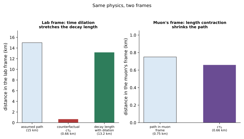
Figure 14.1:The same illustrative 15 km path in two frames, for and approximately constant speed. The bars compare mean decay lengths with distance; they do not represent measured production heights or energies.
The angular distribution¶
Muons arriving from a zenith angle must traverse a longer slant path through the atmosphere, roughly , and so are more likely to decay or be absorbed. For a restricted zenith and energy range, a useful empirical approximation is
with representative near-vertical intensity of order at sea level. The normalization and exponent depend on energy threshold, altitude, and angular range; the approximation is not reliable near the horizon. The central bench result is a validated coincidence rate. An exponent needs much longer runs.
Coincidence and accidentals¶
A single GM tube counts local radioactivity and electronic noise as well as muons. Requiring two aligned tubes to fire within a short window selects penetrating-particle candidates. Some correlated shower secondaries can also fire both, so coincidence alone does not identify every event as a muon.
For a symmetric timestamp cut , the rate of accidental coincidences from two independent stationary singles streams of rates and is approximately
For and this is , or about one event in 23 days. A short laboratory run cannot measure that tiny rate directly. Use the measured singles rates, an offset-timestamp control, and a timing-window scan to test the estimate and report an upper limit if no accidentals appear.
Geometric acceptance¶
For two ideal parallel planar detectors of area separated by , the solid angle subtended is approximately , and the near-vertical coincidence rate is
For , , and , and the ideal rate is only before efficiency losses. A 30-minute run then expects about 15 ideal counts, or 26% counting uncertainty. The finite geometry needs an acceptance calculation, and cylindrical GM tubes cannot simply use their external cross section as .
Pre-lab¶
Apparatus¶
Two larger-area GM tubes with matched high voltage and accessible pulse outputs, mounted rigidly one above the other with adjustable separation
Microcontroller coincidence unit with manufacturer-approved, isolated low-voltage pulse outputs and characterized timing inputs. Never connect a raw GM high-voltage pulse to a GPIO pin.
Rotating mount with an angle scale, or a rigid frame that can be set at measured zenith angles
Optional absorber placed between tubes for a penetration control
A data logger able to record long runs under the institution’s unattended equipment procedure
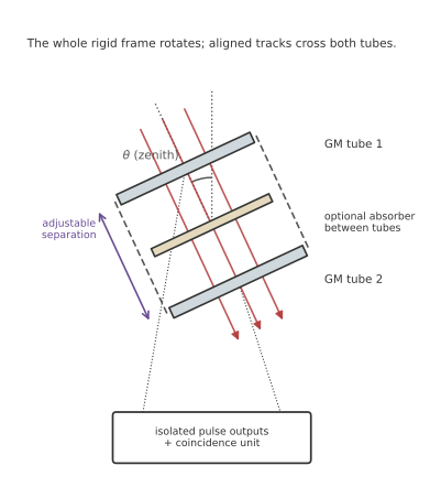
Figure 14.2:The two-tube coincidence telescope. Charged particles traversing both active volumes can trigger a count; the optional absorber tests penetration. Rotate the complete rigid frame to set its zenith angle .
Procedure¶
Before you build the telescope¶
Match the stacked-tube geometry, angle definition, adjustable separation, and coincidence electronics to Figure 14.2. Determine the active dimensions, projected shape, and center-to-center separation on the real instrument; the drawing is not to scale.
Label the tubes and electronic channels permanently. Record plateau voltage, threshold, pulse polarity, pulse width, cable length, and firmware version for each channel before combining them.
Check timestamp resolution, dropped pulses, and clock stability. Choose run names recording angle, separation, coincidence window, and start time; write metadata even for controls.
Level the rotation axis, define with a plumb line or inclinometer, and mark the tube centers. At each angle confirm that the two active areas remain aligned rather than merely reading the scale.
Make a run plan: singles, displaced-geometry control, timestamp-offset control, window scan, and a vertical baseline. Add angles only after a short rate test shows that they can accumulate useful counts.
Part A — Build and validate the coincidence unit¶
Set both tubes to their plateau operating voltages, individually, as in Relativistic Electrons from Beta Decay.
Configure the approved unit to timestamp pulses on both channels and count a pair when . Save both singles streams, pair time differences, and live duration, or save enough data to reconstruct them. Prevent one pair from being counted twice.
Record the singles rate of each tube separately, over at least 10 minutes.
[ ] Checkpoint 1. Show the instructor your singles rates and one minute of coincidence output.
Part B — Prove that the coincidences are real¶
Three controls test different failure modes:
Displace the tubes so their direct overlap is removed while the electronics and environment stay fixed. Record the residual coincidence rate or its Poisson upper limit; correlated shower particles may remain.
Offset one timestamp stream by much more than the timing window, wrapping within a long run if needed. Count offset matches at many shifts and compare their average with the independent-singles prediction.
Scan the symmetric half-window across the measured pair-time peak. Choose a width that contains the stable prompt peak while limiting accidentals. The prompt efficiency need not be flat below the timing jitter. Plot counts versus window width with Poisson intervals.
[ ] Checkpoint 2. Present the controls and chosen window before starting long runs. If the rate is too low to measure a control directly, show its upper limit and the corresponding live time.
Part C — The angular distribution¶
With the telescope vertical (), make a baseline run and estimate the live time needed for the planned uncertainty. At the illustrative ideal rate, 30 minutes gives only about 15 counts.
If time permits, rotate the whole frame to , , and ; give each angle enough exposure to provide a useful count or Poisson upper limit. Record actual live time and angle. Treat as an extension: rates are very low and the simple model may fail there.
Return to for a second baseline of comparable precision if possible. A rate difference may signal drift or changing environmental conditions and needs investigation.
Determine the active-area geometry and separation. For an absolute intensity, use an independently calibrated muon reference detector or a suitable third-detector efficiency measurement, and estimate correlated non-muon coincidences. A gamma check source or an unqualified tube data-sheet value does not give muon efficiency. Otherwise report the background-corrected coincidence rate and relative angular trend.
Part D (optional) — Penetration control¶
With the frame vertical, place the approved absorber between the tubes and compare the coincidence rate with a no-absorber run of comparable duration. Keep geometry fixed and include accidental and background intervals.
A modest absorber may suppress soft charged secondaries while transmitting most GeV muons. It does not measure a muon momentum spectrum or identify every surviving coincidence as a muon.
Analysis¶
Flux¶
For the narrow-angle, ideal planar approximation, a vertical measurement would give
where is a separately estimated correlated non-muon coincidence rate. With only two GM tubes, and are not determined by the singles and coincidence rates. Report an absolute intensity only when those quantities have independent support. The planar formula also needs a finite-geometry check.
For two planar rectangles of active width , height , and separation , this Monte Carlo estimates a vertical geometric factor for a direction-independent intensity:
import numpy as np
rng = np.random.default_rng(0)

n = 2_000_000
wx, wy, d = ..., ..., ...              # measured active dimensions, cm
A = wx * wy
x0 = rng.uniform(-wx/2, wx/2, n)
y0 = rng.uniform(-wy/2, wy/2, n)
u = rng.random(n)                       # cos(angle to telescope axis)
phi = rng.uniform(0, 2*np.pi, n)
shift = d * np.sqrt(1-u*u) / u
hit = ((np.abs(x0 + shift*np.cos(phi)) <= wx/2) &
       (np.abs(y0 + shift*np.sin(phi)) <= wy/2))
G0 = 2*np.pi*A*np.mean(u*hit)           # cm^2 sr
G_vertical_cos2 = 2*np.pi*A*np.mean(u**3*hit)  # for I ~ cos^2(zenith)
sG0 = 2*np.pi*A*np.std(u*hit, ddof=1)/np.sqrt(n)
sG_vertical_cos2 = 2*np.pi*A*np.std(u**3*hit, ddof=1)/np.sqrt(n)
The factor is the projected-area factor. The sampled directions are uniform in solid angle, with uniform from 0 to 1; sampling would instead bake a intensity into the sample. Report both geometric factors and their Monte Carlo uncertainties; compare with . The weighting changes the vertical count prediction for a finite field of view. For a real cylindrical GM tube, use its active volume and directional efficiency in a refined model. The difference between approximate and refined acceptances is a correction, not automatically an uncertainty.
If qualified, compare your vertical intensity with a reference for the same energy threshold and altitude; do not compare it with the all-direction flux of about .
The angular exponent¶
Fit raw counts with a Poisson model using each angle’s live time. For a narrow telescope, model its corrected rate as . For a broad acceptance, integrate over all directions that can cross both detectors after the entire frame rotates; is the track’s zenith angle, which differs from the frame angle for off-axis tracks. The telescope’s local geometric factor remains fixed when the whole rigid frame rotates, but the sky intensity across its field of view does not. Quote only if several angles have enough counts to constrain it; otherwise show intervals or upper limits and state the angular trend.
Time dilation¶
The one-altitude coincidence rate cannot determine a Lorentz factor or a survival fraction because the production rate, height distribution, and energy spectrum are unmeasured. As a model exercise, suppose a muon starts at with constant speed and ask what gives a specified survival probability :
For , convert this to using , then compare with a muon of total energy. This is a conditional threshold from chosen assumptions, not a lower bound extracted from your telescope data.
Post-lab questions¶
Going further¶
Two-altitude measurement. With a sufficiently large, calibrated telescope, compare rates at widely separated heights while matching zenith acceptance and energy threshold. Model additional atmospheric production and energy loss before interpreting the ratio as survival. A 100 m height difference changes the survival factor of a muon by only about 0.4%, before these other effects.
Penetration study. Compare well-measured rates with and without an absorber between the detectors. A modest thickness can help identify a soft component, but it does not yield a GeV muon momentum spectrum.
Stopped-muon lifetime project. Use a separate detector with a stopping target, fast scintillation readout, and a decay-electron trigger. Measure timing response and accidental delayed pairs before fitting a lifetime. A GM tube’s recovery time and this two-tube layout cannot reliably resolve a 2.2 stopped-muon decay.