Tunneling by Frustrated Total Internal Reflection

Experiment 8 — Tunneling by Frustrated Total Internal Reflection¶

Objectives¶

By the end of this experiment you should be able to:

Explain the mathematical correspondence between an evanescent electromagnetic wave and a quantum wavefunction inside a classically forbidden region.
Measure the transmission through a variable air gap and extract the decay constant $\kappa$ .
Evaluate the exact rectangular-barrier transmission formula numerically and compare it with its thick-barrier approximation.
Explain why tunneling probability is exponentially sensitive to barrier width, and what that implies for scanning tunneling microscopy and alpha decay.

Textbook connection¶

Read §8.4–8.7, on the rectangular barrier and tunneling. The correspondence exploited here is the same form of differential equation within the barrier: for one polarization component in the air gap and the stationary quantum wavefunction in a rectangular barrier, both equations have the form

\frac{d^2\psi}{dz^2} = \kappa^2\psi ,

(8.1)

with a real $\kappa$ and hence exponentially decaying — not oscillating — solutions. Boundary conditions and transmitted quantities must still be handled separately in the two systems.

Theory¶

The evanescent wave¶

Light inside glass of index $n$ striking a glass–air interface at an angle $\theta$ greater than the critical angle $\theta_c = \arcsin(1/n)$ is totally internally reflected. But the field does not stop at the interface: it continues into the air as an evanescent wave whose amplitude decays as $e^{-\kappa z}$ with

\kappa = \frac{2\pi}{\lambda}\sqrt{n^2\sin^2\theta - 1} .

(8.2)

For $n = 1.52$ at $\theta = 45°$ and $\lambda = 650\ \text{nm}$ , $1/\kappa$ is about $263\ \text{nm}$ , while the corresponding intensity decay length is about $131\ \text{nm}$ . The evanescent amplitude is small, but never exactly zero at a finite distance.

Frustrating it¶

Bring a second piece of glass close to the first. If the gap $d$ is comparable to $1/\kappa$ , the evanescent field still has appreciable amplitude when it reaches the second surface, where it can couple back into a propagating wave. Light appears on the far side of a gap that ray optics alone cannot describe. In the thick-gap tail, after correcting for incident illumination and camera dark signal, transmitted intensity has the form

I(d) = I_0\, e^{-2\kappa d} + I_{\text{stray}} ,

(8.3)

the factor of 2 appearing because intensity is proportional to squared field amplitude. $I_0$ here is an extrapolated tail amplitude, not the measured zero-gap intensity. The exact glass–air–glass transmission saturates toward unity as $d\to0$ for matched, uncoated glass; it is not a single exponential over the whole contact image. Fresnel coupling depends on polarization and angle. Fit a region where the measured log-intensity is approximately linear in $d$ , and report its range.

The quantum barrier¶

A particle of energy $E$ incident on a rectangular barrier of height $V_0 > E$ and width $L$ has a wavefunction that is a combination of growing and decaying exponentials inside the finite barrier. Their scale is set by

\kappa_q = \frac{\sqrt{2m(V_0 - E)}}{\hbar} ,

(8.4)

and the exact transmission coefficient for equal potentials on either side is

T_{\rm exact}=\left[1+\frac{V_0^2\sinh^2(\kappa_q L)} {4E(V_0-E)}\right]^{-1} .

(8.5)

For $\kappa_q L \gg 1$ , this approaches

T \approx \frac{16E(V_0 - E)}{V_0^2}\, e^{-2\kappa_q L} .

(8.6)

Compare (8.2) with (8.4) and the large-width dependence in (8.3) with (8.6). Gap and barrier width play corresponding roles, but their decay constants have different physical inputs and the interface factors differ.

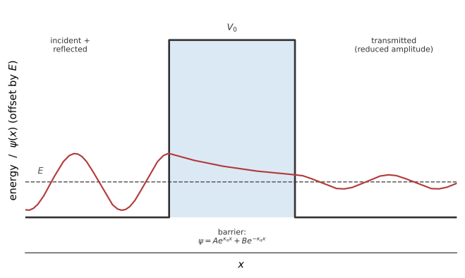
A potential barrier taller than particle energy, with a schematic oscillatory incident region, a nonoscillatory evanescent region, and a smaller transmitted oscillation. — Figure 8.1:The quantum side of the correspondence. The drawing is schematic; a finite barrier’s exact interior solution contains both exponential terms and must match the waves at both interfaces.

The Newton’s-rings trick¶

Controlling a sub-micrometre gap mechanically is difficult. Instead, use geometry: press a plano-convex lens of radius of curvature $R$ against the prism face. The gap between them at radial distance $r$ from the contact point is

d(r) = \frac{r^{2}}{2R} ,

(8.7)

so a single image of the contact region contains a continuous, calculable range of gaps. For $R = 1000\ \text{mm}$ , $d = 500\ \text{nm}$ at $r = 1.0\ \text{mm}$ — a comfortable field of view for a USB microscope.

A photograph can sample many gap widths without moving the lens, provided the incident beam illuminates that region uniformly or a spatial reference image corrects it. With a separate, near-normal reflected-light view, Newton’s rings can calibrate $R$ ; the ring relation assumes an approximately spherical surface, an air film, and one reflection phase reversal. Do not use the oblique total-internal-reflection image as a Newton’s-rings calibration.

Pre-lab¶

Apparatus¶

Right-angle prism, $n \approx 1.52$ , faces clean
Plano-convex lens with radius of curvature $R \approx 500$ – $2000\ \text{mm}$ , with $R$ known or measurable; specify the surface radius rather than assuming a focal length determines it without the glass index
Adjustable clamp or spring mount to press the lens against the hypotenuse face, with a fine adjustment
Diode laser, $650\ \text{nm}$ , with beam expander
Camera imaging the transmitted contact region, with calibrated position scale and linear response; alternatively a photodiode behind a pinhole on a calibrated translation stage. Provide a near-normal reflected-light view for Newton’s rings and a way to assess illumination uniformity.
Neutral-density filters and cleaning materials approved for the optics

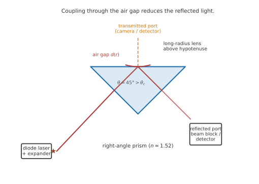
An expanded beam enters one short face of a right-angle prism, strikes its horizontal hypotenuse at an angle above critical, and exits the other short face after reflection; a lens above the hypotenuse receives light coupled through the thin air gap. — Figure 8.2:Frustrated total internal reflection. The lens approaches the prism’s **hypotenuse** from above. The curved air gap $d(r)$ permits transmission near contact and reduces the reflected intensity there. The drawing shows the ports, not the camera’s imaging optics or a scale drawing of the gap.

Procedure¶

Setup and controls¶

Identify the incident, reflected, and tunneled ports in Figure 8.2. Place a labeled detector or beam block at every port before switching on the laser.
Clean the prism hypotenuse and lens with approved lens tissue. Inspect both under room light; dust creates bright transmission spots that can look like tunneling and can scratch the surfaces when pressure is applied.
Mount the lens so it approaches normal to the hypotenuse and cannot slide. Mark the clamp position or record the force setting so contact pressure can be reproduced; never tighten beyond the apparatus limit.
Lock camera focus, aperture, and gain. Prepare an exposure log with pressure setting, exposure time, dark-frame name, image name, and saturation note.
Expand the beam enough to illuminate the planned fit region. Check its spatial uniformity or record a mapped reference image to correct a gradient; monitor incident power for drift. Establish pixel scale in the contact plane with a stage micrometer. Record the transmitted-port stray level with the lens well away, without moving the detector.

Part A — Establishing total internal reflection¶

Send the expanded beam through one short prism face so that it strikes the hypotenuse at $45°$ inside the glass. Verify the angle and measure or obtain the prism’s index at the laser wavelength. With the lens far away, confirm a bright reflected port and only stray light at the transmitted port.
Measure the residual transmitted intensity with nothing in contact. This is $I_{\text{stray}}$ and it sets the floor of your dynamic range. Reduce it — baffles and beam blocks — because the decay range is limited by the floor.

[ ] Checkpoint 1. Show the instructor the reflected and transmitted powers, and your measured stray floor relative to the brightest unsaturated transmitted signal you expect to measure. Estimate the available decay range before proceeding.

Part B — Newton’s rings, for the geometry¶

Bring the lens gently to the planned clamp pressure. With a separate near-normal reflected-light view, illuminate the prism–air–lens contact and photograph Newton’s rings. Keep this view distinct from the $45°$ FTIR beam and block unwanted reflections.
Measure dark-ring radii $r_m$ about their common center. For the usual one-phase-reversal air film, adjacent dark rings satisfy $r_{m+1}^2-r_m^2=\lambda R$ . Fit squared radius against consecutive ring number to obtain $R$ from the slope, without assuming the central ring is order zero. Use the measured $R$ with its uncertainty; distorted rings invalidate the spherical-gap model.

Part C — The transmission curve¶

Without changing the calibrated pressure, switch to the FTIR transmitted port. Recheck the contact center and ring shape. Do not assume the central gap is exactly zero merely because the pieces appear to touch.
Image light transmitted through the lens at its exit port. Look for a bright contact region fading outward. Its apparent size depends on $\kappa$ , curvature, beam profile, and the camera’s response.
Take a series of exposures spanning the dynamic range: short exposures for the bright center, long ones for the tail, with the exposure times recorded so that you can splice them onto a common scale. Take a dark frame for each exposure time.
Repeat at the same pressure to assess repeatability. Optionally repeat at another approved pressure, recalibrating the rings; deformation can create a flat center that must be excluded from the parabolic-gap fit.

Part D — The numerical companion¶

Evaluate the rectangular-barrier formula numerically (see Analysis). Compare its thick-barrier slope with (8.6) and the optical tail slope after scaling each width by its own decay constant.

Analysis¶

From image to transmission curve¶

Convert pixel radius to physical radius with a scale imaged at the same magnification. Subtract a matched camera dark image, measure the stray floor separately, and correct or bound any illumination gradient; otherwise a beam profile can masquerade as gap decay. Radially average only if rings and illumination are approximately circular after image distortion correction. Convert $r$ to $d$ with (8.7), excluding a flattened center, saturated pixels, and the floor-dominated outer region. A constant unknown gap offset changes the fitted amplitude but not the tail slope.

import numpy as np
from scipy.optimize import curve_fit

d = r**2 / (2 * R)                           # meters; R is measured curvature
sel = (d >= d_tail_min) & (d <= d_tail_max)  # inspect this range first
# I and sI are dark-subtracted transmission and its absolute uncertainty.
# floor comes from independent no-contact measurements at this detector.
model = lambda d, A, kappa: A * np.exp(-2 * kappa * d) + floor
popt, pcov = curve_fit(model, d[sel], I[sel],
                       p0=[I[sel].max(), 4e6], sigma=sI[sel],
                       absolute_sigma=True, bounds=(0, np.inf))
kappa, skappa_stat = popt[1], np.sqrt(pcov[1, 1])
print(f"kappa = {kappa:.3g} +/- {skappa_stat:.2g} 1/m (fit only)")
print(f"decay length 1/(2 kappa) = {1/(2*kappa)*1e9:.0f} nm")

The printed uncertainty is conditional on the chosen fit region, $R$ , floor, and illumination correction. Repeat with plausible $R$ and floor values and adjacent tail windows; report those sensitivities separately. Compare $\kappa$ with (8.2), propagating uncertainty in $n$ , $\theta$ , and $\lambda$ . Near the critical angle $\kappa$ is angle-sensitive: evaluate $d\kappa/d\theta$ and state how well you would need to know $\theta$ for a 5% measurement of $\kappa$ .

The numerical rectangular-barrier comparison¶

Evaluate the exact matched-asymptote formula (8.5). The code also handles $E=V_0$ by its continuous limit:

import numpy as np

hbar = 1.054571817e-34
me   = 9.1093837015e-31
eV   = 1.602176634e-19

def transmission(E_eV, V0_eV, L_nm):
    E, V0, L = E_eV*eV, V0_eV*eV, L_nm*1e-9
    if E <= 0 or V0 <= 0 or L < 0:
        raise ValueError("Require E,V0 > 0 and L >= 0")
    if E < V0:
        kap = np.sqrt(2*me*(V0 - E)) / hbar
        return 1.0 / (1 + (V0**2 * np.sinh(kap*L)**2) / (4*E*(V0 - E)))
    if np.isclose(E, V0, rtol=0, atol=1e-12*eV):
        return 1.0 / (1 + me*V0*L**2/(2*hbar**2))
    kk = np.sqrt(2*me*(E - V0)) / hbar
    return 1.0 / (1 + (V0**2 * np.sin(kk*L)**2) / (4*E*(E - V0)))

Plot $T$ against $L$ for $E < V_0$ on a logarithmic axis. Its slope approaches $-2\kappa_q$ only for a thick barrier. Then plot $T$ against $E$ through and above $V_0$ . Above-barrier transmission maxima arise from wave interference at the two interfaces; optical slabs have an analogous effect.

Plot the measured optical tail and quantum thick-barrier curve using $\kappa d$ and $\kappa_q L$ on the horizontal axis. Compare their slopes after allowing separate vertical offsets. Do not expect the complete curves to coincide: boundary matching, polarization, and contact geometry differ.

Post-lab questions¶

Going further¶

Microwave version. Two paraffin-wax or acrylic prisms and a $3\ \text{cm}$ microwave source make the same measurement at a gap scale of centimeters, where the gap can be set with a ruler. It is far easier to do quantitatively and much less visually striking. If a microwave kit is available, doing both and comparing the extracted $\kappa$ values in units of $\lambda$ is an excellent full-report topic.
Polarization dependence. $\kappa$ is the same for both polarizations but the coupling prefactor is not. Measuring the $s$ - and $p$ -polarized transmission separately tests the part of the theory that (8.3) leaves out.
Angle dependence. Mount the prism on a rotation stage and measure $\kappa$ as a function of $\theta$ from just above $\theta_c$ to $60°$ . Fitting the whole $\kappa(\theta)$ curve to (8.2) gives the refractive index of the prism as a fitted parameter.