The Speed of Light - Modern Physics Laboratory

Experiment 2 — The Speed of Light¶

Objectives¶

By the end of this experiment you should be able to:

Measure a nanosecond time interval with an oscilloscope, and state what limits the measurement.
Extract a propagation speed from the slope of delay versus distance, and explain why this is better than dividing a single delay into a single distance.
Distinguish the instrumental delays that cancel in a slope from those that do not.
Explain what it means for $c$ to be a defined constant, and what is therefore actually being measured here.

Textbook connection¶

Read §2.1–2.3. Einstein’s second postulate makes $c$ the same in every inertial frame; since 1983 the metre has been defined so that $c = 299\,792\,458\ \text{m/s}$ exactly. You are therefore not measuring a constant of nature this afternoon — you are calibrating your meter stick against your oscilloscope. That is a slightly deflating way to put it, and it is worth being clear-eyed about, because it is exactly the kind of definitional shift that Chapter 2 argues relativity forced on physics. The BIPM definition of the metre fixes the value of $c$ in vacuum. This experiment measures pulse travel through air; its group speed differs from vacuum $c$ by roughly three parts in ten thousand, smaller than the target uncertainty here. State this approximation when comparing your result with the defined value.

Theory¶

Time of flight¶

Light emitted at time $t_0$ and detected after traveling a distance $L$ arrives at

t = t_0 + \frac{L}{c} + \tau,

(2.1)

where $\tau$ represents fixed delays in a single detection channel. In the actual two-channel measurement, the common source turn-on time cancels; $\tau$ represents the difference between the reference and signal path lengths, detector and amplifier delays, and cable delays. It may be comparable to the flight time you are trying to measure and is best measured as the intercept rather than assumed from component labels.

The way out is not to measure $\tau$ but to eliminate it. Take the delay $\Delta t$ at two or more path lengths $L$ . Since $\tau$ does not depend on $L$ ,

\Delta t(L) = \frac{L}{c} + \tau \qquad\Longrightarrow\qquad \frac{d(\Delta t)}{dL} = \frac{1}{c}.

(2.2)

Fit a straight line to $\Delta t$ against $L$ ; the inverse slope estimates the light speed in air and the intercept estimates $\tau$ . This cancellation works only if the reference path and the channel delays stay fixed as $L$ changes.

This is a general and important technique: when an unknown offset contaminates a measurement, vary the quantity of interest and fit a slope. It reappears in Experiments 6, 8, and 13.

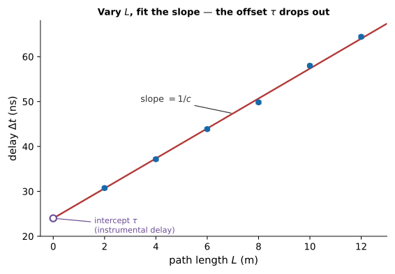
A plot of delay against path length: the data fall on a straight line whose slope is 1/c and whose y-intercept is the fixed instrumental delay tau, which is unknown but drops out of the slope. — Figure 2.1:The slope-fit trick. $\tau$ shifts every point up by the same fixed amount, so it changes the intercept but not the slope — the fit recovers $c$ without ever needing to know $\tau$ .

What limits you¶

An oscilloscope of analog bandwidth $B$ has a 10–90% rise time of about

t_r \approx \frac{0.35}{B},

(2.3)

so a $100\ \text{MHz}$ instrument smears every edge over roughly $3.5\ \text{ns}$ — about a meter of light travel. This does not mean you cannot do better than a meter. A smeared edge can still be located to a fraction of its rise time, because averaging many acquisitions beats down the noise on the edge and the scope interpolates between samples. In practice, with enough signal, sampling, and a stable trigger, locating an edge to a fraction of a nanosecond may be possible. Measure that timing scatter on your actual setup. Across a $10\ \text{m}$ path change, $0.4\ \text{ns}$ is about 1.2% of the $33\ \text{ns}$ flight-time change.

The other contributors are: the sampling interval (use the fastest time base that still shows both edges), trigger jitter (trigger on the reference channel, which is bright and fast), and — the one students usually forget — the unequal electrical lengths of the two BNC cables. Signal travels in typical RG-58 at about $0.66c$ , so a $30\ \text{cm}$ cable mismatch changes the channel offset by about $1.5\ \text{ns}$ . If the cables remain fixed throughout the path-length series, that offset changes the intercept, not the fitted speed. Measure the cables and swap them once as a control; a path-dependent change in electronics or detector response would affect the slope.

Pre-lab¶

Apparatus¶

Fast pulsed source: a laser diode module driven by a $\sim1\ \text{MHz}$ square wave with a fast edge, or a red/IR LED driven hard by a MOSFET gate-driver. Check source current and edge-speed requirements; a microcontroller GPIO may not drive the source adequately by itself.
Function generator or microcontroller producing the drive pulse
Two photodiodes with fast amplifiers (target bandwidth at least 200 MHz; a 12 MHz PDA36A2 would broaden the edge substantially and make the target timing precision harder to reach)
Oscilloscope, $\ge 100\ \text{MHz}$ , with averaging
Two front-surface mirrors on adjustable mounts, to fold the path
Tape measure ( $\pm 2\ \text{mm}$ ) and a target card
Two BNC cables of measured, ideally equal, length

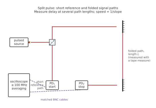
A pulsed source is split at a beamsplitter into a short reference path to one photodiode and a folded path via two mirrors to a second photodiode, both feeding a fast oscilloscope. — Figure 2.2:The time-of-flight bench. A fast pulse is split into a fixed reference path and a folded path of measured length $L$ ; the inverse slope of delay versus $L$ estimates the propagation speed while fixed channel delays enter the intercept.

Procedure¶

Before you route the beam¶

Trace the short reference path and folded signal path in Figure 2.2, then sketch the actual room layout with a label for every straight segment. Your measured $L$ will be the sum of those segments, not the source-to-detector displacement.
Place the beam below eye level, mark the occupied floor area, and install a block immediately behind the signal detector. Switch the source off while a mirror or detector is being moved.
Measure and label the two BNC cables before connecting them. Record detector model, amplifier gain, bandwidth limit, probe attenuation, and scope sample rate; a saved waveform without these settings is not reproducible.
Prepare a table with path length, uncertainty, delay, delay scatter, signal amplitude, averaging count, and file name. Reserve rows for at least eight lengths plus the cable-swap control.
Save one unaveraged waveform and one averaged waveform at the shortest path. These establish the raw noise level and show exactly what the averaging did.

Part A — Setting up the two channels¶

Mount the source. Split a small fraction of its output onto the reference photodiode a few centimeters away — a glass slide at $45°$ is enough. This channel defines $t_0$ and removes any drift in the source’s turn-on time.
Send the main beam across the room, fold it with the two mirrors, and bring it back onto the signal photodiode. Start with the shortest workable path, about $2\ \text{m}$ total.
Trigger the scope on the reference channel. Set both channels to the same vertical scale and DC coupling.
Turn on averaging (128 acquisitions is a starting point) and compare the timing scatter. Averaging reduces random noise; it does not restore edge speed lost to limited detector or oscilloscope bandwidth.

[ ] Checkpoint 1. Show the instructor two clean, averaged edges with a stable trigger. If the signal edge is noisy, the beam is possibly off-center; check beam centering, source stability, and electronic noise before changing the amplifier gain.

Part B — The delay measurement¶

Define your timing criterion before taking data and use it unchanged for every measurement. The 50%-amplitude crossing of the rising edge is a good choice; the peak is a bad one, because the two pulses have different shapes. Most scopes will do this automatically with a delay or “phase” measurement between channels.
Record $\Delta t$ and its scatter over several acquisitions.
Measure the total optical path $L$ from the source, via both mirrors, to the signal detector. Measure it with a tape, along the beam, and record the uncertainty. Do not forget the short leg from the beamsplitter to the reference detector — it enters $\tau$ , so it must not change between runs.
Move one mirror to lengthen the path by roughly $1\ \text{m}$ , realign onto the detector, and repeat. Collect at least eight path lengths spanning as large a range as the room allows.

Part C — Controls¶

Swap the two BNC cables and repeat one measurement. If cable delay is the only change, the measured delay shifts by twice the original cable offset. This checks the intercept contribution; a fixed offset cancels from the fitted slope. Restore the original cabling for the series.
Block the main beam and confirm that the pulse correlated with the reference disappears from the signal channel. A remaining correlated pulse suggests electrical crosstalk; find and remove it before fitting. Background and detector noise need not disappear completely.
If time allows, repeat one path length with the averaging turned off, to see what averaging bought you.

Analysis¶

Fit $\Delta t = L/c + \tau$ with both parameters free.

import numpy as np
from scipy.optimize import curve_fit

L   = np.array([...])          # total optical path, meters
sL  = np.array([...])          # uncertainty, meters
dt  = np.array([...])          # measured delay, seconds
sdt = np.array([...])          # uncertainty, seconds

model = lambda L, inv_c, tau: inv_c * L + tau
p0    = [1 / 3e8, 0.0]
popt, pcov = curve_fit(model, L, dt, p0=p0, sigma=sdt, absolute_sigma=True)

inv_c, tau = popt
s_inv_c    = np.sqrt(pcov[0, 0])
c, sc      = 1 / inv_c, s_inv_c / inv_c**2      # note the 1/x propagation
print(f"c   = {c:.4g} +/- {sc:.2g} m/s")
print(f"tau = {tau*1e9:.2f} ns")

resid = (dt - model(L, *popt)) / sdt
print(f"chi2/nu = {np.sum(resid**2) / (len(L) - 2):.2f}")

Note the propagation in the calculation of sc: the fit parameter is $1/c$ , so $\sigma_c = \sigma_{1/c}/(1/c)^2$ . Fitting $1/c$ rather than $c$ keeps the model linear; the covariance matrix still depends on a suitable uncertainty model and stable channel delays.

Because $L$ also carries uncertainty, check whether it matters: the effective uncertainty on $\Delta t$ from a position error is $\sigma_L/c$ . For $\sigma_L = 5\ \text{mm}$ this is $17\ \text{ps}$ , far below your timing uncertainty — so position error is negligible here, and you should say so rather than silently ignoring it.

Plot the residuals. A curved pattern suggests an effect that changes with path length, such as detector illumination, pulse shape, or a changing electronic delay. Investigate before interpreting the fitted speed.

Post-lab questions¶

Going further¶

Propagation speed in coaxial cable. Send the same pulse down a long spool of RG-58 and measure the delay per meter. You should get $v \approx 0.66c$ , and $v = c/\sqrt{\varepsilon_r}$ then gives you the dielectric constant of polyethylene. Same apparatus, one extra cable, ten minutes.
Speed of light in a medium. Put a $1\ \text{m}$ tube of water in the beam path and measure the extra delay. Expect $n = 1.33$ , so a $1.1\ \text{ns}$ shift — right at the edge of what you can resolve, which makes it a good exercise in whether you believe your own error bars.
Rømer’s method, from your desk. Public ephemerides give the eclipse times of Io over a year. Fitting the residual against Earth–Jupiter distance reproduces the 1676 measurement in an afternoon of Python and no apparatus at all.