Experiment 12 — Molecular Fluorescence, the Stokes Shift, and Franck–Condon¶
Objectives¶
By the end of this experiment you should be able to:
Measure an absorption spectrum and verify the Beer–Lambert law over a range of concentrations.
Measure a fluorescence emission spectrum and determine the Stokes shift.
Interpret the Stokes shift and test whether the lowest-energy absorption band and emission band are approximately mirror symmetric.
Estimate a vibrational energy quantum only if a resolved, assigned vibronic progression is present; otherwise explain the resolution limit.
Textbook connection¶
Read §12.4–12.7. Chapter 12 builds molecular energy levels as a hierarchy: electronic states separated by a few eV, vibrational levels within them separated by tenths of an eV, and rotational levels by meV. These energy scales and the fact that electronic transitions are fast relative to nuclear motion help explain the spectra measured here.
Theory¶
Why absorption and emission are not at the same wavelength¶
The Franck–Condon principle approximates an electronic transition as fast compared with nuclear motion. On a potential-energy diagram, the most probable transitions are therefore vertical.
The excited electronic state may have a different equilibrium nuclear geometry from the ground state. A vertical transition from a populated ground-state vibrational level can therefore populate several excited-state levels. Vibrational and solvent relaxation often precede fluorescence from the lowest excited singlet state. The vertical emission transition can then populate vibrationally excited ground-state levels, which relax afterward.
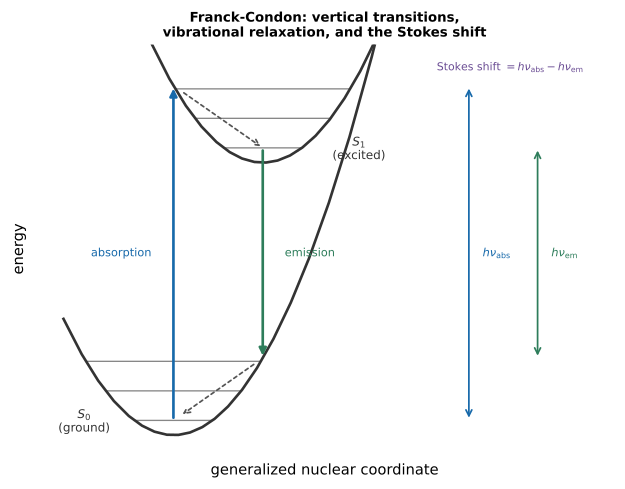
Figure 12.1:An idealized Franck–Condon cycle. Vertical arrows show electronic transitions; dashed arrows show relaxation between them. The pictured excitation and emission photons differ in energy. Real bands also depend on solvent reorganization, populated starting levels, and other decay channels.
For the usual relaxed fluorescence from these dilute dyes, the emission-band maximum is expected at lower photon energy than the corresponding absorption-band maximum. Their difference is the Stokes shift,
usually reported in or eV so it can be compared across spectral regions. Also report the two peak wavelengths. Individual photons can overlap or even appear on the anti-Stokes side; the difference of band maxima is an operational measurement, not a fixed energy lost by every photon.
The mirror-image rule¶
For comparable potential shapes and the same emitting species, the lowest-energy absorption band and corrected emission band may look roughly mirror symmetric on an energy or wavenumber axis. Strong solvent effects, overlapping electronic bands, reabsorption, or different chemical forms can spoil this approximation. Estimate a 0–0 origin from mirror symmetry only if those conditions and the spectral overlap support it; otherwise report the observed peak separation without an invented origin.
Beer–Lambert¶
Light of intensity entering a sample of path length and concentration emerges with
where is the absorbance and the molar absorptivity, in . Linear versus requires a stable absorbing species, known path length, and a detector operating above its dark and stray-light floor. Chemical changes, aggregation, scattering, and instrumental stray light can produce different deviations; the concentration series tests the range over which the relation holds.
Pre-lab¶
Apparatus¶
Calibrated spectrometer with detector, cuvette mount, and suitable visible response: a USB fiber spectrometer or a detector-equipped EDU-SPEB2 setup with suitable coupling. The EDU-SPEB2 viewing screen alone cannot record quantitative absorbance or emission spectra.
Broadband white LED or tungsten lamp, for the absorption measurement
Excitation LED matched to the dye: for example, a blue LED near 470 nm for fluorescein, or a UV LED near 365 nm for quinine if the optics and cuvette transmit there. A second excitation source is optional.
Long-pass filter chosen to reject the selected excitation wavelength while passing the emission band; record its transmission range
cuvettes with suitable UV transmission if needed; volumetric glassware; micropipettes
A dye with known concentration and fixed solvent/pH across dilutions: fluorescein in dilute base or quinine sulfate in dilute sulfuric acid. Tonic water can be used for a qualitative spectrum, but its unknown quinine concentration cannot yield a molar absorptivity. Rhodamine 6G in ethanol or chlorophyll extract in acetone are optional prepared samples.
Cuvette rack, lint-free wipes
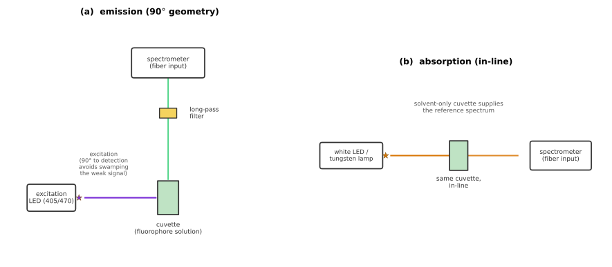
Figure 12.2:Two geometries, one cuvette. (a) Excitation at 90 degrees to detection, with a long-pass filter, keeps the weak fluorescence from being swamped by scattered excitation light. (b) In-line transmission gives the absorption spectrum.
Procedure¶
Before you prepare the dilution series¶
Use the two panels of Figure 12.2 as separate layouts: in-line lamp–cuvette–spectrometer for absorption, and 90-degree LED–cuvette–filter–spectrometer for emission. Do not use an absorption reference spectrum to correct the emission geometry.
Label every cuvette and dilution before pipetting. Keep solvent and pH constant, and prepare a dilution table with stock concentration, transfer volume, final volume, concentration, and propagated uncertainty.
Fix cuvette orientation with a small mark on a frosted face. Rinse with the next solution, fill to the same height, remove bubbles, and wipe the clear faces with lint-free tissue before every reading.
Warm up the light sources and spectrometer, then record integration time, gain, fiber position, filter, and file name. Clamp the fibers so geometry cannot drift across the concentration series.
Define a saturation threshold and a minimum useful signal before collecting the series. Retake dark and solvent reference data whenever integration time, gain, source, or transmission geometry changes; collect a matching solvent-only fluorescence blank whenever excitation, filter, or collection geometry changes.
Part A — Spectrometer setup¶
Record a dark spectrum (source blocked) and a reference spectrum (solvent-only cuvette in the beam). Every absorbance is computed from these two, so retake them whenever the geometry or integration time changes.
Verify wavelength calibration against a suitable known narrow line; an uncalibrated LED peak is not a wavelength standard.
Confirm that both reference and sample signals stay below detector saturation and above the measured dark/stray-light floor over the wavelengths used for fitting.
[ ] Checkpoint 1. Show the instructor your dark and reference spectra, and a solvent-only “absorbance” spectrum, which should be flat and near zero. A sloping baseline here will masquerade as a spectral feature later.
Part B — Absorption and Beer–Lambert¶
Prepare at least six known concentrations. Use the expected absorptivity and measured signal floor to aim for several peak absorbances from about 0.05 to 1.5; include a more concentrated sample only if useful for investigating departures. Record actual volumes and their uncertainties. Serial dilutions share stock and transfer uncertainties.
Record the absorbance spectrum of each. Note the peak wavelength and peak absorbance.
Plot peak absorbance against concentration and inspect residuals from the low-concentration line. Check whether departures follow the instrument’s dark or stray-light floor, scattering, a pH change, or a reproducible spectral-shape change. A moving peak alone does not prove aggregation.
Part C — Emission¶
Choose a dilute sample, ideally across the excitation path, and check absorbance across the emission band. At , about 79% of incident light traverses a 1 cm path; stronger absorption changes where fluorescence originates. Reabsorption of emitted light can also alter its profile: together these are inner-filter effects.
Illuminate from the side, at to the collection axis, so that unabsorbed excitation light does not enter the spectrometer.
Put the matched long-pass filter before the collection fiber and verify that it passes the emission peak rather than clipping the blue side.
Record a dark and a solvent-only fluorescence blank at the same settings and subtract both appropriately. Check residual excitation leakage, Raman features, and filter or solvent background.
If a second source also excites the same dye, repeat with its matched filter and blank. Compare normalized, background-corrected band shapes over their common passband. Kasha’s rule concerns relaxation to the lowest excited state; different apparent spectra can also arise from filters, detector response, or different chemical forms.
Part D — Concentration and quenching¶
Record emission spectra across the dilution series at fixed excitation power, filter, and geometry. Plot background-corrected integrated emission against concentration. Expect an approximately linear low- concentration region if detector response and quantum yield are stable; a plateau or downturn at higher concentration can reflect inner-filter effects, quenching, aggregation, or detector saturation. Use dilution and geometry checks to distinguish them.
Part E (optional) — Chlorophyll¶
If a prepared chlorophyll extract and approved solvent-handling setup are available, record its absorption and emission. Compare only an assigned absorption/emission pair, accounting for overlapping pigments, reabsorption, and solvent effects before interpreting the shift.
Analysis¶
Beer–Lambert¶
import numpy as np
from scipy.optimize import curve_fit

A  = np.array([...])           # peak absorbance
sA = np.array([...])
c  = np.array([...])           # molarity
sc = np.array([...])
ell_cm, sell_cm = 1.00, 0.01   # replace with measured path and uncertainty

sel = np.array([...], dtype=bool)  # select a range after checking floor and residuals
popt, pcov = curve_fit(lambda c, A0, m: A0 + m * c,
                       c[sel], A[sel], sigma=sA[sel], absolute_sigma=True)
A0, m = popt
eps = m / ell_cm
seps = np.hypot(np.sqrt(pcov[1, 1]) / ell_cm,
               abs(eps) * sell_cm / ell_cm)
Plot all points and fit a justified range whose transmission remains above the measured floor. Show the excluded points and residuals. A significant nonzero intercept calls for a blank or baseline check; do not silently force it to zero. The code propagates fit and path-length uncertainty but treats concentrations as exact. If their uncertainties matter, fit with a method that includes uncertainty in both axes or propagate the common stock and dilution errors by simulation. Report with its uncertainty and compare with a literature value for the same dye form, solvent, and pH.
Stokes shift and the mirror line¶
Convert both wavelength axes to wavenumber. Absorbance is dimensionless at each wavelength, so relabel its axis without multiplying the ordinates. For an emission spectrum calibrated as spectral density per nm, preserve area when changing axes: for in . Raw counts per detector pixel require a wavelength-bin calibration before using that Jacobian. Correct the detector’s wavelength response and remove background before comparing band shapes or quoting a precise peak shift.
nu_abs = 1e7 / lam_abs_nm                # cm^-1; A_abs stays unchanged
nu_em  = 1e7 / lam_em_nm
F_nu   = F_lam_per_nm * lam_em_nm**2 / 1e7
Locate each band maximum using a documented local fit or smoothing window that is wider than the noise but narrower than the band; compare reasonable window choices. Report with uncertainty from calibration, noise, and peak-finding choices.
If an isolated lowest-energy absorption band and corrected emission band have sufficient overlap, reflect one about a trial wavenumber and test whether a plausible mirror line aligns their resolved features. State the fit interval and sensitivity to background correction. If the bands do not support this test, report that limit. Half the Stokes shift equals the relaxation energy on either side only in the ideal equal-curvature displaced-harmonic model pictured above.
A vibrational quantum¶
If your spectra show a resolved, assigned vibronic progression, measure successive peak spacings. A nearly constant spacing may estimate the coupled mode’s vibrational quantum ; report it in and meV. Compare it with : the ground vibrational level dominates only when that mode’s spacing is large compared with .
If no structure is resolved, state the instrument resolution and observed band width. Overlapping modes and broadening can hide even widely separated quanta, so an unresolved band alone gives no bound on their spacing.
Post-lab questions¶
Going further¶
Fluorescence quantum yield. Comparing integrated emission against a standard of published yield under specified solvent, pH, temperature, and excitation conditions can give the fraction of absorbed photons re-emitted. Match low absorbances, correct integrated emission for detector response and background, and account for any refractive-index difference.
Iodine vapor. With a sealed I cell and enough spectral range and resolution, assigned vibronic bands can give vibrational spacings. A Morse fit and Birge–Sponer extrapolation require many reliable assignments and a justified dissociation limit; a few unresolved band heads are insufficient.
Fluorescence lifetime. A nanosecond decay requires a pulsed source, fast detector, sufficient recording bandwidth, and a measured instrument response. If these are available, fit the decay after accounting for that response. Together with an independently measured quantum yield, a single-exponential lifetime can estimate radiative and nonradiative rates.