Experiment 5 — Diffraction and the Resolution Limit¶
Objectives¶
By the end of this experiment you should be able to:
Fit a single-slit diffraction profile and extract the slit width with an uncertainty.
Use a diffraction grating to measure a wavelength, and explain why a grating outperforms a double slit for this purpose.
Measure a sub-micrometre periodic structure — the track pitch of an optical disc — with a laser and a ruler.
State the Rayleigh criterion, compare it with a visual threshold, and explain what also limits a telescope, a microscope, and your own eye.
Textbook connection¶
Read §5.1–5.6. The Rayleigh criterion introduced there is the reason Chapter 7’s electron microscope is worth building, and the grating equation is the instrument that Experiments 10, 11, and 12 all depend on. Treat this week as calibration for the second half of the course.
Theory¶
The single slit¶
A slit of width produces minima where
(note: is not a minimum — it is the central maximum), and an intensity profile
The central maximum is twice as wide as the others and contains about 90% of the transmitted power. Narrowing the slit widens the pattern — the inverse relationship between aperture and angular spread that, translated into momentum language in Chapter 7, becomes the uncertainty principle.
The circular aperture¶
For a circular aperture of diameter the pattern is the Airy disc, and the first zero falls at
The 1.22 is the first positive zero of divided by , for an ideal, uniformly illuminated circular aperture. It differs from the single-slit result, so use the right aperture model when inferring .
The Rayleigh criterion¶
Two incoherent point sources are said to be just resolved when the first zero of one Airy pattern falls on the central maximum of the other:
This is a convention for two equally bright, incoherent point sources in an ideal circular-aperture image. Contrast, noise, aberrations, detector sampling, and the source itself affect a real threshold. A known point-spread function can support more precise localization under suitable conditions, but the Rayleigh angle remains a useful diffraction scale. Electron microscopes gain from much shorter electron wavelengths, while their lenses impose other limits.
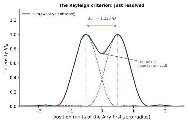
Figure 5.1:Just resolved under the Rayleigh convention. Each source alone (dashed) has an Airy profile; separated by , their summed intensity (solid) has a central dip about 26.5% below the peaks. The figure is a one-dimensional cross section of the circular pattern.
The grating¶
equally spaced slits of pitch give maxima at
the same condition as two slits — but the maxima are far narrower, with angular width . That sharpening, not the position of the maxima, is what makes a grating a spectroscopic instrument. Its resolving power is
so an ideal grating with a measured illuminated width has and a first-order grating limit of at . A narrow laser beam may illuminate fewer grooves, and a spectrometer’s entrance slit, optics, alignment, and detector can make its actual resolution worse. See the Feynman grating derivation and this spectrograph laboratory guide.
Optical discs as gratings¶
The data tracks of a CD or DVD form a reflection grating. Nominal pitches are for CD, for DVD, and for Blu-ray. For a DVD, , so first order appears at — a large angle where the small-angle approximation fails completely and you must measure the actual angle. For Blu-ray at , and no first order can propagate in air at normal incidence in the simple grating model. Failure to see an order alone is not proof of this inequality: weak efficiency, disc cover layers, alignment, and limited angular coverage can also hide one. The nominal pitches are tabulated in this Stony Brook optical-disc teaching project.
Pre-lab¶
Apparatus¶
Diode laser, (with the uncertainty you established in The Michelson Interferometer and the Ether Null Result)
Single slits of several widths; circular apertures; the “unknown” slide
Transmission grating, – (use a genuine transmission grating; a reflective grating requires a different geometry)
CD, DVD, and optionally a Blu-ray disc, mounted for a separately aligned reflection measurement; do not peel or cut discs
Rotation stage or a large protractor and a meter stick, for large angles
Camera or scanning photodiode; screen
Two small, measured pinholes on a card with a diffuse lamp behind, for the visual threshold comparison; a calibrated variable iris or aperture set
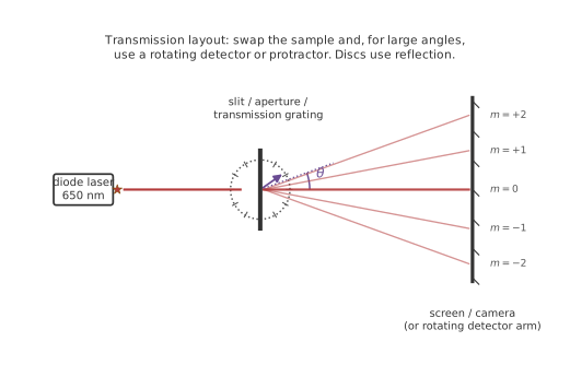
Figure 5.2:The transmission-diffraction bench for the slit, aperture, and grating. Measure large angles with a rotating detector or protractor. Optical discs require a separate reflection layout, with the diffracted orders detected on the incident side.
Procedure¶
Before you take diffraction data¶
Use Figure 5.2 to plan the transmission measurements. Record the slit, aperture, or grating installed for each file. Draw and separately align the disc reflection layout before collecting disc data.
Align the rail with no sample present and mark the zero-order beam position. Recheck that mark after every sample change; a shifted zero biases all measured angles and radii.
Copy the nominal slit widths, aperture diameters, and grating line density into a table, but keep them labeled “nominal” until compared with your measured values.
Record a dark frame and a spatial calibration at the screen plane. For profiles, lock the camera settings or record the photodiode gain and step size so intensities can be compared.
For every pattern, save the overview and the quantitative positions or profile used in your analysis. Note which orders or minima are visible before changing the apparatus; do not infer unseen orders from a diagram.
Part A — Single slit¶
Set and illuminate a slit of known width.
Record the positions of visible minima on both sides of the center, through if the field and dynamic range permit. The separation of the and minima spans eight orders; divide by eight in the small-angle limit, or fit the exact-angle relation below.
Take a quantitative profile with the camera or the scanning photodiode, as in Interference of Light. Watch for saturation.
Repeat with two more slit widths, and with the unknown.
[ ] Checkpoint 1. Confirm with the instructor that your widest and narrowest slits give patterns of the expected relative widths. If narrowing the slit does not widen the pattern, check alignment, source illumination, detector field, and whether you located the minima.
Part B — Circular aperture and the Airy disc¶
Replace the slit with a circular aperture. Photograph the Airy pattern with a long enough exposure to see the first dark ring and with a shorter exposure to keep the center unsaturated. Use each image for the feature it resolves; retain its exposure and scale rather than merging intensities without a calibrated response.
Measure the radius of the first dark ring, and extract from (5.3). Compare with a direct measurement of the aperture under a traveling microscope if one is available.
Part C — The grating¶
Mount the grating on the rotation stage with the beam at normal incidence. Check the grating normal using the reflected zero order or the mount’s reference, then compare the and angles as a symmetry check. A mismatch can indicate tilt or an angle-zero error.
Measure for every visible order, on both sides.
Using the specified line density, compute ; then use the independently measured from Experiment 1 to infer line density. Compare with uncertainties, including the specification’s tolerance if given.
Part D — Optical discs¶
Mount the CD in reflection near normal incidence. Block the specular return beam and locate first orders on the incident side using a rotating detector or screen. Measure signed angles from the reflected zero-order direction, or measure spot position and screen distance and compute . Check symmetry before using the normal-incidence formula.
Repeat for the DVD. Note that the angle is large: do not use the small-angle approximation, and measure the geometry carefully enough that you know to a degree or better.
If a Blu-ray disc is available, scan the accessible incident-side angles for a first order and record the angular coverage and detection limit. An absent spot is consistent with at normal incidence but alone does not establish a pitch bound.
Part E — Resolution¶
Set up two small pinholes with measured separation and diameter, back-illuminated by a diffuse lamp at measured distance. Avoid a coherent laser source, which would produce a different two-source pattern.
View them through a calibrated variable iris near the eye. Record the iris diameter at which they merge while keeping ambient light and viewing distance fixed. Note the actual eye pupil and pinhole sizes as practical limitations.
Repeat with both observers. Report trial-to-trial and observer variation, plus iris calibration and geometry uncertainty; a visual threshold is not a direct measurement of the ideal Rayleigh boundary.
Analysis¶
Slit width from minima¶
The minima positions satisfy in the small-angle limit, but do not use small angles if you do not have to. Fit
as a straight line in signed order ; its slope is . Allow a small intercept to diagnose a mislocated pattern center.
import numpy as np
from scipy.optimize import curve_fit

m  = np.array([-4, -3, -2, -1, 1, 2, 3, 4])
y  = np.array([...])            # minima positions relative to center, meters
sy = np.array([...])
sin_th  = y / np.sqrt(y**2 + L**2)
ssin_th = sy * L**2 / (y**2 + L**2)**1.5      # independent position errors

popt, pcov = curve_fit(lambda m, b, s: b + s*m, m, sin_th,
                       sigma=ssin_th, absolute_sigma=True)
slope = popt[1]
a  = lam / slope
sa = a * np.sqrt((np.sqrt(pcov[1,1])/slope)**2 + (slam/lam)**2)
Here y, sy, L, lam, and slam are your measured positions, their
standard uncertainties, screen distance, wavelength, and wavelength
uncertainty in SI units. Refit at plausible and center-position limits
to include their shared systematic effects; do not put one common
error into every independent sigma entry. Inspect the intercept and
residuals. Use absolute_sigma=True only for defensible absolute standard
uncertainties. Then fit the full profile with (5.2) if the
detector response is linear enough, and compare the two values of with
their shared wavelength and distance errors. Saturation or camera processing
can distort an intensity fit.
Grating and discs¶
For a near-normal transmission grating, fit signed against signed with an intercept; its slope is . A nonzero intercept or differing estimates may indicate angle-zero or incidence error. Common wavelength and angle calibrations correlate the inferred pitches, so do not treat all orders as independent measurements when quoting uncertainty. For discs, use the reflected zero-order direction and the separately drawn reflection geometry. The same simple form applies only after normal incidence and an appropriate diffraction order have been established.
Resolution¶
Compare your measured threshold iris diameter with the prediction from (5.4), using the measured pinhole separation and distance. Report the ratio measured/predicted with the uncertainties you can support. Discuss pinhole size, eye optics, pupil diameter, brightness, and observer judgment before interpreting disagreement with the ideal criterion.
Post-lab questions¶
Going further¶
Babinet’s principle. Replace the slit with a wire of the same width. The diffraction patterns are identical away from the center — a result that surprises everyone the first time and follows in one line from linearity of the wave equation. Measuring a wire diameter this way is a genuinely useful technique.
Measure a hair, a spider silk, or a fiber. Same principle, and it connects directly to the air-wedge measurement of Week 4. Two independent measurements of the same hair make a nice paragraph in a report.
Poisson’s bright spot. Put an opaque circular obstacle in an expanded clean beam and look at the center of its shadow. The bright spot there was advanced in 1818 as a reductio ad absurdum against Fresnel’s wave theory, and then observed. It requires a clean beam and a good circular edge, and it is worth the trouble.