The Quantum Eraser and Complementarity - Modern Physics Laboratory

Experiment 7 — The Quantum Eraser and Complementarity¶

Objectives¶

By the end of this experiment you should be able to:

Show how orthogonal slit polarizers remove interference from the full beam and how a downstream analyzer selects subsets with fringes.
Measure fringe visibility quantitatively from an intensity profile.
Measure both fringe visibility and transmitted-path bias independently, and compare their trade-off with $V^2+D^2\le1$ for this optical layout.
State precisely what this experiment does and does not establish about the quantum nature of light — a distinction that a great many popular accounts get wrong.

Textbook connection¶

Read §7.1–7.5. Chapter 7 argues that particles have wave properties; this experiment uses polarized light to make two paths distinguishable and then selects a common polarization to recover interference in transmitted subsets. This is a classical-wave analog of a quantum eraser, with de Broglie wavelengths treated separately in the computational analysis.

Theory¶

Which-path information destroys interference¶

Prepare incident polarization at $45°$ to the horizontal and vertical axes so both slits can receive comparable power. Put orthogonal linear polarizers over the two slits — horizontal over slit 1, vertical over slit 2. The two emerging fields are now orthogonally polarized, and orthogonal polarizations do not interfere: the cross term in $|E_1 + E_2|^2$ contains $\hat{e}_1 \cdot \hat{e}_2 = 0$ . The fringes vanish, leaving the sum of the two single-slit patterns.

The polarization carries a path marker. Without a downstream analyzer, the full intensity has no cross term even if no observer checks polarization. This statement concerns the full, unselected beam; a selected polarization subset can have interference.

Erasing the mark¶

Now place a third polarizer, at $45°$ , after the slits. It projects both beams onto a common polarization. In the transmitted subset, the original polarization marker no longer distinguishes the slits; if their incident powers are balanced, either path contributes equally. The fringes return among the transmitted light, while the analyzer discards other light.

Rotate the analyzer to $-45°$ and the fringes return again, but shifted by half a period — bright where they were dark. This is the crucial control. Adding the two orthogonal-analyzer profiles reproduces the marked, no-analyzer profile in the ideal stable setup. They are complementary polarization projections; neither creates light or changes the earlier path.

Visibility and distinguishability¶

Define the fringe visibility from the intensity profile:

V = \frac{I_{\max} - I_{\min}}{I_{\max} + I_{\min}} .

(7.1)

For each analyzer angle $\theta$ , block one slit at a time and measure the dark-subtracted transmitted powers $P_1$ and $P_2$ in the same detector region. The path bias, or predictability, among the transmitted light is

D = \frac{|P_1-P_2|}{P_1+P_2} .

(7.2)

Here $D=0$ means no path preference and $D=1$ means only one slit contributes. Once both beams have passed the same ideal analyzer, the surviving polarization cannot reveal more path information, so this measured bias is the relevant distinguishability for this selected subset. For equal incident slit powers and ideal polarizers, $P_1\propto\cos^2\theta$ and $P_2\propto\sin^2\theta$ , giving

D = \left|\cos^2\theta - \sin^2\theta\right| = |\cos 2\theta| , \qquad V_{\rm ideal} = \left|\sin 2\theta\right| ,

(7.3)

so that

V_{\rm ideal}^{2} + D^{2} = 1 .

(7.4)

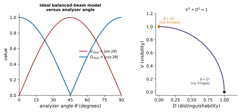
Ideal visibility V and transmitted-path bias D as functions of analyzer angle, and the unit-circle relation between them for balanced beams and ideal optics. — Figure 7.1:The curves show the **ideal balanced-beam model**. Measured visibility and the independently determined path bias can lie inside the unit-circle bound because of imperfect overlap, background, and polarization leakage.

For two beams with powers $P_1,P_2$ and otherwise perfect coherence, the largest possible visibility is $2\sqrt{P_1P_2}/(P_1+P_2)$ , so $V^2+D^2\le1$ when loss of coherence or overlap lowers the observed $V$ . This optical relation illustrates the quantitative duality developed by Englert, while this bright-beam experiment remains explainable by classical waves.

Pre-lab¶

Apparatus¶

Thorlabs EDU-QE1 kit for the $532\ \text{nm}$ laser and optical mounts. Its supplied Mach–Zehnder layout is different from this double-slit procedure. The instructor must provide and verify a separate double-slit mask with individually aligned H/V polarizer strips, a $45°$ input preparation polarizer or equivalent wave plate, and a rotatable analyzer.
Camera imaging a calibrated diffusing screen from outside the beam path, or a scanning photodiode with a narrow entrance slit. A bare sensor is suitable only if it captures enough fringe periods or can be scanned.
Rotation mount with a scale readable to $1°$ or better
Neutral-density filters, safe single-slit blockers, beam blocks, screen

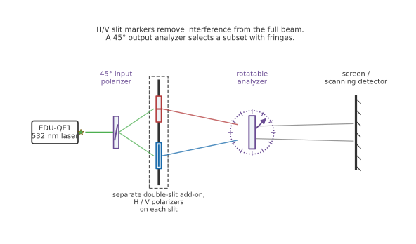
The EDU-QE1 laser passes through a 45-degree input polarizer before illuminating a separately mounted double slit with horizontal and vertical path polarizers; transmitted light passes through a rotatable analyzer to a screen or scanning detector. — Figure 7.2:The double-slit analog uses the EDU-QE1 source and mounts plus a separately verified slit-and-polarizer add-on. A $45°$ input polarization balances the marked paths. The output analyzer selects subsets; at $45°$ to H/V, both paths contribute to the transmitted fringes.

Procedure¶

Before you add the polarizers¶

Follow the component order in Figure 7.2: laser, input polarization preparation, double slit with its two path markers, output analyzer, then screen or detector. Record each transmission axis and verify the input gives comparable power through each marked slit with the other temporarily blocked. The figure’s axes are schematic, not calibration marks.
Center the expanded beam on both slits and mark the detector position. Once the baseline is satisfactory, tape or clamp every component except the analyzer rotation mount.
For screen imaging, calibrate position with a ruler in the screen plane. Lock camera exposure, gain, focus, and region of interest. Take a dark frame and retain the same response settings through Parts A–D.
Create a file-naming scheme containing analyzer angle, slit-block state, and trial number. Prepare a table for angle, full-pattern visibility, the two one-slit powers, $D$ , exposure, and file name.
Define $0°$ using extinction through one slit before collecting profiles. Approach each requested angle from the same rotation direction to limit mount backlash.

Part A — The baseline pattern¶

Use the kit laser and mounts with the instructor-approved separate double-slit add-on and screen or detector. Prepare the incident polarization at $45°$ to the future H/V markers. Do not install the two slit polarizers yet.
Record a clean interference pattern. Check for saturation and add an ND filter if needed — the visibility measurement is destroyed by clipping, because a clipped maximum makes $V$ artificially small.
Measure the fringe spacing and confirm it matches your pre-lab prediction. Record the baseline visibility.

[ ] Checkpoint 1. Show the instructor an unsaturated profile with enough visible periods for a stable visibility fit. A low baseline visibility can arise from uneven illumination, poor coherence, misalignment, camera response, or background; diagnose it before continuing.

Part B — Marking the path¶

Install the orthogonal polarizers over the two slits. The fringes should collapse into a smooth two-slit envelope with no oscillation.
Record the marked, no-analyzer profile. Measure any residual modulation; finite extinction, stray light, detector effects, and alignment can all contribute, so this is not a unique polarizer-quality measurement.
With beam power off while changing blockers, expose one slit at a time. Rotate the output analyzer on its mount to verify that the two paths transmit at orthogonal settings. Restore both slits before Part C.

Part C — Erasing¶

Install the analyzer after the slits and set it to $+45°$ . Record the profile: fringes should return.
Set it to $-45°$ and record again. The fringes should be shifted by half a period.
The essential control: after dark subtraction, add the two profiles from steps 7 and 8 point by point and compare with the marked, no-analyzer profile from step 5. Orthogonal ideal analyzer projections should sum to that profile if beam power, exposure, and geometry are stable. Check the total intensity as well as fringe cancellation.

[ ] Checkpoint 2. Show the instructor the two erased profiles and their sum.

Part D — The complementarity curve¶

Rotate the analyzer through at least twelve angles from $0°$ to $90°$ and record a two-slit profile at each. Keep exposure fixed when possible; if a different exposure is essential, normalize by measured time and verify response linearity. Record the angle to the mount’s precision.
At each angle, briefly block slit 2 and slit 1 in turn, recording dark-subtracted transmitted power from each path in the same detector region. Keep detector settings fixed, or correct for exposure time and verify linear response. Measure $D$ with (7.2) and $V$ from the full profile. Use (7.3) as a model prediction, not as the source of your measured $D$ . Plot measured $V$ against measured $D$ .

Part E (optional) — Interaction-free measurement¶

If the EDU-BT1 bomb-tester analogy kit is available, follow its manual to balance a Mach–Zehnder interferometer so one output is dark, then block one arm and record both output intensities. This bright-beam demonstration shows how blocking a path changes interference; it does not measure a single-photon interaction-free detection probability.

Analysis¶

Extracting visibility¶

Do not read $I_{\max}$ and $I_{\min}$ off a noisy plot by eye. Work with a linear, unsaturated detector response and one calibrated position axis. Estimate a smooth, positive envelope from the marked no-analyzer profile after dark subtraction, normalize its peak to 1, and use the same positions at every analyzer angle. Fit the known fringe frequency with cosine and sine terms:

import numpy as np

k = 2 * np.pi / fringe_spacing   # fixed from baseline; same units as y
X = np.column_stack([env, env*np.cos(k*y), env*np.sin(k*y),
                     np.ones_like(y)])
Xw = X / sprof[:, None]
coef = np.linalg.lstsq(Xw, prof / sprof, rcond=None)[0]
cov = np.linalg.inv(Xw.T @ Xw)   # absolute uncertainties in sprof
C, A, B, bg = coef
V = np.hypot(A, B) / C

# Propagate fitted-coefficient covariance, including the near-zero case.
rng = np.random.default_rng(7)
draws = rng.multivariate_normal(coef, cov, size=10000)
draws = draws[draws[:, 0] > 0]
v_draws = np.hypot(draws[:, 1], draws[:, 2]) / draws[:, 0]
v_lo, v_hi = np.quantile(v_draws, [0.16, 0.84])
v_upper = np.quantile(v_draws, 0.95)

Here env, y, prof, and sprof are measured arrays on one common position grid; env must not include its background. The fit separates smooth intensity, modulation, and a residual constant background. Fixing $k$ from Part A avoids chasing noise. The coefficient draws estimate profile noise conditional on the envelope and calibration. Near $V=0$ , the nonnegative amplitude estimator is biased upward, so report an upper bound such as v_upper when modulation is consistent with zero. Repeat with plausible envelopes and regions of interest to assess model sensitivity. A nonlinear sinc-squared model from Experiment 4 is another option if the slit width and detector response are well characterized.

The complementarity test¶

For each analyzer angle, calculate $D$ from the two measured one-slit powers with (7.2). Propagate their uncertainties, including dark background and power drift. Plot measured $V$ against measured $D$ , with error bars on both axes, and overlay the ideal unit-circle boundary. Calculate $V^2+D^2$ with uncertainty for each point. Compare measured $D$ and $V$ with the angle-only ideal predictions in (7.3); do not use those predictions as measurements.

The bound applies to the underlying optical state when $V$ and $D$ describe the same transmitted subset and the two single-slit profiles have compatible shapes across the fitted region. Noise and fit bias can put an estimate outside the circle. Investigate such a point’s uncertainty, background, normalization, detector response, and region choice before interpreting it. Limited coherence, spatial overlap, and polarization quality can put the underlying result inside the circle. Report the raw visibility: dividing it by the Part A baseline changes the measured quantity and is not a correction that preserves this bound.

The de Broglie calculation¶

Complete the pre-lab calculation properly, using the relativistic relation where it matters:

\lambda = \frac{h}{p}, \qquad pc = \sqrt{T^2 + 2Tm c^2} .

(7.5)

For a $50\ \text{eV}$ electron the relativistic correction is negligible; for a $100\ \text{keV}$ electron in a microscope it is not. Report both the non-relativistic and relativistic wavelengths at $100\ \text{keV}$ and quote the fractional difference.

Post-lab questions¶

Going further¶

Delayed-choice proposal. Design a test in which an active analyzer setting is switched after light passes the slits, with independently verified transit and switch timing. Predict the separately selected and summed detection profiles. Moving a static analyzer downstream alone does not establish delayed choice.
Quantum key distribution. The EDU-QCRY1 kit implements a BB84 analog with polarization states. Compare its basis-choice and error-rate concepts with the polarization projections here; the bright-beam bench does not implement a secure key exchange.
Photon counting. A heavily attenuated laser and a photon-counting detector can build a pattern from individual detection events, but the source still has laser photon statistics. For a claim about nonclassical single photons, add a characterized heralded or emitter-based source and an appropriate source-statistics measurement.