Planck's Constant from Light-Emitting Diodes

Experiment 6 — Planck’s Constant from Light-Emitting Diodes¶

Objectives¶

By the end of this experiment you should be able to:

Define a reproducible LED voltage proxy by extrapolating a selected part of its $I$ – $V$ curve, and quantify the fit-window dependence.
Measure an LED’s emission spectrum and use its peak rather than its nominal color.
Estimate Planck’s constant from voltage proxy against inverse wavelength, and assess how LED chemistry and wavelength calibration limit that estimate.
Determine an effective electrical-power exponent for a tungsten lamp and explain the conditions needed to interpret it as radiative $T^4$ behavior.

Textbook connection¶

Read §6.1–6.3. Chapter 6 introduces $h$ through blackbody radiation and the photoelectric effect. This LED measurement links photon energy to an approximate semiconductor voltage scale. The lamp part tests a consequence of thermal radiation, though an electrical-power curve alone is not a direct measurement of the emitted spectrum or a standalone proof of photon quanta.

An LED provides a useful contrast with the photoelectric effect. A photon can eject an electron from a surface when its energy exceeds a work function; an LED can emit a photon when injected carriers recombine across an energy gap. The LED voltage is affected by the junction and contacts, so its relation to photon energy is less direct than a photoelectric stopping-voltage relation.

Theory¶

The LED as a quantum energy converter¶

An injected electron and hole can recombine radiatively in a forward-biased LED. The photon energy is set mainly by the semiconductor transition energy; the following is an order-of-magnitude model, not an identity between terminal voltage and band gap:

eV_{\rm ideal} \sim E_g \sim hf = \frac{hc}{\lambda_p} .

(6.1)

There is no sharp electrical or optical turn-on. Define $V_{\text{proxy}}$ consistently from each measured curve. If the differences between this proxy and photon energy per charge are approximately common across the chosen LEDs, plotting it against $1/\lambda_p$ can approximate a line with slope $hc/e$ :

V_{\text{proxy}} \approx \frac{hc}{e}\cdot\frac{1}{\lambda_p} + V_{\text{offset}} .

(6.2)

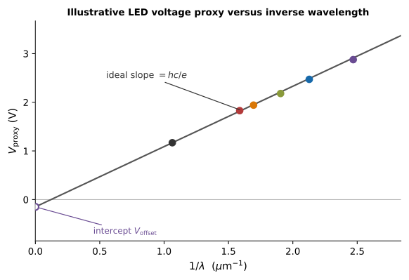
An illustrative scatter of LED voltage proxies against inverse peak wavelength lies near a line with the ideal slope hc/e; a sample intercept is marked but is not universal. — Figure 6.1:An illustrative six-LED plot. The line shows the ideal slope $hc/e$ under a common-offset assumption; real LED chemistries and proxy choices can change the slope and the sign of the intercept.

Why this is honest but imperfect¶

(6.1) is an approximation, and a report that does not say so is incomplete. Three effects matter:

No sharp threshold. A simple diode model is $I=I_s\left(e^{eV/nk_BT}-1\right)$ , where the ideality factor $n$ need not be the same for every LED or current range. There is no unique voltage at which current or light first appears. At room temperature $k_BT/e\approx26\ \text{mV}$ ; the voltage shift for a given current ratio is $n(k_BT/e)\ln(I_2/I_1)$ .

Series resistance. At high current the measured voltage includes $IR_s$ across the semiconductor and contacts. A high-current region may look linear, but its zero-current intercept is a procedure-dependent proxy, not an independent measurement of $E_g/e$ . Choose the fit window from observed linearity and test how much its intercept changes when the window moves.

Different spectra and junctions. The peak photon energy need not equal a single band-gap value, and its offset has no universal sign. Carrier distributions, alloy composition, quantum wells, reabsorption, and detector response can affect the peak and width. Red/amber and blue/green LEDs may use different semiconductor families, so treating all their offsets as one constant is the main model assumption to test.

An undergraduate LED demonstration can return a value of $h$ within tens of percent, but no accuracy target follows from this model alone. Report slope, intercept, residuals, and how the estimate changes with fit window and LED subset. An intercept close to zero or of either sign is possible. See the UCSB LED demonstration for an example of the method’s sensitivity to voltage definitions.

The Stefan–Boltzmann law¶

A tungsten filament at temperature $T$ radiates approximately

P_{\rm rad} = \varepsilon\sigma A\left(T^4 - T_{\text{amb}}^4\right) \approx \varepsilon\sigma A\,T^4

(6.3)

for $T\gg T_{\text{amb}}$ . Here $\varepsilon$ is an effective total emissivity, which can itself change with temperature. At steady state, electrical power $VI$ balances radiation plus conduction and any gas convection, so a fit to $VI$ measures an effective exponent. It estimates the radiative exponent only where those other losses are small and emissivity changes little over the chosen interval.

Estimate temperature from the filament’s resistance. Over roughly 300– $3000\ \text{K}$ , a useful empirical approximation for tungsten is

\frac{R(T)}{R_0} \approx \left(\frac{T}{T_0}\right)^{1.20}, \qquad T_0 = \text{measured room temperature},

(6.4)

with several-percent model error compared with tabulated tungsten resistivity. Use a table or compare with one if higher accuracy matters; allow for any non-tungsten lead resistance in the measured cold value. See the William & Mary tungsten-resistance table. If the hot-filament assumptions hold over a chosen interval, then

P_{\rm elec} = kT^{n} \quad\Longrightarrow\quad \ln P_{\rm elec} = n\ln T + \ln k ,

(6.5)

and a straight-line fit gives an effective $n$ . Compare it with 4 without assuming it must equal 4.

Pre-lab¶

Apparatus¶

At least five single-emitter LEDs with separated peaks, chosen within the calibrated spectrometer range: e.g. $\sim940$ , 630, 590, 525, 470, $405\ \text{nm}$ if those ends of the range can be measured reliably. Exclude phosphor-converted white LEDs from the single-transition fit: their broad spectrum combines a pump LED with phosphor emission.
Variable current-limited DC supply 0– $5\ \text{V}$ ; an automated sweep needs a suitable buffered output and measured, settled voltage/current
Two digital multimeters, or a microcontroller with two ADC channels and a known current-sense resistor
$100\ \Omega$ series resistor
EDU-SPEB2 spectrometer with a scanning detector (for example the EDU-SPEBCT1 extension and a suitable photodiode power meter), or a USB spectrometer with wavelength calibration and documented spectral response; a viewing screen alone cannot record the required spectra. Confirm range and sensitivity at every LED wavelength; the Thorlabs kit description lists a 400–1100 nm photodiode option.
Small tungsten filament lamp with a clear envelope, rated supply values, and a heat-resistant mat or tile
Bench supply capable of 0– $8\ \text{V}$ at $2\ \text{A}$ , with a four-wire or separate voltage-sense connection at the lamp terminals

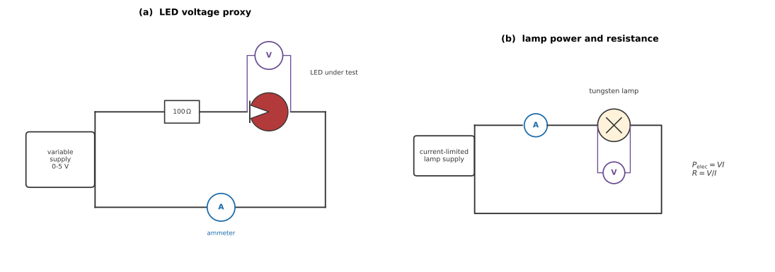
Panel (a), a current-limited LED circuit with current measured in series and voltage across the LED. Panel (b), a tungsten lamp circuit with current measured in series and voltage sensed at the lamp terminals for electrical-power and resistance thermometry. — Figure 6.2:Two electrical measurements. (a) The LED voltage proxy is extracted from current–voltage data and paired with a **separate LED emission spectrum**. (b) Lamp terminal voltage and current give resistance and electrical power; they do not directly measure emitted radiative power.

Procedure¶

Before you power a device¶

Identify the separate LED and lamp circuits in Figure 6.2. The LED spectrometer measures light from panel (a) separately; panel (b) measures lamp voltage and current, not its optical spectrum.
Sort the LEDs by package label and assign each a permanent ID. Never rely on emitted color alone, and do not mix devices after their spectra are taken.
With the supply off, verify resistor value and LED polarity with a meter. Set a current limit no higher than the lowest device’s rating, and no higher than $15\ \text{mA}$ for this procedure. Keep the series resistor even with a current-limited supply.
Prepare linked tables for LED ID, spectrum file, peak wavelength, FWHM, and every $(V,I)$ sweep. Record meter ranges and the resistor’s measured value with uncertainty.
Warm up the spectrometer as directed by its manufacturer. Keep the lamp unpowered until after its cold resistance is measured. Save dark spectra at every integration time and label all files as you take them; do not try to reconstruct LED identities afterward.
Plan scan time before starting. If a manually scanned spectrometer cannot cover every LED within the period, assign device subsets to teams using a common wavelength and response calibration, then share the measured files.

Part A — Emission spectra¶

Drive each LED at a safe, recorded current near $5\ \text{mA}$ if its rating permits and record its emission spectrum. Take a dark spectrum at the same integration setting; calibrate wavelength and account for the detector’s wavelength-dependent response before locating a peak.
For each usable spectrum, find the peak wavelength $\lambda_p$ and FWHM. Record both with calibration and resolution limits. The FWHM is not by itself a direct thermometer for the carriers.
Compare $\lambda_p$ with the device’s nominal value; do not assume a fixed difference. Use the measured, response-corrected peak for the fit, and exclude a device if its peak lies outside a reliable spectral range.

[ ] Checkpoint 1. Show the instructor your spectra with the peaks marked. A spectrum with a flat top is saturated; reduce the integration time and retake it.

Part B — LED voltage proxies¶

Wire the LED in series with the $100\ \Omega$ resistor across the supply. Measure the voltage across the LED alone (not across the pair) and the current through the resistor.
Sweep the supply upward and record at least 25 settled $(V,I)$ pairs, concentrated where the current rises steeply and through an approximately linear region if one exists. Stay below the device’s approved current limit and $15\ \text{mA}$ , whichever is smaller.
Use a comparable safe current window across LEDs where possible. If their ratings or curves prevent it, document the different windows and treat the resulting voltage-proxy comparison as less reliable.
Repeat for all LEDs.

Part C — The tungsten lamp¶

Measure the cold resistance $R_0$ of the lamp with a four-wire ohmmeter, or from a low-current $(V,I)$ measurement that does not heat the filament. Record the ambient temperature $T_0$ and assess any series resistance from leads or the lamp base.
Increase the lamp voltage in steps up to its rated value while limiting current during startup. Record lamp-terminal $V$ and $I$ after successive readings stabilize; do not assume a fixed ten-second settling time.
Take at least fifteen points, and take them over as wide a range as the lamp tolerates, since you are fitting an exponent.

Analysis¶

A voltage proxy by extrapolation¶

For each LED, fit a straight line to a reproducibly selected, approximately linear part of its measured $I$ – $V$ curve and extrapolate to $I=0$ . This defines $V_{\text{proxy}}$ , not a unique physical turn-on voltage. Check the residuals and use only a current range safe for every device in a common-window comparison. The example assumes sI contains independent, absolute standard uncertainties. If voltage errors are comparable to the fit’s horizontal scale, use an errors-in-both-variables model or refit at the voltage-calibration limits.

import numpy as np
from scipy.optimize import curve_fit

# Choose a common safe window after inspecting each curve; values are examples.
sel = (I > 5e-3) & (I < 12e-3)
assert sel.sum() >= 3
line = lambda V, m, b: m * V + b
popt, pcov = curve_fit(line, V[sel], I[sel], sigma=sI[sel], absolute_sigma=True)
m, b   = popt
V_proxy = -b / m
# full covariance propagation: V_proxy depends on both parameters
J      = np.array([b / m**2, -1 / m])
sV_proxy = np.sqrt(J @ pcov @ J)

State the window and each device’s rated current. Refit over at least one other safe, approximately linear window and record the changes in the voltage proxies and final slope. Do not use 8– $20\ \text{mA}$ when this procedure caps current at $15\ \text{mA}$ . If no suitable common interval exists, report that limit rather than forcing a fit.

Planck’s constant¶

inv_lam  = 1e-6 / lam_peak                    # 1/um; lam_peak is in meters
popt, pcov = curve_fit(lambda x, s, c: s * x + c, inv_lam, V_proxy,
                       sigma=sV_proxy, absolute_sigma=True)
slope, offset = popt
e = 1.602176634e-19
c_light = 299792458.0
h  = slope * e / (c_light * 1e6)
sh = np.sqrt(pcov[0, 0]) * e / (c_light * 1e6)

Here lam_peak, V_proxy, and sV_proxy are arrays, one value per usable LED. Report the slope, intercept, residuals, and conditional estimate of $h$ . The covariance above accounts only for voltage-proxy errors if those absolute standard uncertainties are justified. Refit after shifting calibrated wavelengths within their uncertainties; the $x$ values are not exact. Repeat with plausible fit windows and LED subsets, especially excluding one semiconductor family at a time. These model-sensitivity checks can dominate the formal sh. Avoid a standardized discrepancy unless a defensible combined uncertainty is known.

Lamp power and effective exponent¶

R = V_lamp / I_lamp
T = T0 * (R / R0) ** (1 / 1.20)
P_elec = V_lamp * I_lamp
fit = np.polyfit(np.log(T), np.log(P_elec), 1)  # exploratory slope only

Use lamp arrays here, separate from the LED sweep. The polyfit line is an exploratory slope only. $P_{\rm elec}$ and $T$ both depend on the same $V$ and $I$ , so their errors are correlated; a weighted fit treating them as independent is not a complete uncertainty analysis. Fit an identified hot-temperature interval. Repeat the full calculation at plausible meter, $R_0$ , and tungsten-calibration limits, and examine how the slope changes with fit interval. If you use a statistical fit with error bars, state its covariance assumptions; report residuals and $\chi^2_\nu$ only if those assumptions support them.

Exclude the lowest-temperature points and see whether $n$ moves. At lower $T$ , the ambient term, conduction, and possible gas convection become more important; changing tungsten emissivity affects even hot points. The direction of a slope change is not guaranteed. Report the measured trend and which effects these data can actually distinguish.

Post-lab questions¶

Going further¶

Temperature dependence of the voltage proxy. Cool an LED with the instructor’s approved, dry setup and repeat at a controlled current. The junction and band gap both change with temperature; determine the sign and size of $dV/dT$ for this device rather than assuming a universal coefficient.
Numerically integrate Planck’s law. Compute the ideal blackbody visible fraction as a function of $T$ , find its maximum, and compare with tungsten’s melting point. Real lamp efficiency also depends on emissivity, envelope, electrical losses, and how the eye weights different wavelengths.
The infrared LED. A $940\ \text{nm}$ LED extends your $1/\lambda$ range by a useful amount, and because it lies furthest from the visible LEDs it carries a great deal of leverage on the fitted slope. Measuring its spectrum requires a spectrometer that reaches into the near infrared — check the kit’s range before you trust the peak.