Interference of Light - Modern Physics Laboratory

Experiment 4 — Interference of Light¶

Objectives¶

By the end of this experiment you should be able to:

Predict and verify the fringe spacing of a two-slit interference pattern.
Fit a full two-slit intensity model, including the single-slit envelope, to a measured profile, and separate the roles of slit separation and slit width.
Estimate a sub-100-micrometre spacer thickness from air-wedge fringes and compare it with a micrometer measurement, when the wedge can be imaged.
Explain why interference requires coherence, and investigate how source width affects fringe visibility.

Textbook connection¶

Read §4.2–4.6. Chapter 4 develops the wave picture of light in the form that Chapters 6 and 7 will then have to be reconciled with. Everything you see this afternoon is wave behavior. With suitable single-photon source and detection equipment, arrivals build up the same spatial distribution one event at a time.

Theory¶

Two slits¶

Two narrow slits separated by $d$ , illuminated coherently, produce maxima where the path difference is a whole number of wavelengths:

d\sin\theta = m\lambda, \qquad m = 0, \pm1, \pm2,\ldots

(4.1)

On a screen at distance $L \gg d$ , with the small-angle approximation $\sin\theta \approx \tan\theta = y/L$ , the maxima fall at $y_m = m\lambda L/d$ and are evenly spaced by

\Delta y = \frac{\lambda L}{d}.

(4.2)

This is the working equation. Notice that it inverts nicely: measuring $\Delta y$ , $L$ , and $\lambda$ gives $d$ — you are using light to measure a distance far too small to read off with a ruler, which is the same trick as Experiment 1 in different clothing.

Two slits of finite width¶

Real slits have a width $a$ , and each one diffracts. The intensity is the two-slit interference pattern modulated by the single-slit envelope:

I(\theta) = I_0 \underbrace{\left[\frac{\sin(\pi a \sin\theta/\lambda)}{\pi a \sin\theta/\lambda}\right]^{2}}_{\text{single-slit envelope}} \underbrace{\cos^{2}\!\left(\frac{\pi d \sin\theta}{\lambda}\right)}_{\text{two-slit interference}} .

(4.3)

The envelope has its first zero at $\sin\theta = \lambda/a$ , and interference maxima that fall there are missing orders. On the interference-order axis $u=d\sin\theta/\lambda$ , the central envelope runs from $u=-d/a$ to $u=+d/a$ . The approximate interference orders inside it are the integers $m$ satisfying $|m|<d/a$ . If $d/a$ is an integer $k$ , the orders $m=\pm k$ are missing and there are $2k-1$ central orders; thus

\frac{d}{a} = \frac{\text{number of central interference orders}+1}{2} \qquad\text{when }d/a\text{ is an integer.}

(4.4)

A pattern with nine central orders is consistent with integer $d/a=5$ . For a noninteger ratio, counting orders only brackets $d/a$ ; locate the envelope zeros or fit the full profile to estimate it more precisely. The envelope shifts the exact bright-peak positions slightly away from integer $u$ , especially near its edges.

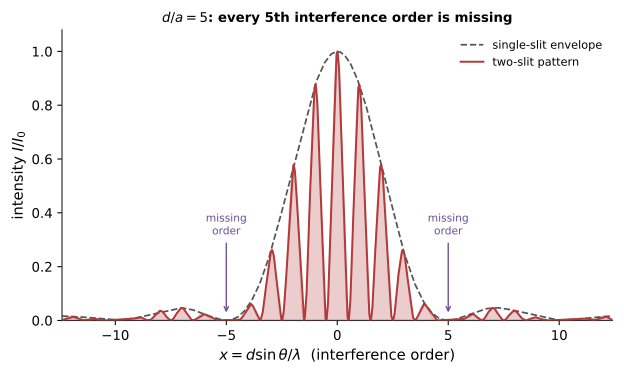
The two-slit interference fringes, a rapid cosine-squared oscillation, are modulated by the slower single-slit sinc-squared envelope; where the envelope hits zero, an interference maximum is suppressed, producing a missing order. — Figure 4.1:The two-slit pattern is the fringes ( $\cos^2$ , fast) times the envelope ( $\text{sinc}^2$ , slow). In this illustrative case $d/a=5$ , so the envelope’s first zeros extinguish the $m=\pm5$ interference orders. The pre-lab slit has a different, noninteger ratio.

The air wedge¶

Press two flat glass slides together and slip a thin object — a hair, a strip of foil — between them at one end. The air gap is approximately linear along the slides, and light reflected from the bottom of the top slide interferes with light reflected from the top of the bottom slide. Because the second reflection is off a medium of higher index, it acquires a $\pi$ phase shift, so dark fringes occur where the gap $t$ satisfies

2t = m\lambda .

(4.5)

Successive dark fringes are therefore separated by a gap change of $\lambda/2$ . If the wedge has length $\ell$ from the contact line to the spacer, and $N$ is the difference in dark-fringe order over that length, the spacer thickness is approximately

T = \frac{N\lambda}{2} .

(4.6)

A hair near $70\ \mu\text{m}$ gives $N\approx215$ at $650\ \text{nm}$ . Measure a smaller interval between identified dark fringes and scale by the ratio of lengths; count intervals rather than dark lines. This assumes the slides meet at a stable contact line and the hair alone sets the gap at its end. See this air-wedge derivation.

Pre-lab¶

Apparatus¶

Diode laser module, $\lambda \approx 650\ \text{nm}$ (use the value you measured in The Michelson Interferometer and the Ether Null Result if the same source, with its uncertainty)
Slit set with several $(a, d)$ combinations, and at least one “unknown”
Optical rail or meter stick, screen, and a mount for the camera
Camera with manual exposure and RAW output, aimed at a diffusing screen with a ruler in its plane; alternatively, a narrow-aperture photodiode on a calibrated translation stage. A bare sensor works only if its field covers enough fringe periods or it can be scanned.
Two microscope slides, gentle clips, a human hair, aluminum foil, and a magnifier or macro-imaging camera for the wedge; a beamsplitter if required by the approved reflected-light layout
Diffusing screen, beam blocks, tape measure; for Part E, a red LED, adjustable source slit, and a way to measure source-to-slit distance $D$

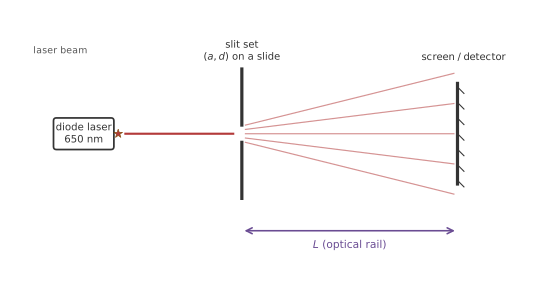
A laser beam passes through a slit set on an optical rail, and the diverging transmitted light reaches a screen or detector a distance L away. — Figure 4.2:The interference bench. Laser, slit plate, and screen or detector share a common rail so the slit-to-observation-plane distance $L$ is known. A camera may photograph the screen from outside the beam path.

Procedure¶

Before you record a pattern¶

Arrange the laser, slit plane, and observation plane in the order shown in Figure 4.2. Measure $L$ from the slit plate to the screen or sensor, not from the laser or the front of the rail.
Inventory the slit plate and copy the labeled $a$ and $d$ values into the notebook. Record which face points toward the laser so an unknown slit can be restored to the same orientation.
Level the beam through the center of the slit mount and mark the undeflected beam position on the screen. Install a beam block before moving the screen or placing a detector in the beam path.
Make a data table with slit ID, $a$ , $d$ , $L$ , exposure or detector gain, fringe positions, profile file name, and notes. Lock exposure, focus, white balance, and gain before comparing profiles.
For a camera image of the screen, take a dark frame and include a ruler in the screen plane for scale. Retake the calibration if the camera or screen moves. For a scanning photodiode, calibrate its stage positions instead.

Part A — Verifying the fringe-spacing law¶

Mount the laser, slit holder, and screen on the rail. Set $L \approx 2\ \text{m}$ . Expand the beam slightly if needed so it illuminates both slits evenly.
Choose a slit pair of known $d$ . Photograph the pattern, and also mark eleven adjacent fringe maxima on a paper screen if the envelope is wide enough. The distance between the outermost marks spans ten periods; divide it by ten. If fewer fringes are visible, record the number of intervals actually spanned and fit their positions against integer order.
Repeat for at least five values of $L$ from about $0.8\ \text{m}$ to the longest the bench allows.
Repeat for at least three values of $d$ at fixed $L$ .

[ ] Checkpoint 1. Before taking the full set, verify that your first $\Delta y$ agrees with your pre-lab prediction to about 10%. If it does not, the usual causes are a mis-measured $L$ (measure from the slit, not from the laser) or the wrong slit pair in the beam.

Part B — The full intensity profile¶

Choose the slit pair with the clearest envelope structure. Record a quantitative intensity profile:
- With a camera: image the diffusing screen with a lens from outside the beam path. Keep a ruler in the screen plane, lock focus, exposure, gain, and white balance, disable HDR and scene processing, and use RAW output if available. Take a dark frame with the beam blocked. Check that the screen and camera response are sufficiently uniform and linear for an intensity fit; otherwise use positions and envelope widths only.
- With a photodiode: mount it behind a narrow ( $\lesssim 0.1\ \text{mm}$ ) slit on a translation stage and scan in steps small compared with $\Delta y$ , logging position and voltage.
Verify that you are not saturating: the central maximum must be below the sensor’s full scale. If it is clipped, the fit will return nonsense for $a$ .
Count the central interference orders and check whether any orders align with envelope zeros. A noninteger $d/a$ need not have exactly missing orders. Write the count and any uncertainty in your notebook before fitting.

Part C — The unknown slit¶

Insert the unknown slit pair and record a profile under the same conditions. You will report $d$ and $a$ for it with uncertainties.

Part D — The air wedge¶

Clean two slides. Lay a single hair across one end, place the second slide on top, and clamp gently enough to avoid breaking glass or flattening the hair. Identify the contact line at the other end.
Illuminate at near-normal incidence with an expanded beam using the approved reflected-light layout. Block all specular reflections outside the imaging path. Image the wedge plane with a magnifier or macro camera; an un-imaged distant screen may blur the localized fringes. If the wedge contrast is inadequate, document the limitation and use the micrometer value as a separate measurement, not as a fabricated wedge result.
Measure $\ell$ from contact line to hair. On the wedge image, choose two identified dark fringes separated by a measured distance $\Delta x$ and count the intervals $\Delta m$ between them. Record image scale and uncertainty in contact and hair positions.
Measure the hair with a micrometer as an independent check.

Part E — Coherence¶

With the instructor’s source layout, replace the laser with a red LED behind an adjustable source slit at measured distance $D$ from the double slit. Start narrow enough to illuminate both slits with usable contrast, then increase source width $w$ while holding brightness settings fixed.
Record visibility or a detection limit versus $w$ . If no fringes are resolved even at the narrowest setting, document the illumination and sensitivity limit instead of claiming a coherence threshold.

Analysis¶

Fringe spacing¶

Fit $\Delta y$ against $L$ at fixed $d$ ; the slope is $\lambda/d$ . Then fit $\Delta y$ against $1/d$ at fixed $L$ ; the slope is $\lambda L$ . Multiply the first slope by its known $d$ and divide the second by its known $L$ to obtain two estimates of $\lambda$ . Account for shared calibration and distance errors when comparing them.

The full profile¶

Convert image pixels to positions $y$ in the screen plane using the ruler image, or use calibrated photodiode-stage positions. Subtract the dark frame or detector offset. Fit (4.3) with $a$ , $d$ , $I_0$ , a center offset, and a remaining background term free only if your detector response is linear enough to support an intensity fit. The simple model also assumes roughly equal illumination of the slits.

import numpy as np
from scipy.optimize import curve_fit

def two_slit(y, I0, a, d, y0, bg):
    """y in meters on the screen; small-angle sin(theta) ~ (y - y0)/L."""
    s     = (y - y0) / L                       # L defined outside, in meters
    alpha = np.pi * a * s / lam
    delta = np.pi * d * s / lam
    env   = np.sinc(alpha / np.pi) ** 2        # np.sinc(x) = sin(pi x)/(pi x)
    return I0 * env * np.cos(delta) ** 2 + bg

p0 = [prof.max() - prof.min(), 40e-6, 250e-6,
      y[np.argmax(prof)], prof.min()]
popt, pcov = curve_fit(two_slit, y, prof, p0=p0, sigma=sprof,
                       absolute_sigma=True)

Here L and lam are your measured screen distance and wavelength in meters; y, prof, and sprof are calibrated position, linear-response intensity, and its standard uncertainty. Use absolute_sigma=True only when sprof contains defensible absolute standard uncertainties. The starting guess matters: an oscillatory fit can settle into a local minimum one fringe over. Seed $d$ from Part A and $a$ from the envelope width, then inspect the residuals and fitted values. If only a processed phone image is available, use fringe positions for $d$ and envelope-zero positions for $a$ , with calibration and position uncertainties, rather than fitting pixel brightness as physical intensity.

Propagate to $d$ and $a$ from the covariance matrix, and include the uncertainty in $\lambda$ and $L$ — both enter multiplicatively.

The wedge¶

For a sub-length $\Delta x$ spanning $\Delta m$ dark-fringe intervals, use $T\approx(\Delta m\lambda/2)(\ell/\Delta x)$ at near-normal incidence. Propagate uncertainty from fringe identification, $\Delta x$ , $\ell$ , and $\lambda$ ; repeat on several image intervals to test wedge linearity. Include uncertainty from the contact line and hair position. Compare with the micrometer reading using a standardized discrepancy only when both uncertainties are defensible.

Post-lab questions¶

Going further¶

White-light fringes. With a broadband source and a compensated interferometer, fringes appear only within a coherence length of zero path difference — a few micrometres. Finding them is fiddly and is the standard technique for locating zero-order in an interferometer, used in optical coherence tomography.
Newton’s rings. A plano-convex lens on a flat gives circular fringes whose radii go approximately as $\sqrt{m}$ ; fitting their squared radii can estimate the lens’s radius of curvature. Accuracy depends on the contact gap, image scale, and how well the rings are localized.
Lloyd’s mirror. A single slit and a grazing-incidence mirror produce two-source interference from one source, with the mirror image acting as the second slit — and the fringe at the mirror surface is dark, not bright, which is a direct measurement of the $\pi$ phase shift on reflection.