Experiment 9 — Eigenmodes, Degeneracy, and Nodal Patterns¶
Objectives¶
By the end of this experiment you should be able to:
Measure resonances of a three-dimensional cavity and assign candidate quantum numbers where peaks are resolved.
Predict the splitting of a symmetry-related pair when one of two equal cavity dimensions changes, and compare it with observation.
Compare detected resonance peaks with a model count that includes degeneracy and missing or unresolved modes.
Distinguish plate nodal lines from cavity pressure nodes and hydrogenic wavefunction nodes.
Textbook connection¶
Read §9.1–9.4. The particle in a three-dimensional box is the first genuinely three-dimensional quantum problem in the book. Separable spatial modes and symmetry-related degeneracies have an acoustic analog, although the wall conditions and frequency–energy relations differ.
The Helmholtz equation for a sound wave in a rigid cavity,
is the same equation as the time-independent Schrödinger equation for a free particle in a box,
with the identification . The boundary conditions differ — a rigid wall forces while an infinite potential wall forces . Acoustic mode indices may include zero and quantum box indices may not. Their leading large-wavenumber count has the same geometric form; their low modes and boundary corrections differ.
Theory¶
Modes of a rectangular cavity¶
For a rigid-walled box of dimensions , the resonant frequencies are
(with not all zero), where is the speed of sound. The quantum counterpart, with walls, is
Same sum of squares; the frequency goes as its square root while the energy goes as the sum itself, because for a massive particle and for a wave in a non-dispersive medium. Keeping that distinction straight is one of the things this experiment is for.
Degeneracy and symmetry¶
If two dimensions are equal, say , then and have the same frequency: a symmetry-related degeneracy. Changing one of those two lengths splits the pair. A cube has larger permutation degeneracies; some unrelated triples can also share a sum of squares without being related by a symmetry.
For small detuning, the pair’s frequency difference grows approximately linearly with the changed length. This illustrates symmetry breaking, but it is not a quantitative Zeeman model: a magnetic field couples to angular momentum, whereas the cavity perturbation changes a boundary.
Density of states¶
Count the modes with frequency below . Each mode is a lattice point in space, and the number below is the volume of the corresponding octant of an ellipsoid:
where is volume and is total wall area. This is an asymptotic, smoothed count with multiplicity for rigid-wall pressure modes, excluding the static zero-frequency mode. The positive surface term reflects the Neumann wall condition. For a box at the two terms are about 34 and 19; discrete edge and corner terms and oscillations still matter. An observed peak count is usually smaller because degenerate modes share peaks and the driver or microphone can miss modes.
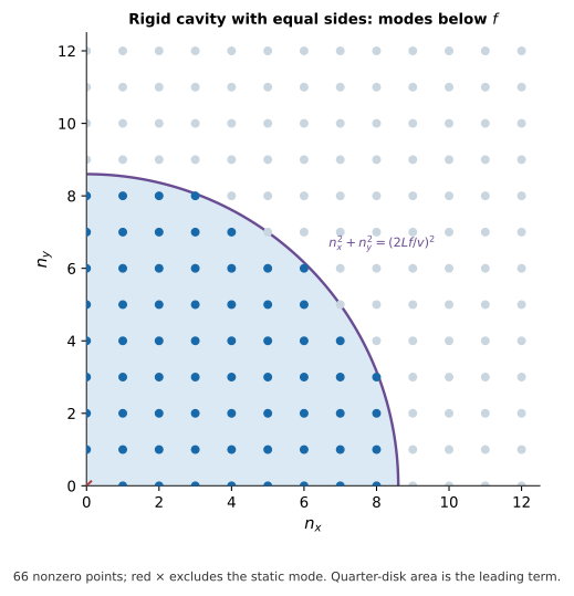
Figure 9.1:Mode counting for an equal-sided rigid cavity in two dimensions: axis points are acoustic modes, and the origin is the excluded static mode. The quarter disk area gives only the leading high-frequency count; boundary points add a lower-order correction.
Differentiating the leading term gives a density of states proportional to . The analogous electromagnetic count has two polarizations and, under classical equipartition, leads to the Rayleigh–Jeans ultraviolet catastrophe. The acoustic spectrum offers a way to inspect geometric mode counting over a limited frequency range, not a test of blackbody radiation. Real media also have finite microscopic degrees of freedom and quantum mode occupancies.
Chladni figures¶
A thin plate driven at resonance develops a bending pattern. Sand migrates from strong motion toward nodal lines. Circular-plate modes may show diametral and circular nodes, depending on drive and mounting. They give a visual analogy for angular and radial nodal structure, but a stiff plate obeys a fourth-order bending equation, unlike the second-order acoustic and Schrödinger equations. Hydrogenic angular nodes are surfaces in three dimensions, so their counts are not interchangeable with plate lines.
Pre-lab¶
Apparatus¶
Rigid rectangular cavity: a stout plywood or acrylic box, roughly internally, with two sides equal within measurement uncertainty. A small speaker and microphone near opposite corners couple well to ideal pressure modes, though real ports and driver response can still hide them. Both ports must remain inside the cavity when the partition moves. Record the exact internal dimensions and port locations.
A close-fitting, well-sealed insert or movable partition to change one of the equal dimensions while keeping both ports within the active volume
Small full-range speaker and amplifier
Electret microphone with preamp, into a sound card or a microcontroller ADC
Function generator, or a microcontroller/laptop generating a swept sine
Thin circular metal Chladni plate with a documented mount and an off-center mechanical drive or edge bow so non-axisymmetric modes can be excited; fine sand or salt
Thermometer (the speed of sound depends on temperature)
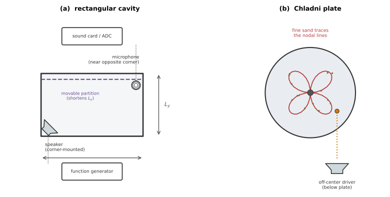
Figure 9.2:Two different standing-wave systems. (a) A swept sine drives the rectangular cavity while a corner microphone records its pressure response. (b) Sand on a Chladni plate collects near bending-mode nodal lines; the pattern is illustrative, not a calculated plate eigenfunction.
Procedure¶
Before you sweep¶
Use Figure 9.2 to distinguish the rectangular acoustic cavity from the circular Chladni plate; they are two analog systems measured with different drivers and should have separate notebook tables.
Measure internal cavity dimensions at three locations along each axis and record the mean and spread. Photograph or sketch the speaker and microphone locations, since coupling can hide modes even when their frequencies are unchanged.
Check the microphone and drive-reference channels, then close and seal every removable panel. Record sample rate, sweep rate, drive amplitude, microphone gain, and room temperature. Keep gain and drive below clipping.
Predict and tabulate the first ten mode triples before sweeping. Group equal predictions and add columns for observed peak, linewidth, candidate triples, residual, and confidence in the assignment.
For the Chladni plate, start with a very thin, even sand layer and low drive amplitude. Increase amplitude only enough to move the grains; excessive drive mixes modes and throws sand from the plate.
Part A — The mode spectrum¶
Measure , , to the inside faces, with uncertainties. Measure the air temperature.
Drive the speaker with a slow logarithmic sweep from to and record the microphone signal.
Compute a transfer response from the microphone channel divided by the measured electrical drive reference, if available. A raw microphone spectrum can be used if the drive is demonstrably flat. Peaks are candidate modes; speaker, room, and panel resonances also appear.
For each identified peak, go back and drive at a fixed frequency, scanning finely to locate the maximum. A sweep finds the modes; a fixed-frequency scan measures them.
Record all resolved candidate peaks up to the frequency where linewidths, drive response, or signal-to-noise prevent reliable assignments. Aim for ten confident assignments; distinguish a peak from the number of mode triples it may represent.
[ ] Checkpoint 1. Before recording all twenty, assign your first resolved peaks to candidate triples and compare them with your pre-lab table. The longest-axis fundamental is expected near , but a weak or missing peak can also reflect driver, microphone, or room response; test the competing explanations.
Part B — Breaking the symmetry¶
Move the sealed partition to shorten (one of the initially equal sides) by a measured 5–, without changing the speaker or microphone settings. Re-measure the low-frequency peaks.
Track the pair initially predicted as and : shortening raises the former and leaves the latter approximately fixed. Compare the measured separation with (9.3). If the initial sides were only nearly equal, include their initial separation.
Part C — Nodal patterns¶
Mount the plate on the driver, sprinkle sand thinly, and sweep slowly upward, pausing at each frequency where the sand organizes itself.
Photograph several distinct, stable patterns with their frequencies and mount and drive positions; record how many could be reproduced.
Describe apparent nodal diameters and circles, marking ambiguous or distorted lines. Do not assign a plate mode number solely from a photograph without the plate boundary conditions and a model.
Part D — Computational¶
Plot several square-well densities from . Compare the idea of nodes with a Chladni photograph, while noting the different equation and boundary conditions.
From Chapter 9, tabulate radial and angular node counts for hydrogenic , , and states. Sketch or plot one orbital density and explain which nodal feature has no direct plate counterpart.
Analysis¶
Assigning modes and fitting¶
Assign each resolved peak one representative triple or a set of unresolved candidate triples from (9.3). Count a peak once in a fit even when it represents degenerate modes; repeated entries would give one measurement excess weight. Hold the independently measured internal dimensions fixed and fit the sound speed:
import numpy as np
from scipy.optimize import curve_fit

n = np.array([[1,0,0], [0,1,0], [1,1,0], ...])  # one row per resolved peak
f = np.array([...])                             # measured frequencies, Hz
sf = np.array([...])                            # absolute frequency errors
L = np.array([Lx, Ly, Lz])                       # independently measured, m

def modes(n, v):
    return 0.5 * v * np.sqrt(((n / L) ** 2).sum(axis=1))

popt, pcov = curve_fit(modes, n, f, p0=[343.0],
                       sigma=sf, absolute_sigma=True)
v_fit, sv_fit = popt[0], np.sqrt(pcov[0, 0])
residual = f - modes(n, v_fit)
Here are the measured inside dimensions. The covariance uncertainty on is conditional on those dimensions, assignments, and the ideal-cavity model. Refit using plausible dimensions to assess geometric sensitivity, and inspect residuals for systematic shifts. Compare with for approximate dry-air speed at temperature in °C; humidity and gas composition also matter.
Do not fit and all three lengths as unrestricted parameters from frequencies alone: multiplying all four by the same factor leaves (9.3) unchanged. The data determine the three ratios , not an absolute length and speed separately. As a cross-check, use resolved axial fundamentals to infer length ratios and compare them with ruler measurements.
Degeneracy splitting¶
Plot the and peak frequencies against . For a small change with other conditions fixed, while . Compare the measured change in separation with this prediction and resolve whether the initial pair was already split. If the peaks overlap within their linewidths, report a bound on splitting rather than claiming two measured frequencies.
Density of states¶
Enumerate (9.3) through the measured frequency range, retaining one entry per triple and excluding . Plot its exact staircase count, the leading and two-term smooth approximations in (9.5), and the observed distinct-peak count separately. Their differences reveal degeneracy, unresolved linewidths, and weak coupling; the observed curve is not a complete density-of-states measurement. For the two-term smooth model with positive , its local log-slope lies between 2 and 3, not above 3. A power-law fit to a short discrete spectrum need not recover that smooth slope.
Post-lab questions¶
Going further¶
The cubic box. A box with all three dimensions equal has permutation degeneracies. It also has coincidences not related by exchanging axes: and both have a sum of squares of 27. Contrast such a numerical coincidence with hydrogen’s additional Coulomb-specific degeneracy, which has a hidden symmetry.
A cylindrical cavity. Its acoustic pressure modes involve Bessel-function conditions in the circular cross section. A circular plate also has angular separation and Bessel-related functions, but its bending equation and boundary conditions give different eigenvalues.
Damping and linewidth. Measure the full width at half maximum of an isolated power resonance and the free energy-decay time after stopping the drive. For a single weakly damped Lorentzian mode, . State the linewidth and decay-time definitions: this is a classical Fourier/damping relation, not a measurement of a quantum uncertainty principle.