The Balmer Series and the Rydberg Constant

Experiment 10 — The Balmer Series and the Rydberg Constant¶

Objectives¶

By the end of this experiment you should be able to:

Calibrate a spectrometer against known lines and assess prediction uncertainty with residuals and independent checks.
Measure the visible hydrogen emission wavelengths and assign them to transitions.
Extract the hydrogen Rydberg constant from a linear fit and compare it with the accepted value at the level of your uncertainty.
Explain why the hydrogen spectrum was the decisive test of the Bohr model and remains the reference case for atomic structure.

Textbook connection¶

Read §10.1–10.5. In the nonrelativistic Coulomb model, the Bohr and Schrödinger treatments both give approximately

E_n = -\frac{13.6\ \text{eV}}{n^2} ,

(10.1)

and the transitions among these levels are the spectrum you will measure. The Balmer series — transitions down to $n = 2$ — is the part that happens to fall in the visible, which is why a formula fitted to it in 1885 preceded any theory of atomic structure by nearly thirty years.

Theory¶

The Rydberg formula¶

Transitions from level $n_i$ to level $n_f$ emit photons with

\frac{1}{\lambda} = R_{\text{H}}\left(\frac{1}{n_f^2} - \frac{1}{n_i^2}\right) .

(10.2)

For the Balmer series $n_f = 2$ , and the visible lines are

Representative observed Balmer line centers in standard air (NIST compilation, Table 10); fine-structure components and their blends can shift a reported center

Line	Transition	Observed $\lambda$ (air, nm)	Color
H $\alpha$	$3 \to 2$	656.279	deep red
H $\beta$	$4 \to 2$	486.135	cyan
H $\gamma$	$5 \to 2$	434.047	blue-violet
H $\delta$	$6 \to 2$	410.174	violet, faint

Rearranged, (10.2) says that a plot of $1/\lambda_{\rm vac}$ against $(1/4 - 1/n_i^2)$ is a straight line through the origin with slope $R_{\text{H}}$ . That is the fit you will do, using every measurable line at once rather than averaging separate estimates. It is a leading-order model: the tabulated observed centers need not agree with its predictions to their last quoted decimal place.

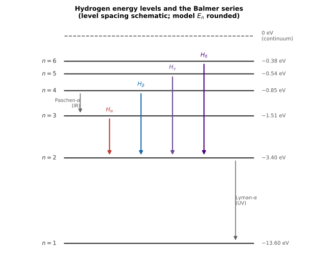
Hydrogen energy levels from n=1 to the continuum, with the four Balmer transitions from n=3,4,5,6 down to n=2 marked in color, and one representative Lyman and Paschen transition shown in gray for context. — Figure 10.1:The Balmer series is one column in a larger structure: every visible line you measure is a transition landing on $n=2$ ; Lyman lines land on $n=1$ (in the UV) and Paschen lines on $n=3$ (in the IR) — neither visible to the eye, which is why Balmer’s formula came first.

Which Rydberg constant?¶

Two constants appear in the literature and they are not the same:

R_\infty = \frac{m_e e^4}{8\varepsilon_0^2 h^3 c} = 1.0973731568\times10^{7}\ \text{m}^{-1}

(10.3)

is the value for an infinitely heavy nucleus, and

R_{\text{H}} = \frac{R_\infty}{1 + m_e/M_p} = 1.0967758\times10^{7}\ \text{m}^{-1}

(10.4)

is the value for hydrogen, corrected for the finite proton mass through the reduced mass $\mu = m_eM_p/(m_e + M_p)$ . They differ by about $0.054\%$ . Separating them requires an uncertainty budget smaller than that difference, including calibration, air conversion, and the limits of the simple line-center model. A small fit error alone does not establish a measurement of the proton-to-electron mass ratio. State whether your total uncertainty can distinguish the two constants.

Air versus vacuum¶

Wavelengths measured in air are shorter than in vacuum by the refractive index of air, $n \approx 1.00027$ in the visible — a $0.027\%$ effect, comparable to the reduced-mass correction above. Tabulated “air wavelengths” (the values in the table above) already include it. Be explicit about which convention you are using, or you will chase a systematic of exactly the size of the physics you are trying to see. The refractive index varies with wavelength and ambient conditions. Use a wavelength-dependent standard-air conversion for a precise comparison, or include the approximation in your uncertainty budget.

Pre-lab¶

Apparatus¶

Hydrogen discharge tube with a high-voltage power supply
Mercury and helium discharge tubes, for calibration
Either: a calibrated grating spectrometer with a vernier circle, the reflective-grating Thorlabs EDU-SPEB2 visual kit, or a compact USB spectrometer with a fiber input. A detector scan needs suitable scanning hardware, such as the EDU-SPEBCT1 extension or a USB spectrometer.
Entrance slit of adjustable width
Thermometer and barometer, if you intend to make the air-index correction yourself

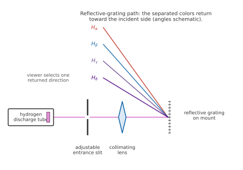
Light from a hydrogen discharge tube passes through an adjustable entrance slit and a collimating lens, then reflects from a grating. Four Balmer colors return on the incident side at different angles toward a movable viewer. — Figure 10.2:Reflective-grating spectrometer, shown schematically. Collimated light from the entrance slit reaches the grating; each Balmer line returns at a different angle on the incident side. Use the actual instrument geometry and its angle zero for conversion to wavelength.

Procedure¶

Before you calibrate¶

Identify the entrance slit, collimator, grating, telescope or detector, and angular zero in Figure 10.2. Record the grating type, line spacing, order, incidence angle, and angle convention for the actual setup; the drawing only indicates dispersion.
Allow each discharge lamp and the detector to warm up for the manufacturer’s recommended time. Keep high-voltage lamp leads covered and switch the supply off before changing tubes.
Focus the entrance slit first, then the collimator, and finally the detector or telescope. Record slit width, focus, and fiber placement; changes to any of them require a calibration check.
Prepare a calibration table containing lamp, accepted wavelength, measured angle or pixel, approach direction, trial, residual, and uncertainty. Keep a separate table for unassigned features so they are not silently discarded.
Choose a consistent line-center rule—centroid, fitted peak, or midpoint of a symmetric visual line—and use it for both calibration and Balmer lines.

Part A — Calibration¶

Set up the spectrometer and focus it on the entrance slit. Narrow the slit until the lines are sharp; note that narrowing further past this point costs intensity without improving resolution.
With the mercury lamp, measure the positions of several resolved known lines across the available span. Resolve the close 577/579 nm pair before counting them separately. Record the line-center rule and repeats.
Calibrate with the geometry of your instrument. For a normal-incidence transmission grating, $d\sin\theta=m\lambda$ . A reflective grating at oblique incidence needs both incidence and diffraction angles with a stated signed-angle convention; the normal-incidence formula does not apply to it. For a USB spectrometer, fit a justified low-order pixel-to- wavelength relation. Check the actual lamp or detector wavelength range.
Check the fit and its prediction uncertainty. Plot signed residuals versus wavelength. Estimate line-center repeatability, uncertainty in the fitted calibration, and any model mismatch separately. Residual RMS alone is not a systematic uncertainty for each subsequent line.
Use the helium line near 667.8 nm to extend calibration beyond H $\alpha$ or reserve it as an independent extrapolation check. Do not use the same line for both roles. Other held-out lines can check the blue range.

[ ] Checkpoint 1. Show the instructor your calibration fit, residuals, and a held-out check. Resolve any gross misidentification or drift before measuring hydrogen; document the achieved calibration accuracy.

Part B — The Balmer lines¶

Replace the calibration lamp with the hydrogen tube using the approved shutdown procedure. Recheck slit illumination and an accessible reference line after the swap; if the slit, grating, or fiber moved, recalibrate.
Locate H $\alpha$ through H $\delta$ where resolved and measurable. Measure each usable line at least five times. On a vernier instrument, approach from alternating directions to expose backlash.
H $\delta$ is faint. If you widen the slit, repeat nearby blue calibration lines at that width and record any center shift or blending. Do not invent a center for an unresolved line; three well-measured lines can still fit the one-parameter model.
Watch for molecular hydrogen bands — the tube emits from H $_2$ as well as H, creating extra spectral features that are not the Balmer series. The Balmer lines are sharp and bright; the molecular bands are broad and clustered. Note in your notebook which features you rejected and why.

Part C — Re-calibration¶

Return to calibration lamps and re-measure at least one blue and one red line, preferably bracketing the measured span. Treat a shift as evidence of drift and include its effect in the uncertainty budget.

Analysis¶

Wavelengths¶

Apply the calibration to each measured position. Combine repeat scatter with calibration prediction uncertainty, checks for drift and model mismatch, and the air-index conversion. A common calibration error correlates the reported wavelengths. Quote each $\lambda$ with an uncertainty, and compare each with the observed line centers individually before fitting. At the few-pm level, include the difference between observed blended centers and the simple Rydberg model in the interpretation.

The Rydberg constant¶

import numpy as np
from scipy.optimize import curve_fit

ni = np.array([...])                  # upper n for each usable line, >= 3 lines
lam = np.array([...])                 # measured VACUUM wavelengths, meters
Clam = np.array([...])                # full wavelength covariance, m^2

x   = 0.25 - 1.0 / ni**2
y   = 1.0 / lam
Cy  = Clam / np.outer(lam**2, lam**2)  # propagate 1/lambda

popt, pcov = curve_fit(lambda x, R: R * x, x, y,
                       sigma=Cy, absolute_sigma=True)
R, sR = popt[0], np.sqrt(pcov[0, 0])
print(f"R_H = {R:.7g} +/- {sR:.2g} 1/m")

Convert measured air wavelengths to vacuum first ( $\lambda_{\text{vac}} = n_{\text{air}}\lambda_{\text{air}}$ ). Use a wavelength-dependent air index at the recorded conditions if your precision requires it. The $R_{\text{H}}$ model uses vacuum wavelengths. Build Clam from repeat variability and calibration-parameter covariance; include shared terms off the diagonal. Test additional plausible drift or line-center models separately if their effects cannot be represented by this matrix.

Fit with the intercept forced to zero, then use a free-intercept fit as a diagnostic. A nonzero intercept can arise from calibration, blending, or model limitations; it is not by itself a unique diagnosis.

The reduced-mass question¶

Only if the total uncertainty and model checks support distinguishing $R_{\text{H}}$ from $R_\infty$ , explore

\frac{m_e}{M_p} = \frac{R_\infty}{R_{\text{H,measured}}} - 1

(10.5)

and compare with $1/1836.15$ . Propagate the uncertainty in your measured $R_{\text{H}}$ and state the assumptions behind this leading-order relation. Otherwise report the bound your data place on the difference and explain why they do not determine the mass ratio.

Post-lab questions¶

Going further¶

The deuterium isotope shift. A deuterium lamp’s H $\alpha$ sits $0.18\ \text{nm}$ from hydrogen’s, because the reduced mass differs. That requires $\lambda/\Delta\lambda \approx 3700$ merely to separate the ideal centers; line width and calibration must also support the measurement. The isotope shift supplied evidence in the 1931–32 discovery of deuterium.
Sodium as a contrast case. Measure the sodium doublet on the same instrument, and note that no simple Rydberg formula fits it. Explaining why is Week 11.
Balmer in absorption. The same lines appear as dark lines in the spectra of A-type stars. A small telescope with a grating in front of the objective will show them, and identifying the Balmer series in Vega with the calibration you built today is one of the more satisfying evenings available to an undergraduate.