Experiment 13 — Counting Statistics, Half-Life, and Gamma Attenuation¶
Objectives¶
By the end of this experiment you should be able to:
Test whether repeated counts are consistent with a Poisson model, and state when is a useful uncertainty estimate.
Distinguish the Poisson and Gaussian regimes and know when each applies.
Measure a short half-life from interval counts with a Poisson fit.
Estimate a gamma attenuation coefficient and compare the result with a narrow-beam reference after checking the measurement geometry.
Textbook connection¶
Read §13.3–13.6. This experiment is the practical foundation for everything in
nuclear and particle physics: essentially every measurement in the field is a
counting measurement. Its uncertainty includes random counts, background
subtraction, dead time, geometry, and calibration. This experiment explains
when the sqrt(N) approximation used since Week 3 is appropriate.
Theory¶
Why decay is Poisson¶
Each nucleus in a sample has the same probability of decaying in any short interval , independently of its age and of every other nucleus. For a large number of nuclei each with a small probability of decaying, the number observed in a fixed interval follows the Poisson distribution
whose mean and variance are both . Hence the standard deviation is . For sufficiently many counts, a single observation gives the approximate standard uncertainty . In an ideal gross count with negligible background and dead time, the relative uncertainty is then : 1% needs about 104 counts and 0.1% needs 106. Subtracting an independently measured background adds its counting variance.
For the Poisson distribution is well approximated by a Gaussian of mean and standard deviation . Below that it is visibly asymmetric, and for small the difference matters: at the estimator is plainly wrong, and one must use a proper confidence interval instead. You will observe both regimes today.
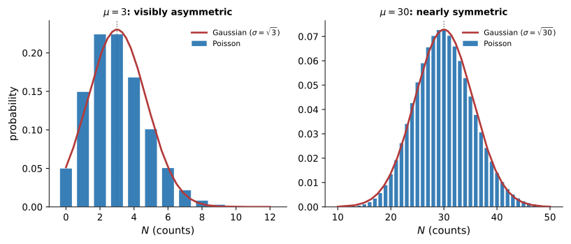
Figure 13.1:The same law, two regimes. At the Poisson distribution is visibly skewed and the Gaussian density is poor near ; at their shapes are close. The bars show probabilities and the line is a continuous density.
Decay law¶
The measured count rate is proportional to the activity , so the rate obeys the same exponential.
The isotope generator¶
Cs () feeds metastable Ba, which has and emits a gamma in its de-excitation. A licensed generator can retain the caesium while barium is eluted under its approved procedure. Do not assume perfect parent retention: the instructor checks for long-lived Cs breakthrough and controls the eluate and waste.
Gamma attenuation¶
A narrow beam of monoenergetic gammas through an absorber of thickness follows
where is the linear attenuation coefficient. Each interaction removes a primary gamma from the unscattered beam, producing an exponential primary transmission. A GM counter has no energy resolution and can also count scattered photons that reach it.
At the dominant mechanism in light materials is Compton scattering, which scales roughly with electron density and therefore with — nearly constant across the periodic table. In lead, the higher- photoelectric contribution is also significant. The NIST mass attenuation coefficients at are about for lead and for aluminum, giving narrow-beam half-value layers of roughly and respectively. Look these up yourself in XCOM rather than taking them from here.
Pre-lab¶
Apparatus¶
GM tube, counter/timer with programmable repeat runs, and HV supply
Cs/Ba isotope generator, eluting solution, planchets, gloves, tray
Sealed Cs check source for the 662 keV attenuation measurement
Lead sheets (1–) and the available aluminum absorber set
Collimator, if available
Stopwatch; the source log
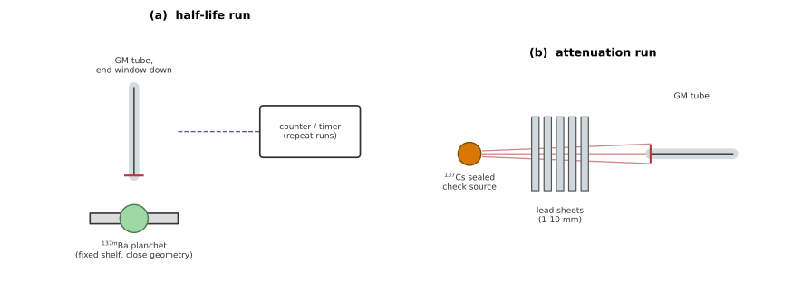
Figure 13.2:Two fixed geometries. (a) The short-lived Ba planchet counted at close, unchanging range for the half-life run. (b) A long-lived check source counted through increasing lead thickness for the attenuation run.
Procedure¶
Before you start the timed runs¶
Identify the two independent geometries in Figure 13.2: the generator eluate directly beneath the GM tube for half-life and the sealed source–absorber–tube line for attenuation. Record dimensions for each and do not transfer distances from the schematic.
Verify the counter clock and repeat mode with ten short test intervals. Make sure it stores each interval separately, including its start and end times and whether the duration is wall time or corrected live time.
Prepare three machine-readable tables: repeated counts, decay time series, and attenuation. Include raw counts, start time, live time, source, absorber, geometry, high voltage, and run ID in every applicable row.
Measure background in the geometry used for each part. Record raw background counts and duration; do not enter a pre-subtracted rate into the primary data file. Background is part of the fitted count model.
Plan source handling before elution, including who starts the counter and who records the elution time. Rehearse once without activity so the first decay point is not lost to confusion.
Part A — The statistics of counting¶
Set the operating voltage from the plateau, as in Relativistic Electrons from Beta Decay.
Place a long-lived source so that you get an average of about 3 counts per one-second interval, including background. Take at least 300 one-second runs. Use the counter’s repeat mode; do not do this with a stopwatch.
Move the source (or increase the interval) so that you get an average of about 30 counts per interval. Take another 300 runs.
Take 300 runs of pure background at the same interval. Check that the mean does not drift during either series; a changing rate is not a single stationary Poisson process.
[ ] Checkpoint 1. Show the instructor your two mean counts and confirm they are near 3 and 30 before committing to the full runs.
Part B — Half-life of Ba¶
Set the counter to take at least 90 consecutive runs, recording every interval. Aim for an early observed rate below about if the nonparalyzable dead time is ; this limits the lost-count fraction to about 1%. Verify the actual detector dead time and adjust the approved source geometry before elution.
Elute the generator onto a planchet, put it under the detector at a fixed geometry, and start counting. Record the elution time.
Let the run continue for at least — about six half-lives, over which the rate falls by a factor of about 60.
This may not reach background: a hypothetical sample starting at remains near after 15 minutes and needs about 30 minutes to approach a background. Measure background before elution and after the run. Fit it jointly with the decay data and background count, so its finite precision is included. Investigate any apparent persistent activity as possible breakthrough.
Do not move the sample or the detector during the run.
If time allows, elute a second sample and repeat. Two independent decay curves is a much better basis for a claimed uncertainty than one.
Part C — Gamma attenuation¶
Remove and control the eluate as directed, then use a sealed Cs source at a fixed geometry. Record source, absorber, and detector apertures and separations; collimate if the approved setup allows it.
Measure lead at several thicknesses spanning as much of the available transmission range as practical. Increase counting time as the rate falls, aiming for comparable uncertainty in net rates. Record each sheet’s thickness and the stack order.
Repeat with aluminum over the thickness available. Report the actual number of half-value layers covered rather than assuming the kit spans four.
Measure background with the source removed in the same detector and absorber geometry, including a check near each end of the series.
Analysis¶
Testing the Poisson hypothesis¶
import numpy as np
from scipy.stats import poisson, norm

counts = np.array([...])                 # 300 equal-duration gross counts
mu     = counts.mean()
var    = counts.var(ddof=1)
print(f"mean = {mu:.3f},  variance = {var:.3f},  ratio = {var/mu:.3f}")

# Include every observation and a model tail in the last bin.
kmax = max(counts.max(), int(poisson.ppf(0.9999, mu)))
k    = np.arange(kmax + 1)
obs  = np.bincount(counts, minlength=k.size)
exp_p = counts.size * poisson.pmf(k, mu)
exp_p[-1] = counts.size * poisson.sf(kmax - 1, mu)

# Continuity-corrected Gaussian probabilities for integer-count bins.
exp_g = counts.size * (norm.cdf(k + 0.5, mu, np.sqrt(mu))
                       - norm.cdf(k - 0.5, mu, np.sqrt(mu)))
exp_g[0] = counts.size * norm.cdf(0.5, mu, np.sqrt(mu))
exp_g[-1] = counts.size * norm.sf(kmax - 0.5, mu, np.sqrt(mu))
For a Poisson process the variance-to-mean ratio should be 1. Report it with an uncertainty — for samples, the ratio has a standard deviation of approximately under the stationary Poisson model. Combine adjacent tail bins until each model’s expected count is at least about 5, then compute . With final bins and one mean estimated from the data, use approximately degrees of freedom. Document the bins; the Gaussian approximation includes its negative tail in the zero-count bin.
At the Gaussian approximation has a visibly different shape; 300 trials may or may not reject it at a chosen significance level. At the two models are close. Present both comparisons with the observed histogram, and interpret a non-rejection as limited evidence, not proof that a model is exact.
The half-life¶
import numpy as np
from scipy.optimize import minimize
from scipy.special import xlogy

t0 = np.array([...])       # interval starts, seconds since elution
t1 = np.array([...])       # interval ends, seconds since elution
N = np.array([...])        # raw gross counts in those intervals
B, TB = ..., ...           # separate background count and duration (s)
dt = t1 - t0

def expected(logpars):
    r0, lam, bg = np.exp(logpars)  # source rate at elution, decay, background
    signal = r0 * np.exp(-lam * t0) * (-np.expm1(-lam * dt)) / lam
    return signal + bg * dt, bg

def nll(logpars):
    mean, bg = expected(logpars)
    return np.sum(mean - xlogy(N, mean)) + bg * TB - xlogy(B, bg * TB)

guess = np.log([max(N[0] / dt[0], 0.1), np.log(2) / 153.12,
                max(B / TB, 0.001)])
fit = minimize(nll, guess)
if not fit.success:
    raise RuntimeError(fit.message)
lam = np.exp(fit.x[1])
T12 = np.log(2) / lam
The fit uses the expected count integrated over each real interval and includes the separate background measurement in the same likelihood. Obtain a half-life interval by profiling the likelihood or by simulating new count series and background counts from the fitted model and refitting. Check the following:
Keep the raw counts. Subtracting background before a Poisson fit or weighting each point by fails at small .
Keep real time stamps. For equal interval widths, replacing each integral by a midpoint value changes the fitted amplitude, not the exponential slope. For a 10 s interval at this half-life the integrated value differs from the midpoint approximation by only about 0.009%. Irregular or missed intervals still need their actual bounds.
Check dead time. At low rates the Poisson model above is suitable. If the measured early dead-time loss is material, incorporate a calibrated detector model or repeat at greater source–detector distance; a naive correction to counts does not preserve Poisson uncertainties.
Plot count residuals against time. Early or late patterns can suggest dead time, geometry changes, background error, or parent breakthrough; investigate with controls rather than assigning a cause from the shape alone.
Attenuation¶
Fit gross interval counts with a source term proportional to plus measured background, using a Poisson likelihood and each point’s acquisition time. Check dead time at the thinnest absorber and propagate thickness and density uncertainty when calculating and . Compare the material values with NIST XCOM at the same energy. If the detector accepts scattered photons, label the fitted value an effective attenuation coefficient; agreement or disagreement alone cannot establish an interaction mechanism.
Post-lab questions¶
Going further¶
The interval distribution. The times between successive counts in a Poisson process follow an exponential distribution. Logging individual event timestamps with a microcontroller and histogramming the intervals shows this directly, and the deficit of very short intervals is a clean, independent measurement of the detector’s dead time.
Two-source dead-time measurement. Count source A, source B, and both together. Because when counts are lost, the deficit can estimate after background and geometry corrections, under an explicit paralyzable or nonparalyzable detector model.
Gamma spectroscopy. A scintillator and a multichannel analyzer resolve the photopeak from the Compton continuum and edge, letting you verify the Compton formula from Chapter 6 with the same source. Compute the expected Compton edge at and look for it.