The Michelson Interferometer and the Ether Null Result

Experiment 1 — The Michelson Interferometer and the Ether Null Result¶

Objectives¶

By the end of this experiment you should be able to:

Align a Michelson interferometer and explain the function of each optic in it.
Relate a counted number of fringe transitions to a mirror displacement, and use the relation to measure an optical wavelength.
Estimate the smallest fringe shift your apparatus can detect, and convert that threshold into the smallest hypothetical ether drift it could detect under the simple stationary-ether model.
Explain how the Michelson–Morley null result constrained that model and why simple complete-drag proposals faced other observations.

Textbook connection¶

Read §1.3–1.5 of Chapter 1 before the period. The interferometer you will align is the same instrument, in miniature, that Michelson and Morley floated on a bed of mercury in 1887. The difference between what they were trying to detect and what you can detect on a laboratory bench in three hours is itself worth understanding, and is the subject of the analysis below.

Theory¶

Fringes from a path difference¶

A Michelson interferometer splits a beam in two at a beamsplitter, sends the halves down two perpendicular arms of lengths $L_1$ and $L_2$ , and recombines them. Each beam traverses its arm twice, so the optical path difference is

\Delta = 2(L_1 - L_2).

(1.1)

Constructive interference at the output occurs when $\Delta = m\lambda$ for integer $m$ . Translating one mirror by a distance $d$ changes $\Delta$ by $2d$ , and the number of bright fringes $N$ that sweep past a fixed point in the output pattern is

N = \frac{2d}{\lambda} \qquad\Longleftrightarrow\qquad \lambda = \frac{2d}{N}.

(1.2)

This is the entire measurement. Its beauty is that it converts a wavelength — a sub-micrometre quantity you cannot rule off — into a count, which needs careful tracking but no length calibration, and a mirror displacement, which you can measure with a micrometer. The factor of two is the most commonly dropped quantity in this experiment; it is there because light traverses the arm both ways.

Why the fringes are circles¶

With a slightly diverging beam and mirrors that are accurately perpendicular, rays leaving the source at angle $\theta$ to the axis acquire path difference $\Delta = 2d\cos\theta$ , so the interference condition depends only on $\theta$ : the pattern is a set of concentric circles, and translating the mirror makes them swallow into, or boil out of, the center. If the mirrors are not quite perpendicular, the fringes become straight and parallel — still usable, and in fact easier to count. Either pattern obeys (1.2) at the center of the field.

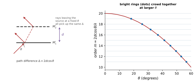
Two parallel mirror planes separated by d, with a ray leaving the source at angle theta picking up path difference 2d cos theta; a plot of the fringe order against theta shows the bright rings crowding together at larger angles. — Figure 1.1:Left: unfolding the interferometer into two parallel mirror planes $M_1'$ and $M_2'$ shows that every ray leaving the source at the *same* angle $\theta$ to the axis acquires the *same* path difference $\Delta = 2d\cos\theta$ — hence a ring, not a spot, of constant phase. Right: because $\cos\theta$ falls off faster as $\theta$ grows, successive orders $m$ crowd closer together at larger $\theta$ — the rings are not evenly spaced.

What Michelson and Morley were looking for¶

If light propagated in a medium at rest in some absolute frame, and the Earth moved through that medium at speed $v$ , the round-trip times along the two arms would differ. To first order in $(v/c)^2$ , the fringe shift on rotating the apparatus by $90°$ is

\Delta N = \frac{2L}{\lambda}\left(\frac{v}{c}\right)^{2},

(1.3)

where $L$ is the arm length (taken equal for both arms). The quadratic dependence on $v/c$ is what makes the experiment hard: for the Earth’s orbital speed $v = 30\ \text{km/s}$ , $(v/c)^2 = 10^{-8}$ , so even a meter of arm length buys only a few hundredths of a fringe.

Michelson and Morley beat this by folding the beam through multiple reflections to reach an effective $L = 11\ \text{m}$ , and by floating the whole apparatus on mercury so it could be rotated continuously while being watched. They expected a shift of about 0.4 fringes and reported less than about 0.01 fringe, under the assumptions of that model; see their 1887 paper. You will not repeat their sensitivity. You will quantify how far short of it you fall, which is the honest version of the experiment and teaches more than a rigged one would.

Pre-lab¶

Answer in your notebook before you arrive.

Apparatus¶

Michelson interferometer with micrometer-driven movable mirror — a bench instrument, or the Thorlabs EDU-MINT1 kit built on a breadboard
red HeNe laser (approximately $632.8\ \text{nm}$ in air) or a $\sim650\ \text{nm}$ diode laser module
Short-focal-length diverging lens ( $f \approx -25\ \text{mm}$ ) to expand the beam
Viewing screen or white card; optional photodiode + oscilloscope for automated counting
Beam stops; wavelength-rated laser eyewear when required by the site’s laser safety assessment
Tally counter (or the counter app on a phone)

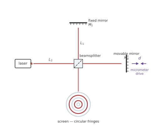
A laser beam is split at a beamsplitter into two arms, one to a fixed mirror and one to a micrometer-driven movable mirror, recombining to form circular fringes on a screen. — Figure 1.2:The Michelson interferometer. The beamsplitter sends light down two perpendicular arms; translating the movable mirror by $d$ sweeps $N = 2d/\lambda$ fringes past a point on the screen.

Procedure¶

Before you align¶

Use Figure 1.2 to identify the two arms, the fixed-mirror adjustment, and the micrometer drive. The drawing is a beam-path guide, not a scale drawing; measure both arm lengths on your own instrument.
Draw a top view of your actual setup in the notebook. Mark the beam height, every beam block, which mirror moves, and the positive micrometer direction.
Make a table with columns for run, direction of travel, initial and final micrometer readings, fringe count, and comments. Leave room for five runs.
Check that every mount is clamped, the beamsplitter is seated, and the laser terminates on a screen or block. Remove reflective jewelry before the laser is switched on.
Decide who will turn the micrometer and who will count. Do not exchange jobs during a run; stop and restart a run if either person loses the count.

Part A — Alignment¶

With the beam-expanding lens removed, send the raw laser beam into the beamsplitter. You should see two spots on the screen: one from each arm.
Adjust the tilt screws on the fixed mirror until the two spots coincide. Work on the dimmer of the two spots so you can tell which is which.
When the spots overlap, faint interference fringes may appear. If they do not, check overlap, polarization, and arm-length matching. A diode laser can have a short coherence length; equalize the arms before fine tuning.
Insert the diverging lens between the laser and the beamsplitter. The fringes should expand into a circular bullseye filling the screen.
Fine-tune the fixed-mirror tilt until the bullseye is centered and its center is as large and slow-moving as you can make it.

[ ] Checkpoint 1. Show the instructor a stable circular fringe pattern. Do not proceed with a pattern that drifts on its own faster than about one fringe per ten seconds — find the source (usually someone leaning on the table, an air current from a vent, or an unlocked mount) and fix it.

Part B — Measuring the wavelength¶

Record the micrometer reading. For the primary runs, approach both endpoints from the same direction after taking up any backlash. Reversing direction without doing this may make the micrometer reading differ from the mirror’s actual motion. Estimate that effect on your instrument rather than assuming a fixed size.
Choose a reference feature at the center of the pattern. Translate the mirror slowly and steadily, counting fringe transitions with the tally counter. Have your partner call out at every 50 counts so you can catch a miscount.
Stop at $N = 200$ (or the count you chose in Exercise 1.1) and record the final micrometer reading. [ ] Checkpoint 2. Compute $\lambda$ from your first run before you take the other four. If it is not within about 10% of $633\ \text{nm}$ , you have a factor-of-two problem or a micrometer scale problem, and it is much cheaper to find it now.
Take four more runs at a few different fringe counts. Repeat at least one count in both directions for a like-for-like backlash check; first take up backlash after each reversal. Keep direction in the data table. Do not pool direction-dependent results until you have checked and accounted for the difference.
Record the uncertainty you assign to each micrometer reading and fringe count while you are still at the bench.

Part C — Bounding the ether drift¶

Measure both arm lengths from the beamsplitter face to each mirror, with an uncertainty.
With the pattern stable, determine the smallest fringe shift you can reliably detect. Do this operationally rather than by guessing: have your partner translate the mirror by a small unknown amount, half the time by nothing at all, and see how small a real shift you can still call correctly. Ten trials is enough to establish the threshold to a factor of two.
If the instrument can be rotated on the bench (the EDU-MINT1 breadboard can be turned; a heavy bench interferometer usually cannot), rotate it through $90°$ and watch the pattern. Record any shift you see, and its uncertainty. Check for mechanical flexure with repeated rotations. A shift that follows a loose optic is not evidence for the modeled drift.

Analysis¶

Wavelength¶

For each run, $\lambda_i = 2d_i/N_i$ . Propagate the uncertainty in $d$ and, if you think a miscount is plausible, in $N$ :

\left(\frac{\sigma_\lambda}{\lambda}\right)^2 = \left(\frac{\sigma_d}{d}\right)^2 + \left(\frac{\sigma_N}{N}\right)^2 .

(1.4)

Compare the five runs by direction before combining them. Take a weighted mean only of runs whose differences are consistent with their uncertainties and whose shared calibration effects have been included. Excess scatter could come from backlash, drift, miscounts, or underestimated reading errors; investigate it rather than assigning one cause automatically. For $N=200$ and $\lambda\approx633\ \text{nm}$ , the mirror moves only about $63\ \mu\text{m}$ . A $1\ \mu\text{m}$ uncertainty on each endpoint already contributes about 2.2% to one displacement, before counting errors.

An alternative uses all compatible runs at once: plot $d$ against $N$ and fit a straight line. First allow an intercept and inspect it; only constrain the intercept to zero if the data and measurement method justify it. The slope is $\lambda/2$ .

import numpy as np
from scipy.optimize import curve_fit

N  = np.array([100, 200, 200, 400, 400])          # fringe counts
d  = np.array([...])                              # displacements, meters
sd = np.array([...])                              # uncertainty on each d, meters

line = lambda n, half_lambda, offset: half_lambda * n + offset
popt, pcov = curve_fit(line, N, d, sigma=sd, absolute_sigma=True)

lam, slam = 2 * popt[0], 2 * np.sqrt(pcov[0, 0])
print(f"offset = {popt[1]*1e6:.1f} +/- {np.sqrt(pcov[1,1])*1e6:.1f} um")
print(f"lambda = {lam*1e9:.1f} +/- {slam*1e9:.1f} nm")

Sensitivity to the modeled ether drift¶

Rearrange (1.3) for the speed corresponding to your detection threshold $\Delta N_{\min}$ :

v_{\mathrm{sens}} = c\,\sqrt{\frac{\lambda\,\Delta N_{\min}}{2L}} .

(1.5)

This is the minimum detectable speed under the simplified model, not an upper bound measured by a stationary instrument. Quote it in km/s and as a fraction of $c$ , and give a plausible range based on the uncertainty in your threshold and arm length. Compare it with the Earth’s orbital speed of $29.8\ \text{km/s}$ and the historical experiment’s sensitivity. Only a controlled rotation with a null result could support an experimental upper bound under the model, and mechanical shifts must be excluded first.

Post-lab questions¶

Going further¶

Automate the count. Put a photodiode at the center of the pattern, feed it to an oscilloscope or a microcontroller ADC, and drive the mirror with a stepper. Counting transitions in software can reduce human miscounts, but check for false triggers and missed fringes. This is the same technique that turns an interferometer into a displacement metrology instrument good to nanometres.
Measure the refractive index of air. Put an evacuable cell of length $\ell$ in one arm and count fringes as it is pumped down: $n - 1 = N\lambda/(2\ell)$ . Expect $n - 1 \approx 2.7\times10^{-4}$ at laboratory pressure. Use an appropriately rated vacuum pump and cell, and measure the pressure; the fringe count alone does not establish three-digit accuracy.
Measure the sodium doublet. With a sodium lamp instead of a laser, the fringe visibility collapses and revives as the two D lines drift in and out of phase. The mirror displacement between successive collapses gives the splitting $\Delta\lambda = \lambda^2/(2\Delta d)$ — a $0.6\ \text{nm}$ splitting measured with a micrometer, and a preview of Alkali Spectra, Screening, and the Quantum Defect.