Relativistic Electrons from Beta Decay - Modern Physics Laboratory

Experiment 3 — Relativistic Electrons from Beta Decay¶

Objectives¶

By the end of this experiment you should be able to:

Measure an absorption curve and estimate a practical range from its terminal region, while recognizing when the available absorber thickness is insufficient.
Convert a range in aluminum into a maximum kinetic energy using an empirical range–energy relation.
Compute $v/c$ for that energy both relativistically and classically, and explain why the classical answer is not merely inaccurate but impossible.
Handle counting data correctly: Poisson uncertainties, background subtraction, and dead time.

Textbook connection¶

Read §3.1–3.4. This experiment supplies the number that makes relativistic dynamics unavoidable in a first course. A beta particle from $^{90}$ Y carries up to $2.28\ \text{MeV}$ of kinetic energy — more than four times its own rest energy — and the classical expression $T = \tfrac12 mv^2$ returns a speed of about $3c$ for it. Nothing else on the bench makes the failure of Newtonian mechanics so blunt.

Theory¶

The beta spectrum and its endpoint¶

Beta decay is a three-body process: the nucleus emits an electron and an antineutrino, which share the available energy. The electron therefore emerges with a continuous spectrum of energies from zero up to a maximum $T_{\max} = Q$ , the endpoint, reached in the rare case that the neutrino takes essentially nothing. It was precisely this continuous spectrum — apparently violating energy conservation — that led Pauli to postulate the neutrino in 1930, so the shape you are measuring around today has some history in it.

After several $^{90}$ Y half-lives, an older sealed $^{90}$ Sr source contains $^{90}$ Sr/ $^{90}$ Y near secular equilibrium:

^{90}\text{Sr} \xrightarrow{\ \beta^-,\ 28.91\ \text{y}\ } {}^{90}\text{Y} \xrightarrow{\ \beta^-,\ 64.05\ \text{h}\ } {}^{90}\text{Zr\ (stable)} ,

(3.1)

with endpoints $0.546\ \text{MeV}$ and $2.28\ \text{MeV}$ respectively. The high-energy $^{90}$ Y component is the one whose range you will measure, because it is the only beta component that survives the thicker absorbers. See the evaluated strontium-90 and yttrium-90 decay data.

Absorption and range¶

Beta particles lose energy mainly through collisions and can also produce bremsstrahlung photons. The counting rate behind an absorber of mass thickness $x$ (in $\text{mg/cm}^2$ : density times physical thickness) falls as the electron spectrum is filtered. A single exponential is a rough description of part of that curve, not a law for the mixed source:

R(x) = R_0\, e^{-\mu_m x} + R_{\text{bg}} ,

(3.2)

At large thickness, the measured rate may approach a floor from background and source-related photons. The practical, or extrapolated, range $R_m$ is estimated from the terminal electron-dominated decline and its intersection with that floor on a linear rate axis. It is not the thickness at which every electron track ends, and a threshold chosen from counting noise does not define it. See the Katz–Penfold range study and the University of Texas at Arlington absorption procedure.

Mass thickness is used rather than physical thickness because energy loss per unit mass is nearly the same in all light materials — so a range quoted in $\text{mg/cm}^2$ is roughly transferable between absorber materials, which physical millimeters are not.

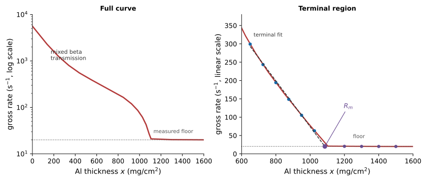
Left, a semilog plot shows a rapid fall in beta transmission and a flat background-plus-photon floor. Right, a linear-scale view of the terminal region fits its declining count rate and marks the intersection with the measured floor as practical range R_m. — Figure 3.1:Read the full curve on a log rate axis to identify the components. Estimate $R_m$ from the terminal electron-dominated decline on a linear rate axis, extrapolated to a floor measured with thicker absorbers. If the floor or the terminal decline is absent, the plot does not support an endpoint estimate.

From range to energy¶

Two standard empirical relations connect the maximum range in aluminum to the endpoint energy. Feather’s rule, valid for $T_{\max} > 0.8\ \text{MeV}$ :

\frac{R_m}{\text{g/cm}^2} = 0.542\,\frac{T_{\max}}{\text{MeV}} - 0.133 ,

(3.3)

and the Katz–Penfold relation, used here below $2.5\ \text{MeV}$ :

\frac{R_m}{\text{mg/cm}^2} = 412\left(\frac{T_{\max}}{\text{MeV}}\right)^{n}, \qquad n = 1.265 - 0.0954\,\ln\!\left(\frac{T_{\max}}{\text{MeV}}\right) .

(3.4)

Katz–Penfold is implicit in $T_{\max}$ and must be inverted numerically; doing so is one of the analysis steps. These are empirical calibrations, not exact laws. Near $2.28\ \text{MeV}$ , their predicted ranges differ by less than 1%, so their agreement does not remove uncertainty from the practical-range method or the source geometry. Discuss those effects separately.

The relativistic payoff¶

Given $T_{\max}$ , the total energy is $E = T_{\max} + m_ec^2$ with $m_ec^2 = 0.511\ \text{MeV}$ , so

\gamma = 1 + \frac{T_{\max}}{m_ec^2}, \qquad \frac{v}{c} = \sqrt{1 - \frac{1}{\gamma^{2}}}, \qquad pc = \sqrt{E^2 - (m_ec^2)^2}.

(3.5)

The classical prediction, for comparison, is

\left(\frac{v}{c}\right)_{\text{classical}} = \sqrt{\frac{2T_{\max}}{m_ec^2}} .

(3.6)

Pre-lab¶

Apparatus¶

GM tube with a thin end window ( $\lesssim 2\ \text{mg/cm}^2$ mica) on a shelf stand, with counter/timer and high-voltage supply
Institution-approved sealed $^{90}$ Sr/ $^{90}$ Y source; record the actual activity and source identification from the local inventory
Aluminum absorber set spanning a few $\text{mg/cm}^2$ to at least $1.5\ \text{g/cm}^2$ , with several settings beyond the predicted $^{90}$ Y range near $1.1\ \text{g/cm}^2$ . If the set ends near the predicted range, plan to report only a lower bound or a provisional estimate.
Micrometer and balance, to verify the labeled mass thicknesses
Approved source holder or handling tools; the source log sheet

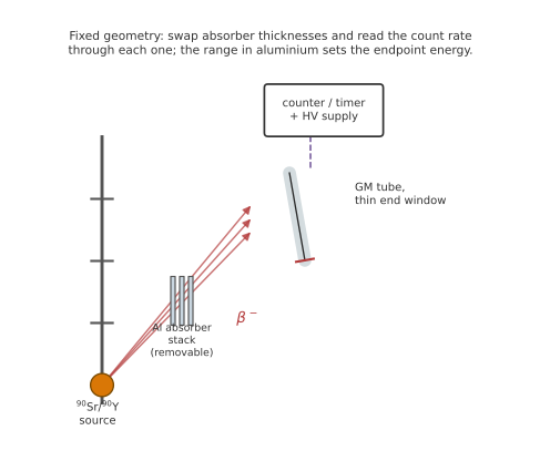
A sealed beta source sits on the lowest shelf of a stand, emitting electrons through an interchangeable aluminum absorber stack toward a Geiger–Müller tube connected to a counter and timer. — Figure 3.2:The fixed source-absorber-tube geometry. Swapping absorber thicknesses and reading the transmitted count rate through each maps the range of the beta electrons in aluminum.

Procedure¶

Before you count¶

Match the source, absorber shelf, and GM-tube order to Figure 3.2. Record the shelf number and source-to-window distance; the sketch does not specify those dimensions for your apparatus.
Inspect the thin detector window without touching it. Confirm that the source holder, absorber tray, and detector cannot shift when foils are exchanged.
List every absorber in increasing areal density and record its labeled value before starting. Keep the foils in that order so that a thickness is never inferred from appearance.
Prepare separate tables for the plateau, background, and absorption scan. Every counting row must contain raw counts, live time, high voltage, absorber identity, and geometry notes—not only a displayed count rate.
Estimate counting times in advance: choose them so useful absorption points have roughly similar fractional Poisson uncertainty. Ask the instructor to handle or relocate any source not explicitly assigned to students.

Part A — The plateau and the operating voltage¶

Use the instructor-approved voltage range and source shelf. If students are authorized to measure the plateau, follow the tube’s procedure for voltage steps and count duration, and plot rate against voltage as you go. Otherwise, record the approved operating voltage and skip the scan.
Identify a stable plateau if a scan is performed. Use the operating voltage approved for this specific tube; do not infer a universal offset above the knee.

[ ] Checkpoint 1. Show the instructor your plateau plot or the approved operating setting before taking source data. Do not increase voltage beyond the specified operating range.

Part B — Background¶

Return the source to its shielded storage. Count the background for at least $10\ \text{minutes}$ in a single run and record $N_{\text{bg}}$ and the live time. Use this rate to calculate net source rates; the terminal range fit below uses gross rates so the shared background estimate does not introduce correlations.
Note the counts, not just the rate; you need $N$ to get the Poisson uncertainty.

Part C — The absorption curve¶

Place the source on the assigned fixed shelf and do not move it again — a changed source–detector geometry changes detection efficiency and can masquerade as absorption. The near-field geometry does not generally obey a simple inverse-square law.
Count with no absorber. Aim for about $10\,000$ counts if the detector is within its validated count-rate range; otherwise follow the instructor’s lower-rate geometry or timing plan.
Add absorbers in increasing mass thickness. Use roughly 10–15 values, placing more points near the predicted $^{90}$ Y endpoint than in the rapidly falling low-thickness region. Record the total stack thickness for every setting.
Increase counting time as the rate falls, especially in the terminal region. Estimate the time budget before beginning: at $2\ \text{s}^{-1}$ , 100 counts take 50 s but a 1% Poisson measurement takes 5,000 s. The latter is not a reasonable target for every point in a three-hour period.
If the absorber set extends beyond the terminal fall, take at least four thick-absorber points to characterize the floor. If the measured rate is still falling at the thickest available setting, record the limitation; do not extrapolate an unobserved floor into a claimed endpoint.
Verify two or three of the absorbers’ labeled mass thicknesses by weighing them and measuring their area. Foil labels are sometimes optimistic.

Analysis¶

Rates and their uncertainties¶

For each point, the net rate and its uncertainty, before any dead-time correction, are

R = \frac{N}{t} - \frac{N_{\text{bg}}}{t_{\text{bg}}}, \qquad \sigma_R = \sqrt{\frac{N}{t^2} + \frac{N_{\text{bg}}}{t_{\text{bg}}^2}} .

(3.7)

The same background estimate appears in every net rate, so those net values are correlated. Plot them to see the source contribution, but fit the independent gross rates $N/t$ in the terminal and floor regions below. A negative net rate is possible after background subtraction and is not a negative physical activity.

Check dead-time losses at the largest gross rate using the instrument’s measured or specified dead time. For a nonparalyzable model, the correction is $R_{\text{true}}=R_{\text{obs}}/(1-R_{\text{obs}}\tau_d)$ when $R_{\text{obs}}\tau_d<1$ . It is not a universal GM-tube law or a substitute for operating below the instrument’s rated count rate. Near the endpoint, where the rate is low, dead time should have little effect; document that check. See the IAEA detector-model discussion.

Finding the range¶

First plot gross count rate against aluminum mass thickness on both log and linear rate axes. The log view shows the full fall; the linear view reveals the terminal region and the measured floor. Select a contiguous terminal region dominated by the $^{90}$ Y component, after the low-energy $^{90}$ Sr component has largely disappeared, and a separate set of thick-absorber points whose rates are consistent with a constant floor. Do not fit the steep initial semilog line and call its intersection with an arbitrary noise threshold a physical range.

Fit a straight line to the terminal gross rates and take its intersection with the independently measured floor. In the example below, choose the three thickness boundaries from your plot; keep the terminal and floor selections disjoint.

import numpy as np
from scipy.optimize import curve_fit

x = np.array([...], dtype=float)       # aluminum mg/cm^2, one value per run
N = np.array([...], dtype=float)       # gross counts
t = np.array([...], dtype=float)       # live time in seconds

x_fit_start, x_fit_end, x_floor_start = ... , ... , ...
terminal = (x >= x_fit_start) & (x <= x_fit_end)
tail = x >= x_floor_start
assert terminal.sum() >= 3 and tail.sum() >= 4
assert not np.any(terminal & tail)
assert np.all(N[terminal | tail] > 0)   # use a Poisson fit for zero-count bins

rate = N / t
srate = np.sqrt(N) / t
w = 1 / srate[tail]**2
floor = np.sum(w * rate[tail]) / np.sum(w)
sfloor = np.sqrt(1 / np.sum(w))

def terminal_line(x, a, b):
    return a + b * x

(a, b), cov = curve_fit(terminal_line, x[terminal], rate[terminal],
                        sigma=srate[terminal], absolute_sigma=True)
assert b < 0
Rm = (floor - a) / b             # aluminum thickness, mg/cm^2
g = np.array([-1 / b, -(floor - a) / b**2])
sRm = np.sqrt(g @ cov @ g + (sfloor / b)**2)
print(f"practical range = {Rm:.0f} +/- {sRm:.0f} mg/cm^2")

The covariance term in sRm matters because fitted slope and intercept are correlated. This statistical error is only one part of the range uncertainty. Vary the terminal fit window and the choice of floor points, inspect the residuals, and include the resulting model sensitivity. If the floor is not observed or the terminal segment is not approximately linear, report a lower bound or an unresolved endpoint instead of a precise energy.

Energy and speed¶

Invert both range–energy relations:

from scipy.optimize import brentq

Rm_g = Rm / 1000.0                                   # g/cm^2

T_feather = (Rm_g + 0.133) / 0.542                   # MeV

def kp(T):                                            # Katz-Penfold, implicit
    n = 1.265 - 0.0954 * np.log(T)
    return 412 * T**n - Rm                            # Rm in mg/cm^2

T_kp = brentq(kp, 0.8, 2.5)             # stay within the energy range used here

mec2  = 0.51099895                                    # MeV
gamma = 1 + T_kp / mec2
beta  = np.sqrt(1 - 1/gamma**2)
pc    = np.sqrt((T_kp + mec2)**2 - mec2**2)
beta_classical = np.sqrt(2 * T_kp / mec2)

Report $T_{\max}$ from both relations and propagate the uncertainty in $R_m$ by recomputing each energy at $R_m \pm \sigma_{R_m}$ . Their difference is a useful model comparison, but it is not a complete estimate of calibration or fit-window uncertainty. If the numerical root is not bracketed in the stated energy range, do not extrapolate this calibration without justification. If the range was only bounded, invert that bound and report the energy as a bound too.

Post-lab questions¶

Going further¶

Several sources, one calibration. If approved sources with distinct known beta endpoints are available, measure a practical range for each with a common geometry and fit an empirical range–energy relation. A mixed $^{90}$ Sr/ $^{90}$ Y source does not automatically give two separately measurable practical ranges. Compare your calibration with Katz–Penfold.
Absorber material dependence. Repeat a few points using plastic or copper absorbers of the same mass thickness. Compare their curves without assuming equal stopping power per unit mass, especially for copper. A changed thick-absorber floor may reflect photon production or detector response; it does not by itself measure a simple $Z^2$ law.
The Kurie plot. With a scintillator and a multichannel analyzer instead of a GM tube, an energy spectrum can be recorded and analyzed with a Kurie plot, subject to detector resolution and calibration. Precision neutrino-mass experiments require much finer control of the spectrum near an endpoint than this teaching apparatus provides.