Experiment 11 — Alkali Spectra, Screening, and the Quantum Defect¶
Objectives¶
By the end of this experiment you should be able to:
Test whether the spectrometer resolves the sodium D doublet, measure its splitting if it does, and interpret it as spin–orbit coupling.
Assign observed sodium lines to transitions and, where the faint lines are detected, infer state-specific quantum defects from their level energies and an independent ionization limit.
Explain why the quantum defect decreases sharply with increasing , in terms of the penetration of the valence orbital into the core.
Explain why hydrogen’s simple-Coulomb degeneracy is generally broken in many-electron atoms.
Textbook connection¶
Read §11.1–11.6. Chapter 10 established that hydrogen’s energies depend only on . Chapter 11 explains why every other atom is different: the valence electron of an alkali sees a nuclear charge that is screened by the closed inner shells, and the degree of screening depends on how much the orbital penetrates the core — which depends on . The optional weak-line measurements probe that dependence.
The X-ray apparatus this laboratory once used for Moseley’s law is no longer serviceable. Quantum defects and Moseley’s law both involve electron screening, but they probe different orbitals and different energy scales.
Theory¶
The quantum defect¶
For a single valence electron outside a closed-shell core, an energy level measured relative to the ionization limit is often described by a Rydberg formula with a shifted principal quantum number:
where is the quantum defect, identifies a resolved fine-structure level, and includes the sodium ion’s reduced mass. A defect changes slowly with within a series but is not strictly constant, especially for low- states. For sodium, representative values for the lowest available states are
These values use the NIST sodium levels and ionization limit and its extended Na I level compilation with a leading-order Rydberg model. The defect is about 1.353, so carrying unchanged to another can matter. The D-line prediction is sensitive to the rounded and defects; compare it at the precision the model and wavelength convention support.
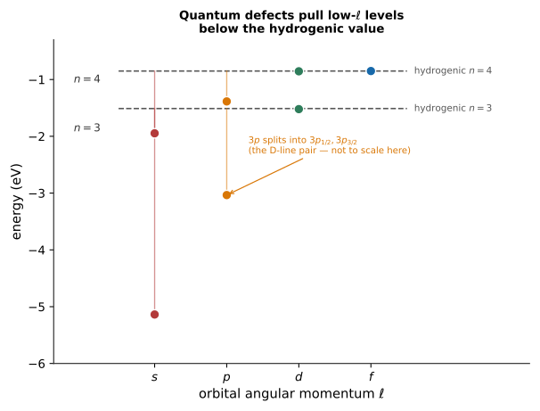
Figure 11.1:Quantum defects for allowed states at and . The dashed lines show a hydrogenic reference for each ; penetration into the core pulls and levels down most. The orbital labels obey .
The physical reading: a low- orbital has appreciable probability density near the nucleus, where it sees the unscreened nuclear charge rather than the long-range ionic-core charge near +1. It is therefore bound more tightly than a hydrogenic level of the same , and measures the extra binding in units of a principal quantum number. High- orbitals are kept out of the core by the centrifugal barrier , see a long-range Coulomb charge near +1, and are almost hydrogenic — which is why and defects are much smaller than defects.
The series¶
Transitions in an alkali obey , and the classical spectroscopic series are
Sodium series (all terminating on or starting from low-lying states)
Series | Transition | Accessible member or note |
|---|---|---|
Principal | Strongest in absorption; includes the D lines at | |
Sharp | Includes the visible pair near 615 nm | |
Diffuse | Includes the visible group near 568 nm | |
Fundamental | In the infrared |
The letters , , , — now the standard orbital labels throughout physics and chemistry — are the initials of sharp, principal, diffuse, and fundamental: the names of these spectral series, assigned before anyone knew what an orbital was.
Spin–orbit splitting¶
The D “line” of sodium is two standard-air lines, at 588.995 and — a separation of , or about . The level is split by the spin–orbit interaction into and ; the ground state has no spin–orbit doublet. Potassium’s principal doublet is near , outside the range of some visual spectrometers and detectors. Its different splitting reflects both nuclear charge and the valence electron’s orbital penetration; no universal rule predicts it from sodium alone.
Measuring this splitting tests the relativistic spin–orbit interaction in an atomic spectrum. The simple magnetic-field picture is only an approximation for an alkali electron moving through a screened core potential.
Pre-lab¶
Apparatus¶
Sodium discharge lamp or sodium spectral tube, with the warm-up time specified for that source; some sodium lamps show startup-gas lines before stabilizing
Mercury and helium lamps for calibration
Calibrated grating spectrometer or EDU-SPEB2 kit. Test the actual resolution with nearby reference lines; a narrow slit helps only until signal and the instrument profile limit the result. Weak-line detection depends on source brightness, detector sensitivity, and spectral coverage.
Neutral-density filters for a detector that would saturate on the D lines at the settings needed for weaker members
Optionally: potassium or lithium lamps for a qualitative doublet comparison
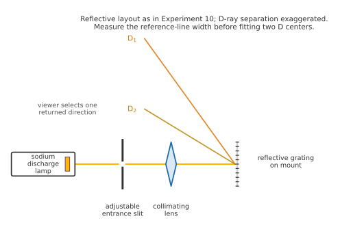
Figure 11.2:The reflective-grating layout from Experiment 10, now with sodium. The D-ray separation is exaggerated; resolve the pair experimentally before reporting two centers.
Procedure¶
Before you search for weak lines¶
Use Figure 11.2 to identify the same calibrated spectrometer geometry used in Experiment 10. The labeled D rays show why resolution is needed; their separation in the drawing is deliberately exaggerated.
Warm the alkali lamp until its intensity is stable. Keep the lamp supply covered, switch it off before exchanging lamps, and avoid touching a hot envelope.
Record grating, slit width, spectral order, and viewing or detector method. For a detector, record integration time and gain and save a dark spectrum for each setting used for faint lines.
Prepare a search list from the NIST reference data, with predicted wavelength, transition, observed wavelength, trial count, signal-to-noise ratio, and assignment confidence. Also keep an “unassigned” list.
Take an overview spectrum before narrowing the slit. Use that spectrum to navigate, but use unsaturated high-resolution scans for line centers; do not extract the D splitting from a clipped overview.
Part A — Calibration, again¶
Calibrate the actual grating geometry or pixel scale as in The Balmer Series and the Rydberg Constant, using resolved mercury lines and, if needed to cover 615 nm, the helium line near 667.8 nm as a calibration anchor or held-out check. State which role each line has. Resolve the mercury yellow lines at 576.96 and as a preliminary instrument check.
Record calibration residuals and a held-out check. Measure the width of an isolated narrow reference line near the D region at the same slit and detector settings. A width well below and adequate sampling are needed to attempt the D splitting; resolving the 2.1 nm mercury pair alone does not demonstrate this.
[ ] Checkpoint 1. Show the calibration and measured reference-line width. Decide whether the instrument can plausibly separate the D lines, and record the limitation if it cannot.
Part B — The D doublet¶
Let the sodium lamp warm up fully. Attenuate it.
Locate the D feature. Narrow the slit while tracking signal and line width; fit or read two centers only if the pair is resolved under those settings.
If resolved, measure both wavelengths at least five times each. Alternate approach direction on a vernier instrument to expose backlash. If not resolved, record one feature and a resolution limit instead.
Record the slit width and, if possible, repeat at two slit widths to check for a slit-dependent shift.
[ ] Checkpoint 2. Show the instructor the D profile, your measured splitting or resolution limit, and the settings used.
Part C — The series¶
Remove attenuation, adjust exposure without saturating, and search for the group near 568 nm and pair near 615 nm. These are much fainter than the D lines; measure background at each detector setting.
Measure as many independent centers as the instrument can resolve. In particular, the two components near 568.819 and 568.821 nm will normally form one blend. Report non-detections with the achieved sensitivity rather than inventing six extra lines.
Assign each to a transition using your table, and record which assignments you are confident in and which you are not. An honest “unassigned” is better than a forced assignment. Recheck a blue and red calibration line at the settings used for the weak lines and include any drift.
Part D (optional) — Another alkali¶
If a potassium lamp and suitable near-IR detector are available, test its principal doublet near 766.5/769.9 nm. If using lithium near 671 nm, check whether the instrument can actually resolve its much closer pair before reporting a splitting.
Analysis¶
The splitting¶
If both D centers are resolved, report their separation and convert to using vacuum wavelengths, with the shorter:
This is a small difference of two nearby numbers. Propagate the covariance of the calibrated line centers: a common wavelength offset can largely cancel in the splitting, while uncertainty in the dispersion scale does not. See Uncertainty and Curve Fitting. If unresolved, report the observed width and the inability to determine the splitting under those settings. An upper limit requires a justified instrument-profile model.
Quantum defects¶
Use measured vacuum wavenumbers to reconstruct levels above the ground state. D is and D is . The visible sharp-series line near 615.4225 nm is ; the unblended diffuse-series line near 568.2633 nm is . These assignments and approximate standard-air wavelengths come from the NIST Na I line data and level compilation. Thus, in inverse metres,
With the independent NIST Na I ionization limit , derive a defect for each measured state from
Here accounts approximately for the reduced mass of the sodium ion. A term-average level can be formed as ; the weights are the fine-structure degeneracies . Keep the -resolved levels when comparing individual observed lines.
The following code assumes all four indicated centers were measured. Supply their vacuum wavelengths in the specified order and the full wavelength covariance matrix, including shared calibration terms:
import numpy as np

R_Na = 1.097347e7          # m^-1, approximate sodium reduced-mass value
T_limit = 41449.451 * 100  # m^-1, external NIST reference
lam = np.array([...])       # vacuum meters: D1, D2, 615.4225, 568.2633
C_lam = np.array([...])     # 4 x 4 covariance of these wavelengths, m^2

def defects(wavelengths):
    nu = 1.0 / wavelengths
    T_p = (nu[..., 0] + 2 * nu[..., 1]) / 3  # 3p term average
    T_s = nu[..., 0] + nu[..., 2]           # 5s from D1 and 615.4
    T_d = nu[..., 0] + nu[..., 3]           # 4d_3/2 from D1 and 568.3
    T = np.stack([T_p, T_s, T_d], axis=-1)
    return np.array([3, 5, 4]) - np.sqrt(R_Na / (T_limit - T))

delta = defects(lam)        # 3p average, 5s, 4d_3/2
rng = np.random.default_rng(11)
draws = rng.multivariate_normal(lam, C_lam, size=10000)
s_delta = defects(draws).std(axis=0, ddof=1)
for name, value, uncertainty in zip(("3p", "5s", "4d_3/2"), delta, s_delta):
    print(f"delta_{name} = {value:.4f} +/- {uncertainty:.4f}")
Use the line-center covariance from calibration and repeats when estimating these uncertainties. Vary the air-index conversion and ionization limit if their uncertainties matter at your precision. The measured D pair and external limit can give a defect; and defects require their respective weak lines. The defect computed from the external limit alone is a reference value, not a quantity measured by this experiment. Compare with that reference, noting that an -independent defect is only an approximation.
Screening¶
For each measured state, calculate an energy-equivalent effective charge: the charge that would give the same binding energy in a hydrogenic formula at the same :
Report only for states whose defects you determined. This single number summarizes binding energy; the physical screening varies with radius and is not a measured constant charge. Compare the values with the long-range ionic-core charge +1 and bare nuclear charge +11.
Post-lab questions¶
Going further¶
The Zeeman effect. With an approved magnet and optical geometry, the sodium D profiles can show additional polarization-dependent components. Predict the allowed transitions and compare their separation with your measured instrumental width before attempting to resolve them.
Absorption instead of emission. With an approved heated sodium vapor cell and broadband source, the D lines can appear in absorption, as they do among the solar Fraunhofer lines.
Rydberg states. With wider spectral coverage and adequate sensitivity, follow several members of one series toward its limit. Fit their level energies to determine the ionization limit and examine how its quantum defect changes with ; a visible-only scan of the D and weak pairs does not establish the series limit.