Learning Objectives
By the end of this chapter, you should be able to:
Distinguish ionic and covalent bonding in terms of the underlying electron distribution.
Explain covalent bond formation in valence bond theory as the overlap of atomic orbitals.
Explain the need for hybrid orbitals and identify the hybridization and molecular geometry implied by a given number of electron domains.
Construct molecular orbitals as linear combinations of atomic orbitals and distinguish bonding from antibonding orbitals.
Use a molecular orbital diagram to compute bond order and predict the stability and magnetic behavior of a simple diatomic molecule.
Explain the vibrational and rotational energy levels of a diatomic molecule using the harmonic-oscillator and rigid-rotor approximations.
Introduction
Chapters 10 and 11 explained the structure of individual atoms — how electrons occupy discrete energy levels arranged into subshells and shells, and how that arrangement produces the periodic table. This chapter asks how atoms combine to form molecules, using the same quantum-mechanical toolkit: atomic orbitals, the Pauli exclusion principle, and the variational tendency of a bound system to seek its lowest-energy configuration. Two complementary pictures are developed. Valence bond theory treats a bond as the overlap of atomic orbitals from two atoms, localized between them, and is the natural language for molecular geometry. Molecular orbital theory instead builds orbitals belonging to the molecule as a whole, and is the more powerful tool for predicting a molecule’s stability, bond strength, and magnetic properties. The chapter closes by treating a bonded diatomic molecule as a single quantum system in its own right, subject to quantized vibrational and rotational energy levels — a direct application of the harmonic oscillator (Chapter 8) and angular momentum quantization (Chapter 9) to a new physical system.
12.1Bonding and Hybrid Orbitals
Ionic and Covalent Bonding
Chemical bonds form because a molecule can have lower total energy than its constituent separated atoms. Two limiting mechanisms produce this energy lowering. In ionic bonding, one atom (typically one with a low ionization energy, such as an alkali metal) transfers one or more electrons entirely to another atom (typically one with a high electron affinity, such as a halogen); the resulting oppositely charged ions are then held together by simple electrostatic (Coulomb) attraction. In covalent bonding, by contrast, one or more electron pairs are shared between two atoms, occupying a region of enhanced electron density between the two nuclei; both nuclei are then simultaneously attracted to this shared, concentrated negative charge, producing a net attractive bond. Most real bonds fall on a continuum between these two limits, described by varying degrees of bond polarity, depending on the difference in electronegativity between the bonded atoms; this chapter focuses on the covalent limit, whose treatment requires genuinely quantum-mechanical ideas beyond simple electrostatics.
That continuum is a slider rather than a classification, and Figure 12.1 makes it one: set the electronegativity of each atom in a diatomic and watch the shared electron density slide from the midpoint toward the more electronegative partner, dragging a dipole moment with it. At equal electronegativity the bond is purely covalent and the dipole vanishes; at a large difference the electron is effectively transferred and what remains is a pair of ions attracting each other. Neither limit is a separate mechanism — they are the two ends of one.
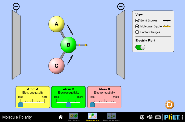
Figure 12.1:Bond polarity as a continuous function of the electronegativity difference between two atoms, with the electron density and the resulting dipole moment displayed. Later screens add a third atom, where bond dipoles combine vectorially and a molecule of polar bonds can still be nonpolar overall.
Interactive simulation: Molecule Polarity
Valence Bond Theory and Orbital Overlap
Valence bond theory treats covalent bond formation as arising from the overlap of a singly occupied atomic orbital on one atom with a singly occupied atomic orbital on another, the two electrons (one from each atom, necessarily of opposite spin, per the exclusion principle applied to the resulting shared, doubly occupied region) pairing up to form the bond. The simplest example is the hydrogen molecule : as two hydrogen atoms approach, their orbitals begin to overlap, and if the two electrons involved have opposite spin, the resulting overlap region between the nuclei has a high joint probability of finding both electrons — an enhanced electron density that lowers the system’s total energy relative to two separate atoms, up to a certain optimal internuclear separation (the bond length, at which attractive and repulsive contributions to the energy balance). Bonds formed by orbitals overlapping directly along the internuclear axis, giving a cylindrically symmetric electron distribution about that axis, are called sigma () bonds; bonds formed by the sideways overlap of parallel orbitals, with electron density concentrated above and below (rather than directly along) the internuclear axis, are called pi () bonds. A single bond is one bond; a double bond is one plus one bond; a triple bond is one plus two (mutually perpendicular) bonds.
Hybrid Orbitals
Simple atomic and orbitals, taken directly from the hydrogen-like solutions of Chapter 10, generally point in the wrong directions (or have the wrong shapes) to account for the observed bond angles and geometries of real molecules — the observed near- bond angles of methane, , for instance, are not reproduced by combinations of the atom’s unmodified and three orbitals directly. The resolution is that the atomic orbitals actually used in bonding are not the pure , , orbitals of an isolated atom, but specific linear combinations of them, called hybrid orbitals, that better match the geometry demanded by minimizing electron-pair repulsion among the atom’s bonding and lone electron pairs (the same qualitative principle underlying the electron-domain, or VSEPR, geometries encountered in general chemistry). Mixing one orbital with a varying number of (and, for some geometries, ) orbitals produces hybrid sets with characteristic, experimentally matched geometries:
The standard geometries are collected in Table 12.1.
Table 12.1:Common orbital hybridizations and their molecular geometries
| Hybridization | Orbitals mixed | Number of hybrids | Geometry | Example |
|---|---|---|---|---|
| one , one | 2 | linear () | ||
| one , two | 3 | trigonal planar () | ||
| one , three | 4 | tetrahedral () | ||
| one , three , one | 5 | trigonal bipyramidal | ||
| one , three , two | 6 | octahedral |
For the five- and six-domain cases, and are traditional hybridization labels that summarize the electron-domain geometry. They should not be read as evidence that occupied valence orbitals are literally needed to form the bonds in hypervalent molecules such as and ; modern bonding descriptions account for these molecules without substantial -orbital participation.
The general rule connecting geometry to hybridization is that the number of hybrid orbitals equals the number of electron domains around the central atom — bonding pairs plus lone pairs — and that hybrid orbitals arrange themselves to maximize their mutual angular separation, minimizing electron-pair repulsion, exactly as in the VSEPR (valence-shell electron-pair repulsion) model of molecular geometry. Unshared (lone) electron pairs occupy hybrid orbitals just as bonding pairs do, but exert somewhat greater repulsion (being attracted to only one nucleus rather than shared between two), which is why, for example, the bond angle in water (, two bonding pairs and two lone pairs on an approximately oxygen) is compressed to about from the ideal tetrahedral .
The counting rule behind Table 12.1 is worth exercising on molecules other than the five listed, and Figure 12.2 is set up for exactly that: attach single, double, or triple bonds and lone pairs to a central atom in any combination and the geometry rearranges itself, with the bond angles reported as they change. Two predictions from the paragraph above can be checked in a few seconds there. A double bond and a single bond count the same for geometry — both are one electron domain — and replacing a bonding pair by a lone pair squeezes the remaining angles, reproducing water’s from tetrahedral.
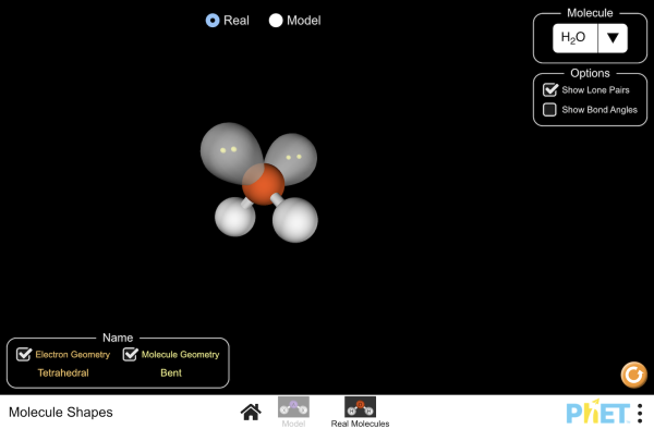
Figure 12.2:Molecular geometry built from electron domains. Bond angles are displayed live, and the “real molecules” screen compares the idealized VSEPR prediction with measured geometries.
Interactive simulation: Molecule Shapes
Worked Example: The Geometry of Xenon Tetrafluoride
Predict the hybridization and molecular geometry of .
Xenon forms four Xe–F bonds to the four fluorine atoms. After those four bonding pairs and the three lone pairs required on each fluorine to complete its own octet are accounted for, the count of xenon’s eight valence electrons leaves two lone pairs on xenon itself — xenon, unlike carbon or nitrogen, has enough valence electrons to bond fully and retain lone pairs of its own. The central atom therefore has 4 bonding domains lone pairs electron domains, calling for hybridization and an octahedral arrangement of those six domains.
The two lone pairs could sit at (adjacent) or (opposite) to each other on the octahedron. Because lone-pair–lone-pair repulsion is the strongest of the three repulsion types recognized by the electron-domain model (lone pair–lone pair lone pair–bonding pair bonding pair–bonding pair), the two lone pairs move as far apart as the octahedral geometry allows: directly opposite one another. That leaves the four Xe–F bonds occupying the remaining four positions, all in a single plane — a square planar molecular geometry, with –– bond angles of exactly between adjacent fluorines and across. This result is worth remembering precisely because the naive guess for “four bonded groups” — tetrahedral, as in — is wrong here: the two lone pairs, invisible in a skeletal formula, are what flatten the molecule into a plane.
12.2Molecular Orbital Theory
Valence bond theory, with hybridization added, accounts well for molecular geometry, but it treats bonding electrons as localized between two specific atoms and struggles to describe phenomena in which electrons are shared more broadly, or where a simple bonding picture predicts the wrong number of unpaired electrons. Molecular orbital (MO) theory instead constructs orbitals belonging to the molecule as a whole, built as linear combinations of the atomic orbitals (LCAO) of the constituent atoms, exactly as a molecular wave function must ultimately be some solution of the (approximate, many-electron) Schrödinger equation for the whole molecule.
For two hydrogen orbitals, and , on atoms and , the two independent linear combinations are
The symmetric combination, , adds constructively in the region between the two nuclei, producing enhanced electron density there and a lower energy than the separate atomic orbitals — a bonding orbital, denoted . The antisymmetric combination, , has a node exactly at the midpoint between the nuclei, depleting electron density in the internuclear region and yielding a higher energy than the separate atomic orbitals — an antibonding orbital, denoted . In general, combining atomic orbitals produces exactly molecular orbitals (never more, never fewer) — a direct consequence of treating the LCAO expansion as a change of basis for the same underlying space of trial wave functions. The resulting orbitals can be bonding, antibonding, or, when an orbital has little net interaction with the others, nonbonding; the bonding and antibonding energies need not be symmetrically displaced from the original atomic-orbital energy.
Why the Antibonding Orbital Rises More Than the Bonding Orbital Falls
The qualitative claim that is lower in energy and is higher can be made quantitative. Define three integrals: the overlap integral (how much the two atomic orbitals overlap in space, ), the Coulomb integral (essentially the original atomic-orbital energy, perturbed by the presence of the other nucleus), and the resonance integral (negative, and nonzero only because the orbitals overlap). Normalizing and evaluating gives
Because , and because is large enough compared to for essentially every real covalent bond (the case of interest here), lies below (bonding) and lies above (antibonding) — but the two shifts are not equal in magnitude. The in the antibonding denominator is smaller than the in the bonding denominator, so rises above by more than falls below it. This asymmetry is the entire reason fails to bond: two electrons in and two in do not cancel to zero net energy change, because the antibonding pair’s destabilization outweighs the bonding pair’s stabilization, leaving at higher energy than two separate helium atoms — consistent with, and quantitatively explaining, the bond order of zero found by simple electron counting below.
Filling the resulting molecular orbitals with the molecule’s electrons, two at a time (spin-paired, per the exclusion principle applied now to molecular rather than atomic orbitals) from lowest to highest energy, gives a molecular orbital diagram, from which the bond order is computed as
A bond order of zero predicts no net covalent energy lowering relative to separated atoms; a bond order of corresponds roughly to a single, double, triple, bond, with higher bond order generally correlating with a shorter, stronger bond. For (two electrons, both in ), the bond order is , consistent with the known stable single bond; for the hypothetical (four electrons, two in and two forced by the exclusion principle into ), the bond order is — correctly predicting that has no conventional covalent bond, a conclusion valence bond theory (which has no natural way to place electrons in an antibonding orbital) does not straightforwardly reach. A neutral helium dimer can nevertheless exist as an extraordinarily weak van der Waals-bound state, an intermolecular effect outside this simple covalent MO diagram. MO theory additionally predicts a molecule’s magnetic behavior directly from its orbital diagram: any unpaired electrons (occurring, per Hund’s rule applied to degenerate molecular orbitals, when a set of same-energy orbitals is only partially filled) make the molecule paramagnetic (weakly attracted into a magnetic field), while a fully paired configuration makes it diamagnetic (weakly repelled) — famously correctly predicting that is paramagnetic (two unpaired electrons in degenerate antibonding orbitals), a fact simple Lewis-structure/valence-bond reasoning does not anticipate.
The bonding and antibonding pair are not a chemical convention; they are what the Schrödinger equation returns for two wells brought close together, and Figure 12.3 solves that problem directly. Start with two widely separated square wells: each has its own ground state, and the two are degenerate. Slide them together and the degeneracy lifts into exactly two states — one symmetric, with no node between the wells and an energy below the isolated-atom level, and one antisymmetric, with a node at the midpoint and an energy above it. That is and , obtained without mentioning chemistry, and the splitting between them grows as the wells approach, which is why bond strength depends on overlap.
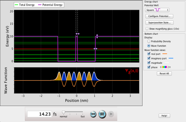
Figure 12.3:A double square well with adjustable separation and depth, and the eigenstates it supports. The symmetric–antisymmetric splitting of a pair of formerly degenerate levels is the origin of the bonding/antibonding pair of MO theory, and — extended to wells in a row — of the energy bands of a solid.
Interactive simulation: Double Wells and Covalent Bonds
Historical Context: From Lewis’s Electron Pair to the Pauling–Mulliken Rivalry
The idea that a covalent bond is a shared pair of electrons predates quantum mechanics itself. In 1916 — a full decade before Schrödinger’s equation — the American chemist Gilbert N. Lewis proposed exactly this picture, together with the electron-dot notation still used to sketch molecules today, purely from chemical reasoning about valence and the stability of the noble-gas electron count, with no wave mechanics available to justify it. Lewis’s shared pair was a hypothesis in search of a mechanism, and quantum mechanics supplied one a decade later, in two competing forms.
Valence bond theory, developed by Walter Heitler and Fritz London (1927) and then extended and popularized by Linus Pauling through the early 1930s — including the hybrid-orbital concept of this chapter — kept Lewis’s picture of a bond as a localized pair shared between two specific atoms, now computed from overlapping atomic wave functions rather than guessed at. Molecular orbital theory, developed in the same years chiefly by Friedrich Hund and Robert Mulliken, instead discarded the idea that an electron belongs to one bond at a time, building orbitals delocalized over the whole molecule from the outset. The two camps disagreed, sometimes sharply, over which picture was the physically correct starting point — Pauling’s localized, chemist-friendly bonds versus Mulliken’s delocalized, spectroscopically motivated orbitals — and valence bond theory, propelled by Pauling’s enormously influential 1939 book The Nature of the Chemical Bond, remained the dominant teaching framework through the 1950s. Molecular orbital theory eventually overtook it, in no small part on the strength of results like the paramagnetism prediction below, which valence bond theory cannot produce without ad hoc patching. Pauling received the 1954 Nobel Prize in Chemistry “for his research into the nature of the chemical bond,” and Mulliken received the 1966 Prize “for his fundamental work concerning chemical bonds and the electronic structure of molecules by the molecular orbital method” (Figure 12.4). Both theories remain in active use today, each suited to different questions — geometry and localized reactivity for valence bond theory, spectra and magnetism for molecular orbital theory — which is why this chapter, like the field itself, teaches both.
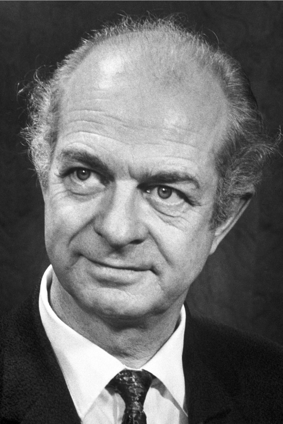
Figure 12.4:Linus Pauling, photographed in 1962, eight years after his 1954 Nobel Prize in Chemistry for work on the nature of the chemical bond — the valence-bond and hybridization framework of this chapter. Photograph by the Nobel Foundation; public domain via Wikimedia Commons.
Building the Diagram for the Second Row: N₂ and O₂
Hydrogen and helium have only orbitals to combine, but a second-row diatomic such as or has both and atomic orbitals on each atom, and the resulting molecular orbital diagram, while built by exactly the same LCAO recipe used for , has more structure worth spelling out explicitly.
Combining the two orbitals (one per atom) gives a bonding and an antibonding , exactly as for . Of the three orbitals on each atom, the pair pointing directly along the internuclear axis overlaps head-on, giving a bonding and antibonding ; the two remaining pairs of orbitals, oriented perpendicular to the axis, overlap sideways, giving a bonding and antibonding pair for each of the two independent perpendicular directions — so the level (and, separately, the level) is doubly degenerate, two orbitals at the same energy. In all, eight atomic orbitals (one and three on each of two atoms) combine into eight molecular orbitals: , , , , and the degenerate pairs and .
The one genuine subtlety is the relative energy of and , and it is worth getting right because it is a famous trap. Head-on () overlap is intrinsically stronger than sideways () overlap, so a naive picture would put below always — and that is indeed the order for , , and . But for the lighter diatomics , , and , the order inverts: sits below . The mechanism is – mixing: and share the same symmetry along the internuclear axis, and whenever the atomic and energies are close enough, these two molecular orbitals mix with each other quantum mechanically, pushing lower and higher than a naive non-interacting picture would predict — enough, for the lighter elements, to push above entirely. Moving across the period, increasing nuclear charge pulls the orbital down in energy faster than the orbital (a electron spends more time near the nucleus and so feels the increasing charge more strongly), widening the – gap; by oxygen, that gap is wide enough that – mixing is too weak to invert the order, and the naive -below- sequence is restored. Figure 12.5 shows both diagrams side by side, filled with electrons.
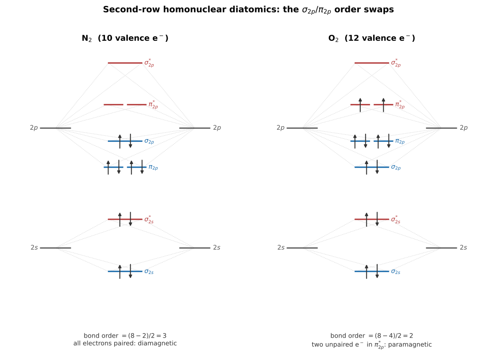
Figure 12.5:Molecular orbital diagrams for N and O. Atomic and levels sit outside; molecular orbitals sit in the middle, filled from the bottom with the molecule’s valence electrons. Note the swapped order: below for N (light diatomic, strong – mixing), below for O (heavier, weak – mixing). Original schematic generated with matplotlib; see scripts/figures/.
For (10 valence electrons), filling from the bottom — (2), (2), (4), (2) — uses all ten electrons with every orbital either completely filled or completely empty, giving
consistent with the triple bond of the Lewis structure , and, with every electron paired, correctly predicting that is diamagnetic.
Worked Example: The Molecular Orbital Diagram and Paramagnetism of O₂
Construct the molecular orbital diagram for , determine its bond order, and explain its paramagnetism.
has valence electrons. Using the heavier-diatomic ordering established above — , , , (), (), — fill from the bottom, two electrons per orbital, respecting Hund’s rule (spread electrons across a set of degenerate orbitals, one each, before pairing any of them), as in Table 12.2:
Table 12.2:Filling the O2 molecular orbital diagram
| Orbital | Electrons added | Running total |
|---|---|---|
| 2 | 2 | |
| 2 | 4 | |
| 2 | 6 | |
| (both orbitals) | 4 | 10 |
| (both orbitals) | 2 | 12 |
The last two electrons enter the doubly degenerate level. Hund’s rule places one electron in each of the two degenerate orbitals, with parallel spins, rather than pairing both into a single orbital — leaving two unpaired electrons. Counting bonding electrons (: 2, : 2, : 4, total 8) against antibonding electrons (: 2, : 2, total 4),
consistent with the double bond of the Lewis structure . But that Lewis structure, with every electron paired off into bonds and lone pairs, gives no hint of the two unpaired electrons found here — and it is exactly those two unpaired electrons that make liquid oxygen paramagnetic, visibly drawn toward the poles of a strong magnet in the standard classroom demonstration, a fact valence bond theory cannot explain without modification but that falls directly out of the molecular orbital diagram.
Bond Order, Bond Length, and Bond Strength: A Worked Comparison
Bond order is a prediction about two directly measurable quantities: bond length and bond dissociation energy. Higher bond order means more shared electron density concentrated between the nuclei, which pulls the nuclei closer together (shorter bond length) and requires more energy to pull them apart (higher dissociation energy). The nitrogen–nitrogen bond, compared across three different molecules in Table 12.3, shows the trend cleanly, because in each case the bond order is unambiguous from the Lewis structure:
Table 12.3:Nitrogen–nitrogen bond order, length, and dissociation energy
| Molecule | Bond | Bond order | Bond length | Dissociation energy |
|---|---|---|---|---|
| (hydrazine) | N–N | 1 | ||
| (diazene) | N=N | 2 | ||
| (nitrogen) | NN | 3 |
Tripling the bond order roughly quintuples the dissociation energy while shortening the bond by nearly a quarter — and the relationship is not linear in dissociation energy: going from a single to a double bond adds , while going from a double to a triple bond adds , more than double the first increment, because the additional bonds of a multiple bond form between orbitals already held close together by the existing bond and so overlap unusually well. This is also why , held together by one of the strongest common bonds in chemistry, is so notoriously unreactive that converting it into a chemically usable form of nitrogen (the industrial Haber–Bosch process) is one of the most energy-intensive reactions carried out on Earth.
Worked Example: Ionizing Nitrogen — N₂ versus N₂⁺
Removing an electron from to form the molecular ion (as happens, for example, when a fast electron or solar-wind particle strikes an atmospheric nitrogen molecule during an aurora) removes it from the highest-occupied orbital identified above — for , the bonding . That leaves 9 valence electrons: (2), (2), (4), (1), so
down from 3 for neutral . Removing an electron from a bonding orbital weakens the bond, predicting a longer, weaker bond in the ion than in the neutral molecule — and indeed 's measured bond length, about , is longer than ’s , consistent with its lower bond order. The single unpaired electron left in also makes paramagnetic, in contrast to diamagnetic neutral ; the characteristic blue emission of the aurora’s nitrogen-ion band is, in fact, this very ion relaxing from an excited electronic state.
Compare this with the family of Problem 6: there, removing an electron instead comes from the antibonding orbital, which strengthens the bond rather than weakening it, because ’s highest-occupied orbital is antibonding while ’s is bonding. The same operation — ionization, removing one electron — can strengthen or weaken a bond depending entirely on the character of the specific orbital the electron is removed from, information only the molecular orbital diagram supplies and that a Lewis structure alone cannot.
12.3Intermolecular Forces and Molecular Spectra
Intermolecular Forces
Everything so far in this chapter describes intramolecular forces — the bonds that hold the atoms of a single molecule together, whether ionic, covalent, or described by a molecular orbital diagram. Bulk matter — liquids and solids made of many molecules — depends just as much on much weaker intermolecular forces, the attractions between separate, already-bonded molecules. These forces are typically one to two orders of magnitude weaker than a covalent bond (tens of , rather than hundreds), but they are exactly what must be overcome to melt a solid or boil a liquid, and their strength — not the strength of the covalent bonds within each molecule, which survive melting and boiling completely intact — is what actually sets a substance’s melting and boiling points.
London dispersion forces act between every pair of molecules, regardless of polarity. A molecule’s electron cloud fluctuates from instant to instant, producing a fleeting, temporary dipole moment even in a molecule with no permanent dipole at all; that instantaneous dipole induces a matching temporary dipole in a neighboring molecule, and the two weakly attract. Dispersion forces strengthen with a molecule’s polarizability — how easily its electron cloud is distorted — which in turn grows with the number of electrons and the physical size of the molecule, which is why boiling points climb steadily up a family of increasingly large nonpolar molecules (the noble gases, or the halogens) even though none of them has a permanent dipole moment at all.
Dipole–dipole forces act between molecules that already carry a permanent dipole moment (recall Figure 12.1, above): the positive end of one polar molecule is attracted to the negative end of its neighbor. Because this attraction does not have to wait on a random fluctuation, it is generally stronger, molecule for molecule, than a dispersion-only attraction between molecules of comparable size.
Hydrogen bonding is an unusually strong special case of dipole–dipole attraction, occurring specifically when a hydrogen atom is bonded directly to a small, highly electronegative atom — nitrogen, oxygen, or fluorine — leaving that hydrogen with a large, concentrated partial positive charge (it has essentially no core electrons of its own to shield its bare proton) that is then strongly attracted to a lone pair on an N, O, or F atom of a neighboring molecule. Hydrogen bonds are typically five to ten times stronger than an ordinary dipole–dipole attraction, though still far weaker than a covalent bond, and are responsible for water’s unusually high boiling point, the double-helix structure of DNA (hydrogen bonds between complementary base pairs), and the open crystal structure that makes ice less dense than the liquid water it floats on.
Worked Example: Dispersion versus Dipole–Dipole — Butane and Acetone
Butane (, nonpolar, molar mass ) and acetone (, polar, molar mass ) have essentially identical molar mass — and therefore comparable numbers of electrons, comparable polarizability, and hence comparable London dispersion forces — yet butane boils at while acetone boils at , a difference of 57 Celsius degrees. Since dispersion forces are approximately equal for the two molecules, most of the difference comes from an attraction dispersion forces alone cannot supply: acetone’s carbonyl group () carries a substantial permanent dipole moment (about ), giving it dipole–dipole attractions that butane, with no permanent dipole at all, simply lacks. Molecular shape also affects how efficiently molecules pack and interact, so matching molecular size isolates dipole–dipole attraction as the main additional factor rather than the sole possible source of the boiling-point difference.
The same logic, pushed one step further, isolates hydrogen bonding specifically. Water (, molar mass ) boils at , while hydrogen sulfide (, molar mass , the next member down the same column of the periodic table) boils at — even though the heavier, more polarizable should, by dispersion forces alone, boil higher than water, not lower. Water’s anomalously high boiling point is the signature of hydrogen bonding: each water molecule can form up to four hydrogen bonds (two through its own hydrogens, two through its oxygen’s lone pairs), building an extended three-dimensional network that an ordinary dipole–dipole liquid like — whose S–H bond is too weakly polar for effective hydrogen bonding — never forms.
Vibrational and Rotational Energy Levels
Once bonded, a diatomic molecule is itself a quantum system with its own internal energy levels, in addition to the electronic energy levels associated with its bonding orbitals. Near the equilibrium bond length (where the molecular potential energy curve, as a function of internuclear separation, has its minimum), the potential is well approximated by a parabola, so small-amplitude vibration of the two nuclei about is, to good approximation, the quantum harmonic oscillator of Chapter 8, with quantized energies
where , is the effective “spring constant” of the bond (obtained from the curvature of the potential at its minimum), and is the reduced mass of the two-nucleus system (the appropriate effective mass for relative motion of a two-body system, reducing the two-body vibration problem to an equivalent single-particle problem).
The parabola is an approximation, and it is useful to see what it approximates. Figure 12.6 plots the interatomic potential energy of a diatomic pair as a function of separation: strongly repulsive at short range, attractive at long range, with a minimum at whose depth is the bond energy and whose curvature is the in . Pull the atoms far from and the curve is visibly not a parabola — it flattens out toward dissociation on one side and rises much faster than quadratically on the other — which is why real molecular vibrational levels crowd together at high instead of staying evenly spaced at .
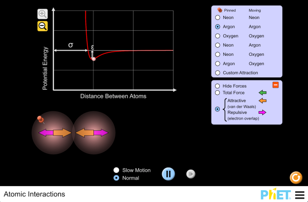
Figure 12.6:The potential energy curve between two atoms, with the atom types adjustable. The equilibrium separation, the well depth, and the curvature at the minimum are the bond length, the bond energy, and the vibrational spring constant respectively.
Interactive simulation: Atomic Interactions
Independently, the molecule can rotate about its center of mass; treating the two nuclei as point masses at fixed separation (the rigid rotor approximation, reasonable when rotational energies are small compared to vibrational spacing) makes this exactly the angular-momentum problem of Chapter 9, with quantized rotational energy
where is the molecule’s moment of inertia and plays the role of the orbital angular momentum quantum number . Because for a typical molecule is large (bond lengths of order , but heavy nuclear masses) compared to the effective “moment of inertia” scale set by an electron, rotational energy spacings are much smaller than vibrational spacings, which are in turn much smaller than electronic transition energies — a hierarchy () that is directly reflected in molecular spectra: electronic transitions lie in the visible/ultraviolet, vibrational transitions in the infrared, and pure rotational transitions in the microwave region, each region probing a different aspect of molecular structure.
This hierarchy is not merely a table of numbers; it is why a molecule responds to one part of the spectrum and ignores another, and Figure 12.7 lets it be tested one photon at a time. Aim microwaves at a molecule and it rotates. Switch to infrared and it starts to vibrate — but only if the vibration changes the molecule’s dipole moment, which is why and have no strong fundamental electric-dipole absorption in the infrared while and do, and hence why the two minor constituents of the atmosphere, not the two major ones, set the temperature of the planet. At sufficiently short ultraviolet wavelengths, a photon can excite an electronic state and may have enough energy to dissociate the molecule.
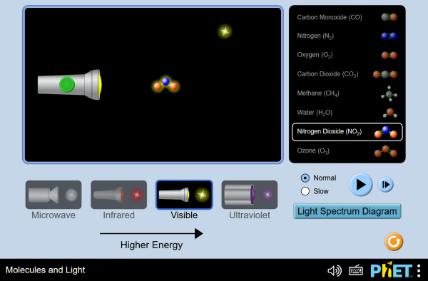
Figure 12.7:Single photons of a chosen wavelength directed at a chosen molecule. Microwave, infrared, visible, and ultraviolet photons each produce a different response — rotation, vibration, electronic excitation, or dissociation — in the order of the hierarchy.
Interactive simulation: Molecules and Light
The Rovibrational Spectrum: Vibration and Rotation Together
A real infrared absorption spectrum does not show the vibrational transition as a single line at . Because a molecule is simultaneously vibrating and rotating, a photon absorbed in a vibrational transition () is generally accompanied by a simultaneous change in rotational state, subject to the selection rule
(for a diatomic molecule, whose single vibrational mode necessarily oscillates the dipole moment along the bond axis itself, quantum-mechanical selection rules for this type of vibration forbid — the analog of a missing branch — leaving only available; some polyatomic vibrations that shift the dipole moment perpendicular to a molecular symmetry axis do permit a weak branch, but a diatomic never has that option). Writing the combined vibration–rotation energy as , with the rotational constant (an energy, in the convention used throughout this chapter), the photon energy absorbed in a transition from to is
Two families of lines result, sketched in Figure 12.8. The R branch (, ) works out to for , giving lines above spaced by . The P branch (, ) works out to for , giving lines below , also spaced by . No line appears at itself — that would be the forbidden Q branch — leaving a characteristic gap of about at the center of the band, a gap that is itself a direct, measurable signature of the selection rule.
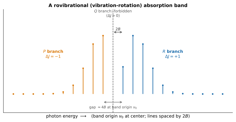
Figure 12.8:A rovibrational absorption band. The branch () and branch () each consist of lines spaced by ; the missing branch (, forbidden for a diatomic) leaves a gap of about at the band origin. Line intensities (schematic here) track the thermal population of each rotational level before absorption.
Because depends only on the molecule’s moment of inertia, measuring the line spacing in a single rovibrational (infrared) spectrum determines — and hence the bond length — directly, without needing a separate microwave (pure-rotation) measurement at all.
Worked Example: Line Spacing in the CO Rovibrational Spectrum
Using the same carbon monoxide data as Problem 5 (, ), find the rotational constant and the resulting rovibrational line spacing.
The moment of inertia is
so
Both branches are spaced by — the same energy as the pure rotational transition of Problem 5, as it must be, since both quantities are just measured two different ways. Converting to the wavenumber units () conventional in infrared spectroscopy,
so the predicted line spacing is — in excellent agreement with the spacing of about actually observed in the CO fundamental infrared band. A bond length and a reduced mass, fed into a formula derived from nothing more than the rigid-rotor approximation, correctly predict the fine structure of a real molecular spectrum.
Anharmonicity Revisited
Figure 12.6, above, already showed that the true interatomic potential is not a perfect parabola: it rises more steeply than quadratic at short range (the repulsive wall) and flattens out well below quadratic at long range, approaching the dissociation energy asymptotically rather than climbing forever. A more realistic potential — the Morse potential is the standard choice for modeling this curve quantitatively — gives vibrational energy levels that are no longer exactly evenly spaced:
where the small, positive anharmonicity constant (typically a few percent, for real molecules) quantifies the departure from a perfect harmonic oscillator. The negative correction term grows with , so the levels crowd closer together at higher — an effect invisible near the bottom of the well, where the potential is well approximated by the parabola of the harmonic-oscillator treatment above, but increasingly important as climbs toward the dissociation limit, where the level spacing approaches zero as the bound levels approach the molecule’s bond dissociation energy. Anharmonicity also relaxes the strict selection rule of the ideal harmonic oscillator, permitting weak overtone transitions with — additional, much fainter absorption lines at roughly (but not exactly) integer multiples of the fundamental frequency. This is why a real vibrational spectrum shows one strong fundamental band accompanied by a series of progressively weaker overtones, rather than the single, perfectly sharp line the ideal harmonic oscillator of Chapter 8 would predict.
12.4Summary
Chemical bonds lower a molecule’s total energy relative to separated atoms; ionic bonding (electron transfer, electrostatic attraction) and covalent bonding (shared electron pairs, enhanced internuclear electron density) are limiting cases of a continuum set by electronegativity difference.
Valence bond theory builds bonds from overlapping atomic orbitals ( for direct, for sideways overlap); hybrid orbitals (, , , etc.), one set per number of electron domains, reproduce observed molecular geometries via minimization of electron-pair repulsion.
Molecular orbital theory builds orbitals belonging to the whole molecule as linear combinations of atomic orbitals, splitting into lower-energy bonding and higher-energy antibonding orbitals; filling these with the molecule’s electrons gives the bond order, which predicts stability, bond strength, and (via unpaired electrons) paramagnetism — correctly predicting, e.g., ’s paramagnetism and the absence of a conventional covalent bond in .
A bonded diatomic molecule has quantized vibrational levels, (harmonic oscillator in the reduced mass ), and rotational levels, (rigid rotor), with , placing electronic, vibrational, and rotational spectra in the UV/visible, infrared, and microwave regions respectively.
The ordering inverts between light second-row diatomics (–, lower via strong – mixing) and heavier ones (–, lower); higher bond order predicts a shorter, stronger bond, confirmed across N–N single/double/triple bonds and by ionizing , , and .
Intermolecular forces — London dispersion (universal, grows with polarizability), dipole–dipole (permanent dipoles), and hydrogen bonding (an unusually strong dipole–dipole interaction specific to H bonded to N, O, or F) — act between already-bonded molecules and set melting and boiling points; comparing molecules of similar size isolates each contribution.
A rovibrational spectrum combines a vibrational transition with a simultaneous rotational one, producing -branch () and -branch () lines spaced by , with a missing central branch (, forbidden for a diatomic); anharmonicity of the real interatomic potential crowds vibrational levels together at high and permits weak overtone transitions.
12.5Problems
Solution to Exercise 12.1 #
VSEPR counts electron domains. Ammonia has four domains, so nitrogen is hybridized; one lone pair makes its molecular geometry trigonal pyramidal. Carbon dioxide has two domains, so carbon is hybridized and the molecule is linear. Sulfur hexafluoride has six domains, so sulfur is hybridized with octahedral geometry.
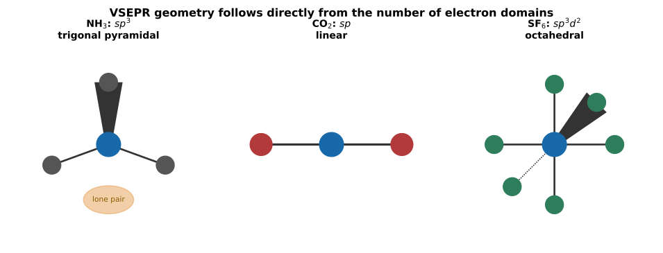
Figure 12.9:Electron-domain count alone fixes the shape: four domains (one a lone pair) bends into a pyramid, two domains keep straight, and six domains spread ’s bonds into an octahedron.
Therefore, the predicted geometries are trigonal pyramidal for , linear for , and octahedral for .
Solution to Exercise 12.2 #
Being isoelectronic with , the ten valence electrons of fill the same sequence of orbitals in the same order:
There are 8 bonding and 2 antibonding electrons, so
Therefore, MO theory predicts bond order 3 for , agreeing with the triple bond in the Lewis structure — the same result found for in Figure 12.5, as expected for two isoelectronic molecules.
Solution to Exercise 12.3 #
For , two electrons occupy bonding and one occupies antibonding . Thus
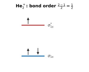
Figure 12.10:Two bonding electrons and one antibonding electron leave a net half a bond — weaker than ’s full bond, but not zero like neutral .
Therefore, is predicted to have a weak, marginally stable half-order bond.
Solution to Exercise 12.4 #
Solution to Exercise 12.5 #
Solution to Exercise 12.6 #
The highest occupied orbitals of are antibonding orbitals. Adding an electron to make raises the antibonding count and lowers bond order by ; removing one to make lowers the antibonding count and raises bond order by — the same level marked in Figure 12.5's diagram is where both changes happen. Therefore, superoxide has a weaker, longer bond, whereas dioxygenyl has a stronger, shorter bond.
Solution to Exercise 12.7 #
has five electron domains, so sulfur uses hybridization and has trigonal-bipyramidal electron-domain geometry. A lone pair preferentially occupies an equatorial site, where it has only two interactions rather than three. The four atoms then form a seesaw geometry.
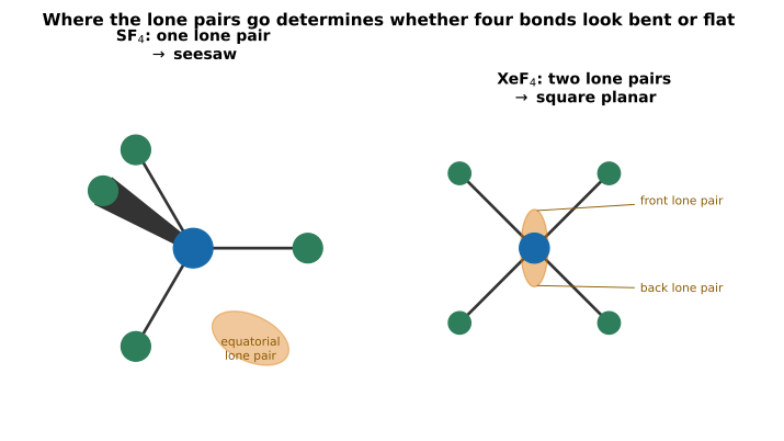
Figure 12.11:One equatorial lone pair pushes ’s four bonds into a lopsided seesaw; a second lone pair, forced to the opposite axial position, symmetrizes the remaining four bonds into a flat square.
Therefore, one equatorial lone pair gives a seesaw shape, whereas two lone pairs in occupy both axial-equivalent arrangements that leave a square planar molecular shape.
Solution to Exercise 12.8 #
The fourteen valence electrons fill
Thus and , giving bond order . Ionization removes an electron from the highest, antibonding level, so has bond order 1.5. One unpaired electron remains in .
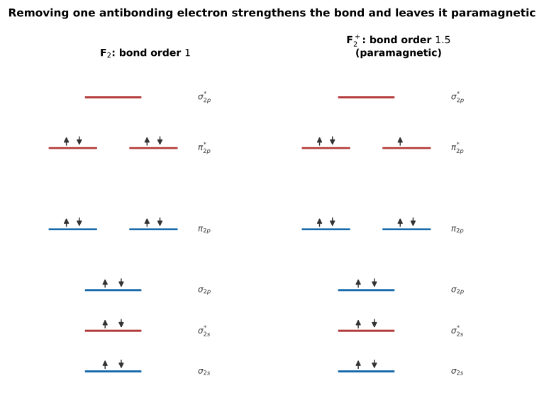
Figure 12.12:Removing one electron from an antibonding level does double duty: it raises the bond order from 1 to 1.5 and leaves one electron unpaired, making paramagnetic where neutral is not.
Therefore, neutral has a single bond, while is paramagnetic and has a stronger, shorter bond.
Solution to Exercise 12.9 #
Using from Problem 4 and ,
The wavenumber , so adjacent rovibrational lines are apart. The missing branch leaves a central gap of between the nearest and lines — the same structure Figure 12.8 draws in general, with HCl’s own numbers filled in. Therefore, HCl has the stated moment of inertia, , line spacing, and a central gap.
Solution to Exercise 12.10 #
All four halogens are nonpolar, so their rising boiling points are not caused by permanent dipoles. Down the group, the electron cloud contains more electrons and is larger and more easily distorted; its polarizability increases. Stronger instantaneous induced dipoles then give stronger London dispersion forces and require more thermal energy to separate molecules. Therefore, the rising boiling points are caused chiefly by increasing molecular polarizability (and associated electron-cloud size).