Learning Objectives
By the end of this chapter, you should be able to:
State the Pauli exclusion principle and explain its role in determining atomic structure.
Explain why the energy of a state in a multi-electron atom depends on both and , unlike in hydrogen, using the concept of electron screening.
Write the ground-state electron configuration of a given element using the subshell-filling order and Hund’s rule.
Relate the structure of the periodic table (periods, groups, blocks) to electron configurations.
Explain the origin of characteristic X-ray spectra and apply Moseley’s law.
Describe the physical basis of the laser: stimulated emission, population inversion, and metastable states.
Introduction
Chapter 10 solved the hydrogen atom exactly, obtaining energies that depend on a single quantum number and states that can be filled with electrons two at a time (spin up, spin down) up to a degeneracy of . This chapter asks what happens for atoms with more than one electron, where the Schrödinger equation cannot be solved exactly, because each electron interacts not only with the nucleus but with every other electron. Two ideas make the many-electron problem tractable and explain the entire structure of the periodic table: an independent-particle approximation, in which each electron is imagined to move in an effective, average potential created by the nucleus and all the other electrons, and the Pauli exclusion principle, a rule with no classical analog that limits how many electrons can occupy any single quantum state. Together they explain why elements have the chemical and spectroscopic properties they do — and, in doing so, resolve one of the oldest puzzles in physics that quantum mechanics was built to explain: the periodic table itself.
11.1The Exclusion Principle and Screening
The Pauli Exclusion Principle
Wolfgang Pauli proposed in 1925 (before the discovery of the Schrödinger equation) a rule required to explain observed atomic spectra and, later, understood as a consequence of the fundamentally indistinguishable and antisymmetric nature of electron wave functions: no two electrons in an atom can occupy the same complete set of quantum numbers . Equivalently, each distinct spatial-and-spin quantum state can hold at most one electron. This is not a subtle statistical tendency but an absolute prohibition, and it applies generally to electrons (and more broadly to the class of particles called fermions, which includes protons and neutrons) — without it, every electron in a multi-electron atom could simply fall into the lowest-energy state, and all atoms would have similar, small sizes and similar chemistry, in sharp contradiction to the observed diversity of the periodic table. The exclusion principle is the single most important input, beyond the Schrödinger equation itself, needed to explain atomic structure.
Historical Context: Pauli’s Reasoning and Hund’s Empirical Rule
Pauli arrived at the exclusion principle in late 1924 by a route that had nothing to do with wave mechanics, which did not yet exist — Schrödinger’s equation was still two years away. Working instead from the older Bohr–Sommerfeld quantum theory, Pauli was trying to explain two stubborn regularities that orbital quantum numbers alone could not account for: the precise electron counts (2, 8, 8, 18, ) at which successive shells close to give a noble gas, and the “anomalous” Zeeman splitting of certain spectral lines into a number of components inconsistent with any known combination of and . Pauli proposed that the electron carries an additional, two-valued property — which he described, before its physical meaning as spin was proposed by Goudsmit and Uhlenbeck the following year, only as a “classically non-describable two-valuedness” — and that no two electrons in an atom may share an identical set of all their quantum numbers, orbital and this new one included. Both puzzles fell into place at once: the shell-closing numbers became simple counting exercises, and the anomalous splittings became ordinary Zeeman splittings of a spin degree of freedom nobody had previously included.
Hund’s rule has a similarly empirical origin. Friedrich Hund formulated it around 1925 not from any first-principles calculation but by systematically cataloging the term symbols (the quantum numbers characterizing the total orbital and spin angular momentum) that best fit the observed ground-state spectra of many atoms, and noticing that the ground state was consistently the one with maximum total spin. Only later, once the Schrödinger equation and the antisymmetry of many-electron wave functions were understood, did it become clear why: electrons with parallel spins are already kept apart by the exclusion principle itself (their spatial wave function must be antisymmetric, vanishing whenever two such electrons approach the same point), which lowers their mutual Coulomb repulsion energy compared to electrons of opposite spin occupying the same orbital. This spin-correlated reduction in repulsion is called the exchange energy, and it reappears below as the reason certain elements (chromium and copper among them) deviate from the naive Aufbau filling order.
The Real Content of the Exclusion Principle: Antisymmetric Wave Functions
Stated as “no two electrons can share the same quantum numbers,” the exclusion principle can look like an arbitrary bookkeeping rule bolted onto quantum mechanics. Its actual origin is a deeper and more general statement about identical particles: because electrons are fundamentally indistinguishable, swapping the labels of any two electrons in a multi-electron wave function must leave every measurable prediction unchanged, which requires the total wave function to be either symmetric or antisymmetric under that exchange. Experiment (and the spin-statistics theorem) fixes electrons, as spin- fermions, to the antisymmetric choice.
For two electrons in single-particle states and , the properly antisymmetrized two-electron wave function is
Swapping the labels multiplies by -1, as required of a fermion wave function. Now suppose the two states are the same, : the expression becomes identically. The wave function for two electrons in the same quantum state does not merely describe an unlikely configuration — it vanishes outright, for every possible position and spin of both electrons. “No two electrons occupy the same state” is not a separate postulate; it is this algebraic fact, stated in words. The same antisymmetry, applied to two electrons in different orbitals with parallel spin, is also what produces the exchange energy discussed above: the antisymmetric spatial wave function is forced toward zero whenever the two electrons approach the same point, keeping same-spin electrons farther apart on average and lowering their mutual Coulomb repulsion.
Screening and Subshell Energies
In hydrogen, the energy of a state depends only on (Chapter 10), because the electron feels the bare potential of a single proton. In a multi-electron atom, an electron in an outer shell is partially screened from the full nuclear charge by the electrons in shells closer to the nucleus: it feels an effective nuclear charge , reduced from the true charge by the (partial) shielding effect of the intervening electron cloud.
Screening depends on as well as , because electrons of lower (at fixed ) have wave functions with a greater probability of being found close to the nucleus (their radial probability distributions extend closer to , as can be seen in the general shape of the hydrogen radial functions of Chapter 10) — such electrons penetrate the inner electron cloud more effectively, feel less screening, and are therefore more tightly bound. The result is that, unlike in hydrogen, energy in a multi-electron atom depends on both and , with energy generally increasing with at fixed : within a given , an state () lies lower in energy than a state (), which lies lower than a state (), and so on. This -dependence is what breaks hydrogen’s accidental degeneracy and is responsible for the specific subshell-filling order used below.
The Self-Consistent Field: How Screening Is Actually Computed
The qualitative picture above — “an electron feels a reduced effective charge ” — can be made into an actual calculation, and doing so is instructive even though the resulting numbers are only ever approximate. Douglas Hartree, in 1928, proposed treating each electron as moving independently in an effective, spherically averaged potential built from the nucleus plus the smeared-out charge distribution of every other electron: . The trouble is circular — computing requires already knowing the wave functions of all the other electrons, which is exactly what one is trying to find. Hartree’s resolution, the self-consistent field (SCF) method, is an iterative procedure: start with a reasonable guess for every electron’s wave function (hydrogen-like orbitals, say); use those guesses to compute an averaged charge density and hence an effective potential for each electron; solve the resulting one-electron Schrödinger equation for each electron in that potential, obtaining improved wave functions; recompute the charge density and the effective potential from these improved wave functions; and repeat. The cycle is stopped once the potential fed in and the potential computed out agree to the desired precision — the field is then “self-consistent,” and the resulting energies and wave functions are the Hartree approximation’s best estimate for the atom’s structure. (A refinement due to Vladimir Fock in 1930, Hartree–Fock theory, additionally enforces the antisymmetry required by the exclusion principle itself, which plain Hartree theory omits, and is the starting point for essentially all modern atomic-structure and quantum-chemistry calculations.)
This procedure makes the -dependence of screening explicit rather than assumed: an electron that penetrates inside the charge cloud of the other electrons (small ) sees a potential close to the full, unscreened nuclear charge , while an electron that stays outside essentially all the other electrons (large ) sees a much-reduced net charge — roughly minus the number of electrons enclosed within its orbit. A full SCF calculation is impractical by hand, which is why Slater’s rules (1930) exist: an empirical, hand-computable recipe, calibrated against Hartree-type results, for estimating a single number for a given electron without running the iteration at all.
Worked Example: Effective Nuclear Charge via Slater’s Rules
Slater’s rules group orbitals as , , , , , and estimate the total screening felt by an electron in an or orbital as a sum of contributions: 0.35 for each other electron in the same group (0.30 if the group is ), 0.85 for each electron one shell lower (), and 1.00 (full screening) for each electron two or more shells lower. Then .
For the single valence electron of sodium (, configuration ), the electron of interest is the lone electron. There are no other electrons in its group; the shell contributes 8 electrons () at 0.85 each; the shell contributes 2 electrons at 1.00 each:
For a electron of chlorine (, configuration ), the same-group electrons are the remaining 6 electrons of (excluding the one of interest), the shell again contributes 8 electrons at 0.85, and the shell contributes 2 at 1.00:
Moving across period 3 from sodium to chlorine, the true nuclear charge grows by 6 protons, but the added electrons (all in the same shell) screen each other only weakly (0.35 each rather than 0.85 or 1.00), so very nearly keeps pace with , rising from 2.20 to 6.10 — nearly a threefold increase. This is the quantitative content behind the qualitative statement that effective nuclear charge rises sharply across a period, and it is the mechanism explored further below in connection with ionization energy and atomic size.
11.2Electron Configurations and the Periodic Table
Combining the exclusion principle with the ,-dependent ordering of subshell energies, the ground-state electron configuration of an atom is built by filling the lowest-energy available subshells first, two electrons (spin up and spin down) per orbital, up to electrons per subshell — this is the Aufbau (“building-up”) principle. Because screening shifts subshell energies, the filling order does not simply follow increasing ; the empirical (and largely first-principles-derivable) order is approximately
— note, for example, that fills before , since the extra penetration of the orbital lowers its energy below that of despite its larger . When a subshell contains more than one electron and is only partially filled, Hund’s rule states that the ground-state configuration maximizes the total spin (electrons singly occupy separate orbitals within a subshell, with parallel spins, before any orbital is doubly occupied) — a consequence of electron-electron repulsion, which is minimized when electrons, to the extent the exclusion principle allows, avoid occupying the same spatial orbital.
This filling scheme directly generates the structure of the periodic table. Each period (row) begins filling a new principal shell ; in the transition and inner-transition blocks, however, a lower- or subshell is filled after the outer subshell, so a period is not simply a single-shell filling sequence. Each period ends when every subshell filled so far is completely full, the particularly stable arrangement that defines a noble gas. Elements in the same group (column) generally share the same outer-shell (valence) configuration and, correspondingly, similar chemical properties, since chemical bonding (Chapter 12) is governed primarily by the valence electrons. The table’s division into -block, -block, -block (transition metals), and -block (lanthanides/actinides) regions directly reflects which subshell is being filled across that block. The chemical inertness of the noble gases, the strong reactivity of the alkali metals (a single, loosely bound -electron outside a filled shell) and the halogens (one electron short of a filled shell), and the broad periodicity of atomic size and ionization energy all follow from this shell structure, without further assumptions.
The Aufbau procedure is quicker to learn by doing it than by reading the rules, and Figure 11.1 is the exercise: add protons, neutrons, and electrons one at a time and watch the element name, the net charge, the mass number, and the shell occupancy update together. Two habits of thought are worth breaking there. Adding a proton changes the element; adding a neutron does not, and only moves the atom along a row of isotopes (Chapter 13). And the electrons go into shells that fill in a fixed order, so that the chemistry of the atom is decided by the last few added rather than by the total.
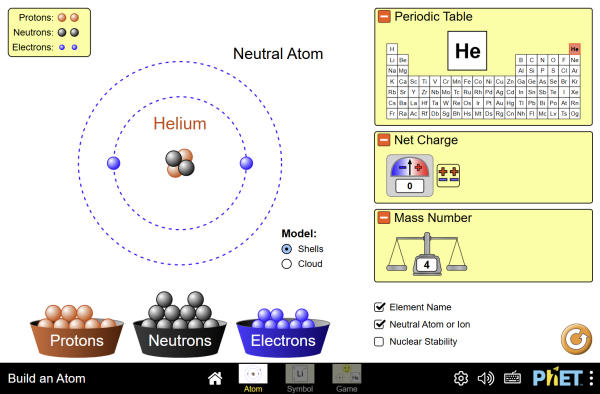
Figure 11.1:Atoms assembled particle by particle, with element, charge, mass number, and electron shell filling all displayed as they are built. Build up to neon or argon and the outer shell closes exactly as the electron count reaches a noble gas — the closure being a fact about the electrons, and nothing to do with the nucleus underneath them.
Interactive simulation: Build an Atom
The Aufbau Order in Practice: Configurations Across the Periodic Table
The filling order is best seen applied across a representative spread of the periodic table, rather than for one or two elements in isolation. Table 11.1 builds ground-state configurations by strict Aufbau filling for most entries, but flags two elements — chromium and copper — where the real, spectroscopically measured ground state disagrees with the naive prediction, and includes lanthanum, the first element for which the subshell becomes energetically relevant, as a further illustration of just how close some subshell energies run to one another.
Table 11.1:Ground-state electron configurations across the periodic table, by strict Aufbau filling order.
| Element | Naive Aufbau prediction | Actual ground state | |
|---|---|---|---|
| Helium | 2 | ||
| Neon | 10 | ||
| Argon | 18 | ||
| Potassium | 19 | ||
| Calcium | 20 | ||
| Scandium | 21 | ||
| Chromium | 24 | (exception) | |
| Iron | 26 | ||
| Copper | 29 | (exception) | |
| Krypton | 36 | ||
| Lanthanum | 57 | (exception) |
Two features stand out. First, every noble gas (, , , ) ends a row with every subshell up to that point completely filled — the defining structural feature of a noble gas, and the reason the next electron (starting a new period) must go into a new, much less tightly bound shell, exactly the drop in binding responsible for the alkali metals’ low ionization energy discussed below. Second, three of the eleven entries in the table are Aufbau exceptions, which is a useful reminder that the filling order given earlier in this chapter is a good approximation, not an exact law — the true ordering is whatever a full self-consistent-field calculation (or, in practice, the measured spectrum) says it is, and the mnemonic order is simply the pattern that calculation follows most of the time.
Worked Example: Why Chromium’s Ground State Breaks the Naive Aufbau Order
The Aufbau order predicts chromium () should have configuration : fill completely (it is lower in energy than , as established above), then place the remaining four electrons in . The measured ground state is instead — one electron has been promoted from down into , apparently uphill in single-particle energy.
The resolution is that single-particle subshell energies are not the whole story; the total energy of the atom also includes the electron-electron interaction energy, and that interaction is lower, for a fixed set of occupied orbitals, when as many electrons as possible have parallel spin (the exchange energy discussed in the Historical Context box above). The configuration places one electron in each of the five orbitals () with parallel spin, and the electron can align with them as well. In the naive configuration, only four orbitals are singly occupied, while the orbital is paired and the fifth orbital is empty. The half-filled subshell therefore gains substantial exchange stabilization, and for chromium specifically that extra lowering outweighs the modest single-particle energy cost of moving one electron from up into . Copper () is analogous: trades a doubly occupied for a completely filled, maximally stable shell (all orbitals doubly occupied — no further exchange gain from that shell alone, but a filled subshell carries its own extra stability, being spherically symmetric and having zero net orbital angular momentum) rather than the naive . These familiar exceptions occur at half-filled () and completely filled () subshells, where exchange and subshell-closure effects can favor the promotion.
Ionization Energy and Atomic Radius Across the Periodic Table
The Slater’s-rule calculation above — rising from 2.20 (sodium) to 6.10 (chlorine) across period 3 — is the quantitative content behind two of the most familiar patterns in chemistry. Atomic radius decreases across a period: each added electron goes into the same shell (same , hence similar average distance from the nucleus, all else equal), while pulling on that shell steadily increases, drawing the whole electron cloud inward. First ionization energy — the energy required to remove the least tightly bound electron — correspondingly increases across a period, since a more tightly bound (higher , smaller-radius) electron is harder to remove; sodium’s outermost electron () is far easier to strip away than chlorine’s (), consistent with the roughly threefold increase in found above. Both trends reverse on descending a group: each new period adds a shell of larger , and although for the outermost electron changes only mildly down a group (the added inner shells screen the added protons quite effectively, shell for shell), the larger dominates, so atomic radius grows and ionization energy falls — lithium, sodium, and potassium have successively lower first ionization energies (5.39, 5.14, ) even though more than sextuples between them.
Figure 11.2 shows the resulting pattern for every element from hydrogen through krypton: not a smooth trend but a sharp periodic sawtooth, rising across each period and collapsing at the start of the next, with a noble gas at every peak and an alkali metal at every trough — the periodic table’s defining periodicity made directly visible in a single measurable quantity.
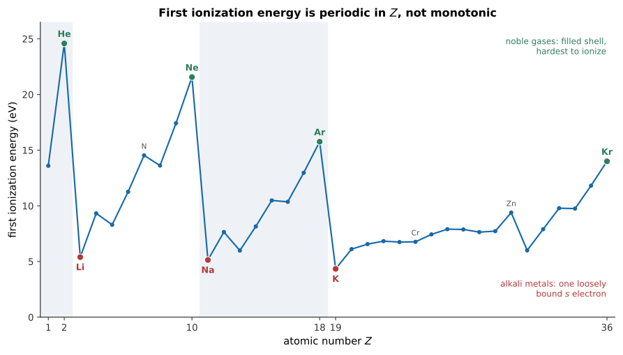
Figure 11.2:First ionization energy versus atomic number, –36. Each period rises from an alkali-metal trough to a noble-gas peak as grows across the period, then collapses as a new, more distant shell begins. Computed from NIST Atomic Spectra Database ionization-energy values.
Two smaller features in that figure repay a closer look. Within period 2, beryllium’s ionization energy () is higher than boron’s (), even though boron has one more proton — a small step backward against the overall rising trend, and the same pattern recurs for nitrogen () against oxygen (), and again in period 3 for phosphorus () against sulfur (). These dips are not noise; they are the same subshell-stability physics responsible for the chromium and copper exceptions above, showing up in ionization energy instead of in the filling order.
Worked Example: The Ionization-Energy Dips at Boron and Oxygen
Beryllium’s configuration is . Removing an electron from boron (), by contrast, means removing the single electron — a higher-energy, more weakly bound (less penetrating, more screened) subshell than — which is easier despite boron’s larger nuclear charge. The key is the subshell ordering produced by penetration and screening: the added boron electron enters a subshell that lies above , rather than a general rule that every filled subshell is unusually stable. There is also no exchange-energy advantage for boron’s lone electron comparable to the half-filled case discussed next.
Nitrogen’s configuration is : a half-filled subshell, with all three electrons in separate orbitals with parallel spin, by Hund’s rule. Oxygen () must place its fourth electron into an orbital that already holds one — pairing two electrons in the same spatial orbital, with opposite spins, for the first time in the subshell. That pairing adds direct Coulomb repulsion between the two electrons sharing an orbital and removes some of the exchange stabilization associated with the half-filled arrangement. Both effects make oxygen’s paired electron easier to remove than any of nitrogen’s three unpaired ones, despite oxygen’s larger nuclear charge — exactly the same underlying mechanism (exchange-energy stabilization of half-filled subshells) that pins chromium at rather than .
11.3Atomic Spectra, X-Rays, and Lasers
Atomic Spectra and X-Rays
Optical spectra of multi-electron atoms arise, as in hydrogen, from transitions of a single (typically outer, valence) electron between energy levels, now shifted by screening as described above and further split by the interaction between an electron’s orbital and spin magnetic moments (spin-orbit coupling), producing the closely spaced doublets and multiplets seen in high-resolution atomic spectra.
A distinct and higher-energy class of spectral lines, characteristic X-rays, arises from transitions of inner-shell electrons. If an atom is bombarded with sufficiently energetic electrons (as in an X-ray tube) or photons, an inner-shell electron (e.g., from the , or , shell) can be ejected entirely, leaving a vacancy. An electron from a higher shell then drops down to fill the vacancy, emitting a photon whose energy — since inner-shell electrons in heavier atoms feel nearly the full, largely unscreened nuclear charge — is far larger than typical optical-transition energies, and falls in the X-ray part of the spectrum. X-ray spectroscopists label shells by letter rather than by : is the shell, the shell, the shell, the shell, and so on — a historical notation, predating the Bohr model, that has simply stuck. Lines from transitions ending on the shell are called the K series (with for the , i.e. , transition, for , i.e. , etc.); an atom with a vacancy in the shell instead produces the analogous, lower-energy series ( for , and so on).
Henry Moseley (1913) measured the characteristic X-ray frequencies of many elements and found that the frequency of the line follows a strikingly simple pattern, Moseley’s law:
where and are constants (with for the line, reflecting screening of the nuclear charge by the one remaining -shell electron) essentially independent of the element. This relation follows directly from a hydrogen-like treatment of the transition, with the true nuclear charge replaced by an effective charge to account for screening by the other -shell electron, applied to the Bohr/Schrödinger hydrogen energy formula. Moseley’s law provided, for the first time, a direct physical (rather than merely chemical) way to determine an element’s atomic number , and was used to correctly order elements in the periodic table, resolve several ambiguities in the ordering by atomic mass, and confirm the existence of predicted-but-then-unobserved elements by their expected X-ray frequency, cementing (nuclear charge) rather than atomic mass as the correct organizing quantity for the periodic table.
The Moseley Plot
Moseley’s own presentation of his data was graphical rather than tabular, and remains the clearest way to see the law’s content: plotting (the square root of the measured frequency) against for every element measured produces, to remarkable precision, a single straight line. That linearity is the entire empirical claim — a hydrogen-like energy spectrum predicts , i.e., , so a plot linear in is direct evidence that inner-shell transition energies really do scale as a screened hydrogen atom’s, even in atoms far too complicated to solve exactly. The same linear relationship holds separately for the series and other series, each with its own slope and intercept (the -series screening constant is larger than the -series value of about 1, since an -shell vacancy is screened by more surrounding electrons than a -shell vacancy is) — a family of parallel diagnostic lines, one per series, any one of which pins down from a measured frequency alone.
Worked Example: Moseley’s Law — Predicting Nickel’s Line from Copper’s
A single measured frequency, together with the known screening constant , is enough to predict the frequency of a neighboring element. Copper () has a measured frequency (corresponding to a photon energy , close to the accepted value of for the Cu line). Writing Moseley’s law as and solving for using copper’s data,
Applying the same to nickel (, one proton lighter),
corresponding to a predicted photon energy . The accepted experimental value for the Ni doublet is 7.461– — agreement to better than half a percent, from a calculation using only a single measured data point and one universal constant, exactly the kind of predictive power that let Moseley assign atomic numbers to elements from X-ray measurements alone.
The surviving photograph in Figure 11.3 shows the physicist himself, not long before the work described above.
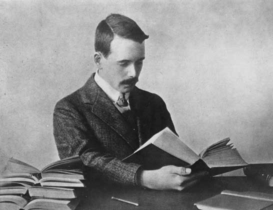
Figure 11.3:Henry Gwyn Jeffreys Moseley, circa 1914. Photograph via the AIP Emilio Segrè Visual Archives, W. F. Meggers Gallery of Nobel Laureates; public domain via Wikimedia Commons.
Historical Context: Henry Moseley and the 1913–1914 X-Ray Survey
Henry Moseley was 26 years old, working at Ernest Rutherford’s laboratory in Manchester and then at Oxford, when he built an X-ray spectrometer and, over roughly a year, measured the characteristic - and -series frequencies of nearly 40 elements — an extraordinarily fast and thorough experimental survey by the standards of the day. The result was immediately and directly useful to chemistry: several elements were known, from their chemical properties, to sit in a different order than their measured atomic masses would suggest (tellurium and iodine are the classic example — tellurium is heavier but chemically belongs before iodine in the periodic table), and Moseley’s X-ray frequencies confirmed that atomic number, not mass, was the correct ordering quantity in every such case. His data also revealed gaps: no element then known produced the frequency predicted for , 61, or 75, and Moseley correctly concluded that these elements simply had not yet been discovered (they are now known as technetium, promethium, and rhenium; technetium and promethium are highly radioactive and occur only in trace amounts naturally. Technetium was identified in 1937 after being produced from a cyclotron target, although trace natural technetium does exist). A vacancy at was, for a decade, the subject of a bitter chemical priority dispute — a French chemist had already claimed the element among the rare earths and named it “celtium” — until 1922, when X-ray measurements at Bohr’s institute in Copenhagen showed conclusively that the true element 72 (hafnium) is chemically a heavier relative of zirconium, not a rare earth at all, and had simply been misidentified.
Moseley enlisted in the Royal Engineers at the outbreak of the First World War and was killed at Gallipoli on 10 August 1915, at 27, shot through the head while relaying a message during the landing. His death is often cited (including by later Nobel laureates who worked to change the practice) as a direct argument for the British and other governments’ subsequent policy of not sending scientifically valuable personnel to serve at the front line — a policy adopted too late to save Moseley himself, whose X-ray survey had already, in barely two years, put the periodic table’s underlying organizing principle beyond doubt.
At the optical end of the same physics, Figure 11.4 runs the experiment a neon sign runs: electrons accelerated through a low-pressure gas, colliding with atoms, and the light that comes out. The collisions are the point. Below the threshold for inelastic excitation, collisions are mostly elastic and the tube stays dark; raise the accelerating voltage past the first excitation energy and electrons can transfer that discrete excitation energy to the atoms, retaining the rest of their kinetic energy. The excited atoms subsequently emit photons at wavelengths fixed by their allowed transitions, sometimes through cascades of intermediate states. That threshold behavior is the Franck–Hertz experiment, and it is direct evidence of discrete atomic levels that owes nothing to spectroscopy. Multi-level atoms can be selected to see cascades through intermediate states, which is the same level structure the next section exploits.
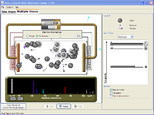
Figure 11.4:A gas discharge tube with the accelerating voltage, the gas, and the atomic energy-level scheme under control. Excitation happens only at discrete electron energies, and the emitted spectrum is the level diagram read out in light.
Interactive simulation: Neon Lights & Other Discharge Lamps
Lasers
A further application of atomic energy levels involves the interaction between atoms and light more actively than simple absorption/emission spectroscopy. An atom in an excited state can lose energy in two distinct ways: spontaneous emission, in which it decays at a random time with a photon emitted in a random direction (governing ordinary fluorescence and, statistically, the exponential decay laws seen throughout atomic and nuclear physics), and stimulated emission, in which a passing photon of exactly the transition energy triggers the atom to emit a second, additional photon that is an exact copy of the first — same energy, direction, phase, and polarization. Einstein first predicted stimulated emission in 1917, well before it could be technologically exploited.
Ordinarily, stimulated emission is masked by the competing process of absorption, since a typical collection of atoms in thermal equilibrium has more atoms in lower-energy states than higher ones. A laser (light amplification by stimulated emission of radiation) requires engineering a population inversion — an atomic sample with more atoms in a higher-energy state than a lower one, typically achieved by “pumping” atoms into a higher state and relying on an intermediate metastable state (one with an anomalously long lifetime against spontaneous decay, because its decay to lower states is forbidden or strongly suppressed by selection rules such as the rule of Chapter 10) to accumulate a population large enough to exceed that of the lower lasing level. Once inverted, a single spontaneously emitted photon can trigger a cascade of stimulated emission as it passes back and forth through the gain medium (typically between two mirrors forming an optical cavity), producing an intense, coherent, highly directional, single-wavelength beam — a direct, large-scale, technological manifestation of discrete atomic energy levels and the quantum-mechanical description of light-matter interaction developed across this and the preceding chapters.
Two Concrete Laser Systems: Helium–Neon and Ruby
The helium–neon (He-Ne) laser, one of the first lasers built (1961) and still common in classrooms and barcode scanners, illustrates a four-level scheme. An electrical discharge through a low-pressure He-Ne gas mixture excites helium atoms into a long-lived metastable state at above the helium ground state — an -state whose direct decay to the (also -state) helium ground level is forbidden by the selection rule, not merely unlikely because of its energy, so helium atoms accumulate there in large numbers, exactly the metastable-state bottleneck described above. That energy happens to very nearly match a neon excited state near , so an excited helium atom colliding with a ground-state neon atom can transfer its energy directly, exciting the neon (and leaving the helium atom free to be re-excited by the discharge) — helium serves purely as an energy-transfer intermediary, never itself the lasing species. The excited neon atom then undergoes stimulated emission down to a lower excited state, emitting the familiar red beam; because that lower level is itself well above the neon ground state and decays away rapidly through further (non-lasing) transitions, it never accumulates a large population, so the population inversion between the upper and lower laser levels is easy to sustain — the defining advantage of a four-level design over a three-level one.
The ruby laser, built by Theodore Maiman in 1960 (the first laser of any kind to operate), is a three-level system and correspondingly harder to pump. Ruby is aluminum oxide doped with a small fraction of chromium ions (), whose electronic transitions (not those of the aluminum oxide host) do the lasing. An intense flash lamp pumps chromium ions from the ground state into two broad, short-lived absorption bands (centered in the blue and green, which is why ruby appears red — it absorbs the complementary colors); those ions decay almost immediately, without emitting a photon, to a metastable level about above the ground state, with a comparatively long lifetime of several milliseconds. Because the lower laser level in this scheme is the atomic ground state itself, which starts out fully populated, achieving a population inversion requires pumping more than half of all the chromium ions into the metastable state simultaneously — a substantially harder threshold to cross than in a four-level scheme, where the lower laser level is nearly empty to begin with. Once inverted, stimulated emission from the metastable level back to the ground state produces ruby’s characteristic deep-red beam, historically in short, intense pulses rather than the continuous output a He-Ne laser can sustain.
Every ingredient of that description is separately adjustable in Figure 11.5, which is the best way to see that a laser is a threshold device rather than a bright lamp. Pump a two-level medium as hard as you like and it will not lase: absorption and stimulated emission from a two-level system saturate at equal populations, so no inversion is possible. Switch to three levels, so that atoms accumulate in a metastable state, and the inversion appears; add the cavity mirrors and, above a pump rate that the simulation makes it easy to bracket from below, the output collapses from a random scatter of spontaneous photons into a single coherent beam.
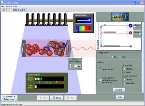
Figure 11.5:A laser assembled from its parts: a pump, a two- or three-level gain medium, and an optical cavity. Population inversion is displayed directly, so the threshold for lasing can be found by experiment rather than asserted.
Interactive simulation: Lasers
Worked Example: Population Inversion Requires Active Pumping
It is worth confirming, numerically, why a population inversion never arises on its own from thermal equilibrium and must be engineered by pumping. In thermal equilibrium at temperature , the ratio of the number of atoms in an upper state (energy ) to a lower state (energy ) is set by the Boltzmann factor,
For the ruby laser transition, (found from with , using ). At room temperature, , , so
Out of every 1030 or so chromium ions in thermal equilibrium, essentially none sit in the upper laser level — an inversion () is not just unlikely but is astronomically, hopelessly far from anything thermal equilibrium could ever produce at ordinary temperature. This is precisely why a laser requires an external pump (an intense flash lamp, an electrical discharge, or another laser) to force the population far out of thermal equilibrium, and why, once the pump is switched off, the inverted population decays and lasing stops — a laser is fundamentally a driven, non-equilibrium device, not a system that has simply been heated.
Applications: Lasers in Technology and Medicine
The properties that make a laser beam distinctive — a single, precisely defined wavelength; a high degree of spatial coherence, allowing the beam to be focused to a tiny spot or to travel long distances with little spreading; and a high degree of temporal coherence, permitting long coherence lengths (Chapter 4) — underlie applications far removed from the gas-discharge tubes and ruby rods described above. Fiber-optic communication, the physical backbone of the modern internet, encodes digital data as pulses from semiconductor diode lasers (a solid-state laser design, distinct from both examples above, in which the population inversion is created electrically across a semiconductor junction rather than by an optical pump) sent down thin glass fibers by total internal reflection; the laser’s narrow wavelength spread keeps different colors of light traveling through the same fiber from smearing into one another over long distances, allowing enormous data rates over transoceanic distances. Laser cooling, by contrast, exploits the momentum carried by individual photons (Chapter 6): a beam tuned just below an atom’s resonant absorption frequency preferentially scatters off atoms moving toward the beam (Doppler-shifted into resonance), each absorption event imparting a momentum kick that opposes the atom’s motion, and repeated scattering from beams in multiple directions can cool a dilute atomic gas to temperatures of a microkelvin or below — a technique essential to modern atomic clocks and to the experimental study of quantum gases. In medicine, lasers are used both destructively, where a tightly focused, high-intensity beam cuts or cauterizes tissue with a precision unavailable to a mechanical scalpel (as in some ophthalmic and dermatological surgery), and diagnostically, where the coherence and narrow linewidth of laser light are exploited in optical coherence tomography to image tissue structure with micrometer resolution — different laser properties from the list above put to work in each case.
11.4Summary
The Pauli exclusion principle forbids two electrons from sharing the same full set of quantum numbers , limiting each orbital to two electrons (opposite spin) and is essential to explaining atomic structure.
Screening of the nuclear charge by inner electrons makes subshell energy depend on both and in multi-electron atoms, unlike hydrogen; lower- orbitals penetrate closer to the nucleus and lie lower in energy at fixed . The self-consistent field (Hartree) method computes screening explicitly, by iterating each electron’s wave function in the averaged potential of all the others until the potential stops changing; Slater’s rules give a fast hand-calculable estimate of the resulting effective nuclear charge .
The Aufbau principle (fill lowest-energy subshells first, respecting exclusion) and Hund’s rule (maximize total spin within a partially filled subshell) determine ground-state electron configurations, which in turn generate the row/column/block structure of the periodic table and the periodicity of chemical properties. Exchange and subshell-closure effects favor especially stable half-filled and completely filled subshells, producing Aufbau exceptions (chromium, copper) and small dips in ionization energy (boron, oxygen) that the naive filling order alone does not predict.
First ionization energy generally rises across a period while atomic radius generally falls, both tracking ; down a group, the trends reverse as increasing dominates a nearly constant .
Characteristic X-rays arise from inner-shell vacancies, labeled by shell letter (: , : , : , ); Moseley’s law, — a straight line when is plotted against — let X-ray spectra be used to determine atomic number directly, correctly ordering the periodic table by and revealing the undiscovered elements , 61, and 75.
Lasers exploit stimulated emission and a population inversion, sustained via a metastable state, to produce coherent light; three-level (ruby) and four-level (helium–neon) schemes differ in how hard the lower laser level is to keep empty. Lasers underlie fiber-optic communication, laser cooling, and a range of medical applications.
11.5Problems
Solution to Exercise 11.1 #
Filling orbitals in the stated energy order gives carbon: ; sodium: ; and iron: . Therefore, these are the respective ground-state electron configurations for , 11, and 26.
Solution to Exercise 11.2 #
Nitrogen has . Hund’s rule puts one parallel-spin electron into each of the three orbitals before any pairing: . The three spins each have , so the total spin quantum number is (and the maximum projection is ).
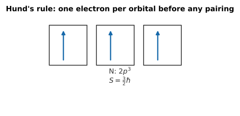
Figure 11.6:Hund’s rule in action: all three orbitals get one electron, spins aligned, before any orbital is filled with a second, opposite-spin electron.
Therefore, nitrogen’s subshell has three unpaired parallel electrons and total spin quantum number (with maximum projection and spin angular-momentum magnitude ).
Solution to Exercise 11.3 #
A electron penetrates toward the nucleus more effectively than a electron, so it spends more time inside the shielding cloud of inner electrons. It consequently feels a larger effective nuclear charge and can have a lower energy despite its larger principal quantum number. Therefore, orbital energy in a many-electron atom depends on penetration and screening, not on alone.
Solution to Exercise 11.4 #
Moseley’s relation with gives . Hence
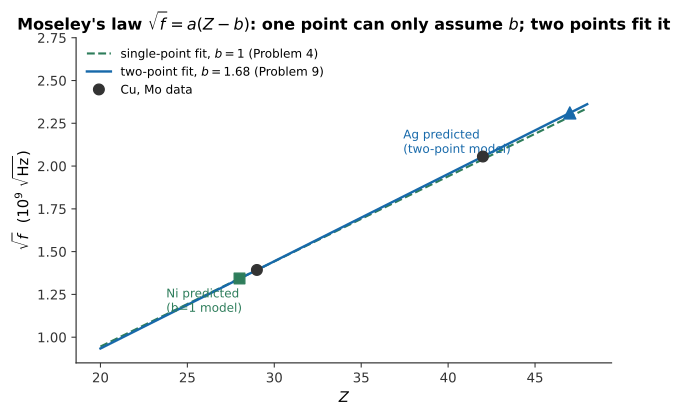
Figure 11.7:This problem’s single-point, extrapolation (dashed) and Problem 9’s two-point fit (solid) nearly coincide over this range — both are straight lines in vs. , just anchored differently.
Therefore, nickel’s predicted frequency is , lower than copper’s because nickel has one fewer proton.
Solution to Exercise 11.5 #
Helium’s orbital is full: the exclusion principle prevents a third electron from entering the same lowest-energy state, so removing or rearranging an electron requires a large energy. Lithium has the closed core plus one weakly bound electron, which can be removed or shared at much lower energy. Therefore, helium is chemically inert while lithium is reactive because lithium has an accessible unpaired outer electron.
Solution to Exercise 11.6 #
Pumping directly to a short-lived allowed-transition level does not build an inversion because that level decays rapidly. A metastable state has a transition to the lower state that is forbidden or strongly suppressed, so its lifetime is long enough for pumped atoms to accumulate above the lasing transition. Therefore, metastability is what permits a sustained population inversion in three- and four-level lasers.
Solution to Exercise 11.7 #
For one magnesium electron, the other electron shields 0.35; the eight electrons shield ; and the two electrons shield . Thus
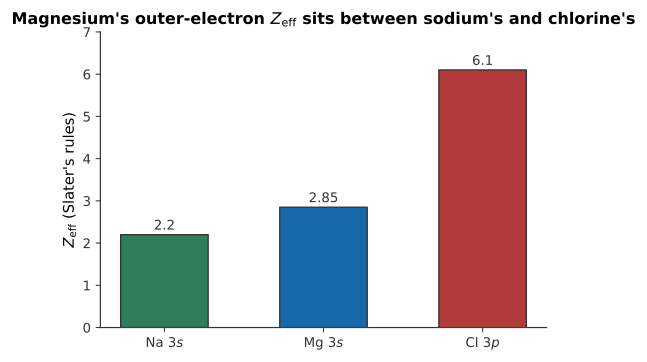
Figure 11.8:Slater’s-rules increases steadily across the period as protons are added faster than shielding can compensate; magnesium’s 2.85 falls exactly between sodium’s and chlorine’s.
Therefore, magnesium’s electron feels , appropriately between sodium’s 2.20 and chlorine’s 6.10.
Solution to Exercise 11.8 #
Phosphorus has , with three parallel electrons in separate orbitals, gaining the stabilization associated with a half-filled subshell. Sulfur is , so one orbital contains a pair; the added electron introduces pairing repulsion and reduces that special exchange stabilization.
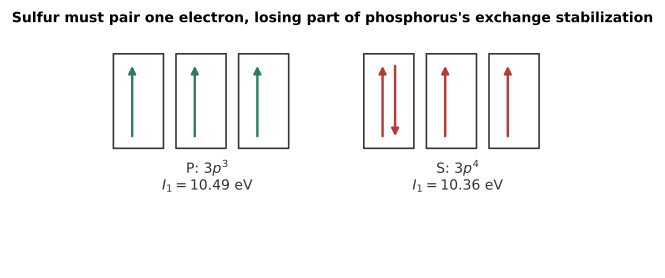
Figure 11.9:Phosphorus keeps every electron unpaired and enjoys the full half-filled-subshell exchange bonus; sulfur’s fourth electron must double up, and the resulting pairing repulsion slightly outweighs its extra proton.
Therefore, sulfur’s first ionization energy is slightly lower than phosphorus’s despite sulfur’s larger nuclear charge.
Solution to Exercise 11.9 #
For molybdenum, . Subtracting for Cu and Mo gives
For silver, , so and , the point extrapolated in Figure 11.7. Therefore, is of order unity and the fitted law predicts a silver photon.
Solution to Exercise 11.10 #
The photon energy is
The photon rate is . Therefore, the laser emits photons at photons/s; its spatial coherence can focus this modest power into a very small retinal spot, making it hazardous.
Solution to Exercise 11.11 #
The electron density determines the screening part of , but that density is obtained only after solving for the electron wave functions in itself. Hartree’s method begins with a trial density, solves the one-electron equations, constructs a new density and potential, and repeats. Therefore, the method is called self-consistent when an iteration returns the same density and effective potential with no material further change.
Solution to Exercise 11.12 #
Across period 3, added protons raise while electrons stay in the shell, so radii generally decrease. Potassium starts a new shell: its electron is farther out and strongly shielded by the filled argon core.
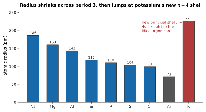
Figure 11.10:Radius falls steadily as grows across a period, then jumps back up the instant a new principal shell opens at potassium.
Therefore, potassium’s new principal shell outweighs its extra proton, giving it a larger radius than argon.